Abstract

We consider a waveguide modeled by the Laplacian in a straight planar strip. The Dirichlet boundary condition is taken on the upper boundary, while on the lower boundary we impose periodically alternating Dirichlet and Neumann condition assuming the period of alternation to be small. We study the case when the homogenization gives the Neumann condition instead of the alternating ones. We establish the uniform resolvent convergence and the estimates for the rate of convergence. It is shown that the rate of the convergence can be improved by employing a special boundary corrector. Other results are the uniform resolvent convergence for the operator on the cell of periodicity obtained by the Floquet-Bloch decomposition, the two-terms asymptotics for the band functions, and the complete asymptotic expansion for the bottom of the spectrum with an exponentially small error term.

1) Bashkir State Pedagogical University, October Revolution St. 3a,
1) 450000 Ufa, Russia, e-mail: borisovdi@yandex.ru
2) LMAM, UMR 7122, Université de Metz et CNRS Ile du Saulcy,
1) F-57045 METZ Cedex 1, France, e-mail: bunoiu@math.univ-metz.fr
3) University of Sannio, Department of Engineering, Corso Garibaldi, 107,
1) 82100 Benevento, Italy, e-mail: giuseppe.cardone@unisannio.it

1 Introduction

During last decades, models of quantum waveguides attracted much attention by both physicists and mathematicians. It was motivated by many interesting mathematical phenomena of these models and also by the progress in the semiconductor physics, where they have important applications. Much efforts were exerted to study influence of various perturbations on the spectral properties of the waveguides. One of such perturbations is a finite number of openings coupling two lateral waveguides (see, for instance, [7], [8], [9], [12], [15], [18], [19]). Such openings are usually called “windows”. If the coupled waveguides are symmetric, one can replace them by a single waveguide with the opening(s) modeled by the change of boundary condition (see [9], [12], [15]). The main phenomenon studied in [7], [8], [9], [12], [15], [18], [19] is the appearance of new eigenvalues below the essential spectrum, which is stable w.r.t. windows.

A close model was suggested in [3], where the number of openings was infinite. The waveguide was modeled by a straight planar strip, where the Dirichlet Laplacian was considered. On the upper boundary the Dirichlet condition was imposed. On the lower boundary the Neumann condition was settled on a periodic set, while on the remaining part of the boundary the Dirichlet condition is involved. In other words, on the lower boundary one had the alternating boundary conditions. The main assumption was the smallness of the sizes of Dirichlet and Neumann parts on the lower boundary. They were described by two parameters: the first one, $\varepsilon$, was supposed to be small, while the other, $\eta=\eta(\varepsilon)$, could be either bounded or small.

The main difference between the models studied in [3] and in [7], [8], [9], [12], [15], [18], [19] is the influence of the perturbation on the spectral properties: while in the latter papers the essential spectrum remained unchanged and discrete eigenvalues appeared below its bottom, in [3] the spectrum was purely essential and had band structure. Moreover, it depended on the perturbation and, for example, the bottom of the spectrum moved as $\varepsilon\to+0$. Assuming that

$$\varepsilon\ln\eta(\varepsilon)\to-0\quad\text{ as }\varepsilon\to+0,$$ (1.1)

it was shown in [3] that the homogenized operator is the Laplacian with the previous boundary condition on the upper boundary, while the alternation on the lower boundary should be replaced by the Dirichlet one. More precisely, it was shown that the uniform resolvent convergence for the perturbed operator holds true and the rate of convergence was estimated. Other main results were the two-terms asymptotics for first band functions of the perturbed operator and the complete two-parametric asymptotic expansion for the bottom of the spectrum.

In the present paper we consider a different case: we assume that the homogenized operator has the Neumann condition on the lower boundary, which is guaranteed by the condition

$$\varepsilon\ln\eta(\varepsilon)\to-\infty\quad\text{ as }\varepsilon\to+0.$$ (1.2)

We observe that this condition is not new, and it was known before that it implied the homogenized Neumann boundary condition for the similar problems in bounded domains, see [24], [13], [14], [16], [17], [20].

We obtain the uniform resolvent convergence for the perturbed operator and we estimate the rate of convergence. We also obtain similar convergence for the operator appearing on the cell of periodicity after Floquet decomposition and provide two-terms asymptotics for the first band function. The last main result is the complete asymptotic expansion for the bottom of the spectrum.

Similar results were obtained [3] under the assumption (1.1), and now we want to underline the main differences. We first observe that in [3] the estimate of the rate of convergence for the perturbed resolvent was obtained for the difference of the resolvents of the perturbed and homogenized operator and this difference was considered as an operator from $L_{2}$ into $W_{2}^{1}$. In our case, in order to have a similar good estimate, we have to consider the difference not with the resolvent of the homogenized operator, but with that of an additional operator depending in boundary condition on an additional parameter

$$\mu=\mu(\varepsilon):=-\frac{1}{\varepsilon\ln\eta(\varepsilon)}\to+0\quad\text{ as }\varepsilon\to+0.$$ (1.3)

Moreover, we also have to use a special boundary corrector, see Theorem 2.1. Omitting the corrector and estimating the difference of the same resolvents as an operator in $L_{2}$, we can still preserve the mentioned good estimate. Omitting the corrector or replacing the additional operator mentioned above by the homogenized one, one worsens the rate of convergence. At the same time, this rate can be improved partially by considering the difference of the resolvents as an operator in $L_{2}$. Such situation was known to happen in the case of the operators with the fast oscillating coefficients (see [1], [2], [6], [30], [31], [34], [35], [36], [38], [39] and the references therein for further results). From this point of view the results of the present paper are closer to the cited paper in contrast to the results of [3] and [29, Ch. I​I​I, Sec. 4.1].

One more difference to [3] is the asymptotics for the band functions and the bottom of the essential spectrum. The second term in the asymptotics for the band functions is not a constant, but a holomorphic in $\mu$ function. In fact, it is a series in $\mu$ and this is why the mentioned two-terms asymptotics can be regarded as the asymptotics with more terms, see (2.8). Even more interesting situation occurs in the asymptotics for the bottom of the spectrum. Here the asymptotics contains just one first term, but the error estimate is exponential. The leading term depends on $\varepsilon$ and $\mu$ holomorphically and can be represented as the series in $\varepsilon$ with the holomorphic in $\mu$ coefficients. For the bounded domains the complete asymptotic expansions for the eigenvalues in the case of the homogenized Neumann problem were constructed in [4], [25]. These asymptotics were power in $\varepsilon$ [25] with the holomorphic in $\mu$ coefficients [4]. At the same time, the error terms were powers in $\varepsilon$ and the convergence of these asymptotic series was not proved. In our case the first term in the asymptotics for the bottom of the essential spectrum is the sum of the asymptotic series analogous to those in [4], [25]. In other words, we succeeded to prove that in our case this series converges, is holomorphic in $\varepsilon$ and $\mu$ and gives the exponentially small error term that for singularly perturbed problems in homogenization is regarded as a strong result.

Eventually, we point out that the technique we use is different: in addition to the boundary layer method [37] used also in [3], here we also have to employ the method of matching of the asymptotic expansions [27]. Such combination was borrowed from [4], [23], [24], [25]. We use this combination to construct the aforementioned corrector to obtain the uniform resolvent convergence. Similar correctors were also constructed in [13], [20], [24], but to obtain either weak or strong resolvent convergence. We also employ the same corrector in the combination of the technique developed in [21] for the analysis of the uniform resolvent convergence for thin domains.

In conclusion, we describe briefly the structure of the paper. In the next section we formulate precisely the problem and give the main results. The third section is devoted to the study of the uniform resolvent convergence. In the fourth section we make the similar study for the operator appearing after the Floquet decomposition, and we also establish two-terms asymptotics for the first band functions. In the last, fifth section we construct the complete asymptotic expansion for the bottom of the spectrum.

2 Formulation of the problem and the main results

Let $x=(x_{1},x_{2})$ be Cartesian coordinates in $\mathds{R}^{2}$, and $\Omega:=\{x:0<x_{2}<\pi\}$ be a straight strip of width $\pi$. By $\varepsilon$ we denote a small positive parameter, and $\eta=\eta(\varepsilon)$ is a function satisfying the estimate

$$0<\eta(\varepsilon)<\frac{\pi}{2}.$$

We indicate by $\Gamma_{+}$ and $\Gamma_{-}$ the upper and lower boundary of $\Omega$, and we partition $\Gamma_{-}$ into two subsets (cf. fig. 1),

$$\gamma_{\varepsilon}:=\{x:|x_{1}-\varepsilon\pi j|<\varepsilon\eta,\,x_{2}=0,\,j\in\mathds{Z}\},\quad\Gamma_{\varepsilon}:=\Gamma_{-}\setminus\overline{\gamma_{\varepsilon}}.$$

The main object of our study is the Laplacian in $L_{2}(\Omega)$ subject to the Dirichlet boundary condition on $\Gamma_{+}\cup\gamma_{\varepsilon}$ and to the Neumann one on $\Gamma_{\varepsilon}$. We introduce this operator as the non-negative self-adjoint one in $L_{2}(\Omega)$ associated with the sesquilinear form

$$\mathfrak{h}_{\varepsilon}[u,v]:=(\nabla u,\nabla v)_{L_{2}(\Omega)}\quad\text{on}\quad\mathring{W}_{2}^{1}(\Omega,\Gamma_{+}\cup\gamma_{\varepsilon}),$$

where $\mathring{W}_{2}^{1}(Q,S)$ indicates the subset of the functions in $W_{2}^{1}(Q)$ having zero trace on the curve $S$. We denote the described operator as $\mathcal{H}_{\varepsilon}$. The aim of this paper is to study the asymptotic behavior of the resolvent and the spectrum of $\mathcal{H}_{\varepsilon}$ as $\varepsilon\to+0$.

Let $\mathcal{H}^{(\mu)}$ be the non-negative self-adjoint operator in $L_{2}(\Omega)$ associated with the sesquilinear form

$$\mathfrak{h}^{(\mu)}[u,v]:=(\nabla u,\nabla v)_{L_{2}(\Omega)}+\mu(u,v)_{L_{2}(\partial\Omega)}\quad\text{on}\quad\mathring{W}_{2}^{1}(\Omega,\Gamma_{+}),$$

where $\mu\geqslant 0$ is a constant. Reproducing the arguments of [5, Sec. 3], one can show that the domain of $\mathcal{H}^{(\mu)}$ consists of the functions in $W_{2}^{2}(\Omega)$ satisfying the boundary condition

$$\frac{\partial u}{\partial x_{2}}-\mu u=0\quad\text{on}\quad\Gamma_{-},\qquad u=0\quad\text{on}\quad\Gamma_{+},$$ (2.1)

and

$$\mathcal{H}^{(\mu)}u=-\Delta u.$$ (2.2)

By $\|\cdot\|_{L_{2}(\Omega)\to L_{2}(\Omega)}$ and $\|\cdot\|_{L_{2}(\Omega)\to W_{2}^{1}(\Omega)}$ we denote the norm of an operator acting from $L_{2}(\Omega)$ into $L_{2}(\Omega)$ and into $W_{2}^{1}(\Omega)$, respectively.

Our first main result describes the uniform resolvent convergence for $\mathcal{H}_{\varepsilon}$.

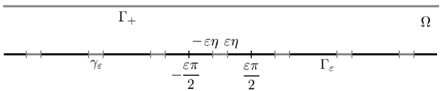
Figure 1: Waveguide with frequently alternating boundary conditions

Theorem 2.1.

Suppose (1.2). Then

$$\|(\mathcal{H}_{\varepsilon}-\mathrm{i})^{-1}-(\mathcal{H}^{(\mu)}-\mathrm{i})^{-1}\|_{L_{2}(\Omega)\to L_{2}(\Omega)}\leqslant C\varepsilon\mu|\ln\varepsilon\mu|,$$ (2.3)

$$\|(\mathcal{H}_{\varepsilon}-\mathrm{i})^{-1}-(\mathcal{H}^{(0)}-\mathrm{i})^{-1}\|_{L_{2}(\Omega)\to W_{2}^{1}(\Omega)}\leqslant C\mu^{1/2},$$ (2.4)

$$\|(\mathcal{H}_{\varepsilon}-\mathrm{i})^{-1}-(\mathcal{H}^{(0)}-\mathrm{i})^{-1}\|_{L_{2}(\Omega)\to L_{2}(\Omega)}\leqslant C\mu,$$ (2.5)

where the constants $C$ are independent of $\varepsilon$ and $\mu$, and $\mu=\mu(\varepsilon)$ was defined in (1.3). There exists a corrector $W=W(x,\varepsilon,\mu)$ defined explicitly by (3.17) such that

$$\|(\mathcal{H}_{\varepsilon}-\mathrm{i})^{-1}-(1+W)(\mathcal{H}^{(\mu)}-\mathrm{i})^{-1}\|_{L_{2}(\Omega)\to W_{2}^{1}(\Omega)}\leqslant C\varepsilon\mu|\ln\varepsilon\mu|,$$ (2.6)

where the constant $C$ is independent of $\varepsilon$ and $\mu$.

The spectrum of the operator $\mathcal{H}^{(0)}$ is purely essential and coincides with $\left[\frac{1}{4},+\infty\right)$. By [RS1, Ch. VIII, Sec. 7, Ths. VIII.23, VIII.24] and Theorem 2.1 we have

Theorem 2.2.

The spectrum of $\mathcal{H}_{\varepsilon}$ converges to that of $\mathcal{H}^{(0)}$. Namely, if $\lambda\not\in\left[\frac{1}{4},+\infty\right)$, then $\lambda\not\in\operatorname{\sigma}(\mathcal{H}_{\varepsilon})$ for $\varepsilon$ small enough. If $\lambda\in\left[\frac{1}{4},+\infty\right)$, then there exists $\lambda_{\varepsilon}\in\operatorname{\sigma}(\mathcal{H}_{\varepsilon})$ so that $\lambda_{\varepsilon}\to\lambda$ as $\varepsilon\to+0$. The convergence of the spectral projectors associated with $\mathcal{H}_{\varepsilon}$ and $\mathcal{H}^{(0)}$

$$\|\mathcal{P}_{(a,b)}(\mathcal{H}_{\varepsilon})-\mathcal{P}_{(a,b)}(\mathcal{H}^{(0)})\|\to 0,\quad\varepsilon\to 0,$$

is valid for $a<b$.

The operator $\mathcal{H}_{\varepsilon}$ is periodic since the sets $\gamma_{\varepsilon}$ and $\Gamma_{\varepsilon}$ are periodic, and we employ the Floquet decomposition to study its spectrum. We denote

$$\Omega_{\varepsilon}:=\left\{x:|x_{1}|<\frac{\varepsilon\pi}{2},\ 0<x_{2}<\pi\right\},$$

$$\mathring{\gamma}_{\varepsilon}:=\partial\Omega_{\varepsilon}\cap\gamma_{\varepsilon},\quad\mathring{\Gamma}_{\varepsilon}:=\partial\Omega_{\varepsilon}\cap\Gamma_{\varepsilon},\quad\mathring{\Gamma}_{\pm}:=\partial\Omega_{\varepsilon}\cap\Gamma_{\pm}.$$

By $\mathring{\mathcal{H}}_{\varepsilon}(\tau)$ we indicate the self-adjoint non-negative operator in $L_{2}(\Omega_{\varepsilon})$ associated with the sesquilinear form

$$\mathring{\mathfrak{h}}_{\varepsilon}(\tau)[u,v]:=\left(\left(\mathrm{i}\frac{\partial}{\partial x_{1}}-\frac{\tau}{\varepsilon}\right)u,\left(\mathrm{i}\frac{\partial}{\partial x_{1}}-\frac{\tau}{\varepsilon}\right)v\right)_{L_{2}(\Omega_{\varepsilon})}+\left(\frac{\partial u}{\partial x_{2}},\frac{\partial v}{\partial x_{2}}\right)_{L_{2}(\Omega_{\varepsilon})}$$

on $\mathring{W}_{2,per}^{1}(\Omega_{\varepsilon},\mathring{\Gamma}_{+}\cup\mathring{\gamma}_{\varepsilon})$, where $\tau\in[-1,1)$. Here $\mathring{W}_{2,per}^{1}(\Omega_{\varepsilon},\mathring{\Gamma}_{+}\cup\mathring{\gamma}_{\varepsilon})$ is the set of the functions in $\mathring{W}_{2}^{1}(\Omega_{\varepsilon},\mathring{\Gamma}_{+}\cup\mathring{\gamma}_{\varepsilon})$ satisfying periodic boundary conditions on the lateral boundaries of $\Omega_{\varepsilon}$. The operator $\mathring{\mathcal{H}}_{\varepsilon}(\tau)$ has a compact resolvent, since it is bounded as that from $L_{2}(\Omega_{\varepsilon})$ into $W_{2}^{1}(\Omega_{\varepsilon})$, and the space $W_{2}^{1}(\Omega_{\varepsilon})$ is compactly embedded into $L_{2}(\Omega_{\varepsilon})$. Hence, the spectrum of $\mathring{\mathcal{H}}_{\varepsilon}(\tau)$ consists of its discrete part only. We denote the eigenvalues of $\mathring{\mathcal{H}}_{\varepsilon}(\tau)$ by $\lambda_{n}(\tau,\varepsilon)$ and arrange them in the ascending order with the multiplicities taking into account

$$\lambda_{1}(\tau,\varepsilon)\leqslant\lambda_{2}(\tau,\varepsilon)\leqslant\ldots\leqslant\lambda_{n}(\tau,\varepsilon)\leqslant\ldots$$

By [3, Lm. 4.1] we know that

$$\operatorname{\sigma}(\mathcal{H}_{\varepsilon})=\operatorname{\sigma_{e}}(\mathcal{H}_{\varepsilon})=\bigcup\limits_{n=1}^{\infty}\{\lambda_{n}(\tau,\varepsilon):\tau\in[-1,1)\},$$

where $\operatorname{\sigma}(\cdot)$ and $\operatorname{\sigma_{e}}(\cdot)$ indicate the spectrum and the essential spectrum of an operator.

By $\mathfrak{L}_{\varepsilon}$ we denote the subspace of $L_{2}(\Omega_{\varepsilon})$ consisting of the functions independent of $x_{1}$, and we shall make use the decomposition

$$L_{2}(\Omega_{\varepsilon})=\mathfrak{L}_{\varepsilon}\oplus\mathfrak{L}_{\varepsilon}^{\bot},$$

where $\mathfrak{L}_{\varepsilon}^{\bot}$ is the orthogonal complement to $\mathfrak{L}_{\varepsilon}$ in $L_{2}(\Omega_{\varepsilon})$. Let $\mathcal{Q}_{\mu}$ be the self-adjoint non-negative operator in $\mathfrak{L}_{\varepsilon}$ associated with the sesquilinear form

$$\mathfrak{q}[u,v]:=\left(\frac{du}{dx_{2}},\frac{dv}{dx_{2}}\right)_{L_{2}(0,\pi)}+\mu u(0)\overline{v(0)}\quad\text{on}\quad\mathring{W}_{2}^{1}((0,\pi),\{\pi\}),$$

i.e., $\mathcal{Q}_{\mu}$ is the operator $-\frac{d^{2}}{dx_{2}^{2}}$ in $L_{2}(0,\pi)$ with the domain consisting of the functions in $W_{2}^{2}(0,\pi)$ satisfying the boundary conditions

$$u(\pi)=0,\quad u^{\prime}(0)-\mu u(0)=0.$$

Our next results are on the uniform resolvent convergence for $\mathring{\mathcal{H}}_{\varepsilon}(\tau)$ and two-terms asymptotics for the first band functions.

Theorem 2.3.

Let $|\tau|<1-\varkappa$, where $0<\varkappa<1$ is a fixed constant and suppose (1.2). Then for sufficiently small $\varepsilon$ the estimate

$$\left\|\left(\mathring{\mathcal{H}}_{\varepsilon}(\tau)-\frac{\tau^{2}}{\varepsilon^{2}}\right)^{-1}-\mathcal{Q}_{\mu}^{-1}\oplus 0\right\|_{L_{2}(\Omega_{\varepsilon})\to L_{2}(\Omega_{\varepsilon})}\leqslant C\varkappa^{-1/2}(\varepsilon^{1/2}\mu+\varepsilon)$$ (2.7)

holds true, where the constant $C$ is independent of $\varepsilon$, $\mu$, and $\varkappa$.

Theorem 2.4.

Let the hypothesis of Theorem 2.3 holds true. Then given any $N$, for $\varepsilon<2\varkappa^{1/2}N^{-1}$ the eigenvalues $\lambda_{n}(\tau,\varepsilon)$, $n=1,\ldots,N$, satisfy the relations

$$\lambda_{n}(\tau,\varepsilon)=\frac{\tau^{2}}{\varepsilon^{2}}+\Lambda_{n}(\mu)+R_{n}(\tau,\varepsilon,\mu),$$ (2.8)

$$|R_{n}(\tau,\varepsilon,\mu)|\leqslant C\varkappa^{-1/2}n^{4}\varepsilon^{1/2}\mu,$$

where $\Lambda_{n}(\mu)$, $n=1,\ldots,N$, are first $N$ eigenvalues of $\mathcal{Q}_{\mu}$, and the constant $C$ is the same as in (2.7). The eigenvalues $\Lambda_{n}(\mu)$ solve the equation

$$\sqrt{\Lambda}\cos\sqrt{\Lambda}\pi+\mu\sin\sqrt{\Lambda}\pi=0,$$ (2.9)

are holomorphic w.r.t. $\mu$, and

$$\Lambda_{n}(\mu)=\left(n-\frac{1}{2}\right)^{2}+\frac{\mu}{\pi\left(n-\frac{1}{2}\right)}+\mathcal{O}(\mu^{2}).$$ (2.10)

Let

$$\theta(\beta):=-\sum\limits_{j=1}^{+\infty}\frac{1}{n\sqrt{4j^{2}-\beta}(2j+\sqrt{4j^{2}-\beta})}.$$ (2.11)

It will be shown in Lemma 5.2 that the function $\theta(\beta)$ is holomorphic in $\beta$ and its Taylor series is

$$\theta(\beta)=-\sum\limits_{j=1}^{+\infty}\frac{(2j-1)!!\zeta(2j+1)}{8^{j}\,j!}\beta^{j-1},$$ (2.12)

where $\zeta$ is the Riemann zeta-function.

Our last main result provides the asymptotic expansion for the bottom of the essential spectrum of $\mathcal{H}_{\varepsilon}$.

Theorem 2.5.

For $\varepsilon$ small enough, the first eigenvalue $\lambda_{1}(\tau,\varepsilon)$ attains its minimum at $\tau=0$,

$$\inf\limits_{\tau\in[-1,1)}\lambda_{1}(\tau,\varepsilon)=\lambda_{1}(0,\varepsilon).$$ (2.13)

The asymptotics

$$\lambda_{1}(0,\varepsilon)=\Lambda(\varepsilon,\mu)+\mathcal{O}(\mu\varepsilon^{-1/2}\mbox{\rm e}^{-2\varepsilon^{-1}}+\varepsilon^{1/2}\eta^{1/2})$$ (2.14)

holds true, where $\Lambda(\varepsilon,\mu)$ is the real solution to the equation

$$\sqrt{\Lambda}\cos\sqrt{\Lambda}\pi+\mu\sin\sqrt{\Lambda\pi}-\varepsilon^{3}\mu\Lambda^{3/2}\theta(\varepsilon^{2}\Lambda)\cos\sqrt{\Lambda}\pi=0$$ (2.15)

satisfying the restriction

$$\Lambda(\varepsilon,\mu)=\Lambda_{1}(\mu)+o(1),\quad\varepsilon\to 0.$$ (2.16)

The function $\Lambda(\varepsilon,\mu)$ is jointly holomorphic w.r.t. $\varepsilon$ and $\mu$ and can be represented as the series

$$\Lambda(\varepsilon,\mu)=\Lambda_{1}(\mu)+\mu^{2}\sum\limits_{j=1}^{+\infty}\varepsilon^{2j+1}K_{2j+1}(\mu)+\mu^{3}\sum\limits_{j=2}^{+\infty}\varepsilon^{2j}K_{2j}(\mu),$$ (2.17)

where the functions $K_{j}(\mu)$ are holomoprhic w.r.t. $\mu$, and, in particular,

$$K_{3}(\mu)=-\frac{\zeta(3)}{4}\frac{\Lambda_{1}^{2}(\mu)}{\pi\Lambda_{1}(\mu)+\mu+\pi\mu^{2}},$$ (2.18)

$$K_{4}(\mu)=0,$$

$$K_{5}(\mu)=-\frac{3\zeta(5)}{64}\frac{\Lambda_{1}^{3}(\mu)}{\pi\Lambda_{1}(\mu)+\mu+\pi\mu^{2}},$$

$$K_{6}(\mu)=\frac{\zeta(3)^{2}}{64}\frac{\Lambda_{1}^{3}(\mu)(2\pi^{2}\Lambda_{1}^{2}(\mu)+7\pi\mu\Lambda_{1}(\mu)+2\pi^{2}\mu^{2}\Lambda_{1}(\mu)+7\mu^{2}+7\pi\mu^{3})}{(\pi\Lambda_{1}(\mu)+\mu+\pi\mu^{2})^{3}}$$

$$K_{7}(\mu)=-\frac{5\zeta(7)}{512}\frac{\Lambda_{1}^{4}(\mu)}{\pi\Lambda_{1}(\mu)+\mu+\pi\mu^{2}},$$

$$K_{8}(\mu)=\frac{3\zeta(3)\zeta(5)}{512}\frac{\Lambda_{1}^{4}(\mu)(2\pi^{2}\Lambda_{1}^{2}(\mu)+9\pi\mu\Lambda_{1}(\mu)+2\pi^{2}\mu^{2}\Lambda_{1}(\mu)+9\mu^{2}+9\mu^{3}\pi)}{(\pi\Lambda_{1}(\mu)+\mu+\pi\mu^{2})^{3}}.$$

The asymptotic expansion for the associated eigenfunction of $\mathring{\mathcal{H}}_{\varepsilon}(0)$ reads as follows,

$$\|\mathring{\psi}(\cdot,\varepsilon)-\mathring{\Psi}_{\varepsilon}\|_{W_{2}^{1}(\Omega_{\varepsilon})}=\mathcal{O}(\mu\mbox{\rm e}^{-2\varepsilon^{-1}}+\varepsilon\eta^{1/2}),$$ (2.19)

where the function $\mathring{\Psi}_{\varepsilon}$ is defined in (5.27).

Remark 2.6.

All other coefficients of (2.17) can be determined recursively by substituting this series and (2.12) into (2.15), expanding then (2.15) in powers of $\varepsilon$, and solving the obtained equations w.r.t. $K_{i}$.

3 Uniform resolvent convergence for $\mathcal{H}_{\varepsilon}$

In this section we prove Theorem 2.1. Given a function $f\in L_{2}(\Omega)$, we denote

$$u_{\varepsilon}:=(\mathcal{H}_{\varepsilon}-\mathrm{i})^{-1}f,\quad u^{(\mu)}:=(\mathcal{H}^{(\mu)}-\mathrm{i})^{-1}f.$$

The main idea of the proof is to construct a special corrector $W=W(x,\varepsilon,\mu)$ with certain properties and to estimate the norms of $v_{\varepsilon}:=u_{\varepsilon}-(1+W)u^{(\mu)}$ and $u^{(\mu)}W$. In fact, the function W reflects the geometry of the alternation of the boundary conditions for $\mathcal{H}_{\varepsilon}$, and this is why it is much simpler to estimate independently $v_{\varepsilon}$ and $u^{(\mu)}W$ than trying to get directly the estimate for $u_{\varepsilon}-u^{(\mu)}$ and $u_{\varepsilon}-u^{(0)}$. Next lemma is the first main ingredient in the proof of Theorem 2.1 and it shows how $W$ is employed.

Lemma 3.1.

Let $W=W(x,\varepsilon,\mu)$ be an $\varepsilon\pi$-periodic in $x_{1}$ function belonging to $C(\overline{\Omega})\cap C^{\infty}(\overline{\Omega}\setminus\{x:x_{2}=0,\,x_{1}=\pm\varepsilon\eta+\varepsilon\pi n,\,n\in\mathds{Z}\})$ satisfying boundary conditions

$$W=-1\quad\text{on}\quad\gamma_{\varepsilon},\qquad\frac{\partial W}{\partial x_{2}}=-\mu\quad\text{on}\quad\Gamma_{\varepsilon},$$ (3.1)

and having differentiable asymptotics

$$W(x,\varepsilon,\mu)=c_{\pm}(\varepsilon,\mu)r_{\pm}^{1/2}\sin\frac{\theta_{\pm}}{2}+\mathcal{O}(\rho_{\pm}),\quad r_{\pm}\to+0.$$ (3.2)

Here $(r_{\pm},\theta_{\pm})$ are polar coordinates centered at $(\pm\varepsilon\eta,0)$ such that the values $\theta_{\pm}=0$ correspond to the points of $\gamma_{\varepsilon}$. Assume also that $\Delta W\in C(\overline{\Omega})$. Then $(1+W)u^{(\mu)}$ belongs to $\mathring{W}_{2}^{1}(\Omega,\Gamma_{+}\cup\gamma_{\varepsilon})$, and

$$\|\nabla v_{\varepsilon} \|_{L_{2}(\Omega)}^{2}+\mathrm{i}\|v_{\varepsilon}\|_{L_{2}(\Omega)}^{2}=(f,v_{\varepsilon}W)_{L_{2}(\Omega)}+(u^{(\mu)}\Delta W,v_{\varepsilon})_{L_{2}(\Omega)}$$ (3.3)

$$-2\mathrm{i}(u^{(\mu)}W,v_{\varepsilon})_{L_{2}(\Omega)}-2(W\nabla u^{(\mu)},\nabla v_{\varepsilon})_{L_{2}(\Omega)}-\mu(u^{(\mu)},Wv_{\varepsilon})_{L_{2}(\Gamma_{\varepsilon})}.$$

Proof.

We write the integral identities for $u_{\varepsilon}$ and $u^{(\mu)}$,

$$(\nabla u_{\varepsilon},\nabla\phi)_{L_{2}(\Omega)}+\mathrm{i}(u_{\varepsilon},\phi)_{L_{2}(\Omega)}=(f,\phi)_{L_{2}(\Omega)}$$ (3.4)

for all $\phi\in\mathring{W}_{2}^{1}(\Omega,\Gamma_{+}\cup\gamma_{\varepsilon})$, and

$$(\nabla u^{(\mu)},\nabla\phi)_{L_{2}(\Omega)}+\mu(u^{(\mu)},\phi)_{L_{2}(\Gamma_{-})}+\mathrm{i}(u^{(\mu)},\phi)_{L_{2}(\Omega)}=(f,\phi)_{L_{2}(\Omega)}$$ (3.5)

for all $\phi\in\mathring{W}_{2}^{1}(\Omega,\Gamma_{+})$. Employing the smoothness of $W$, (3.1), (3.2), and proceeding as in the proof of Lemma 3.2 in [3], we check that $(1+W)\phi\in\mathring{W}_{2}^{1}(\Omega,\Gamma_{+}\cup\gamma_{\varepsilon})$, if $\phi$ belongs to the domain of $\mathcal{H}_{\varepsilon}$ or $\mathcal{H}^{(\mu)}$. Hence, $(1+W)u^{(\mu)}\in\mathring{W}_{2}^{1}(\Omega,\Gamma_{+}\cup\gamma_{\varepsilon})$. Thus,

$$(1+W)v_{\varepsilon}\in\mathring{W}_{2}^{1}(\Omega,\Gamma_{+}\cup\gamma_{\varepsilon}).$$ (3.6)

We take $\phi=(1+W)v_{\varepsilon}$ in (3.5),

$$(\nabla u^{(\mu)}, \nabla(1+W)v_{\varepsilon})_{L_{2}(\Omega)}+\mu(u^{(\mu)},(1+W)v_{\varepsilon})_{L_{2}(\Gamma_{-})}$$

$$+\mathrm{i}(u^{(\mu)},(1+W)v_{\varepsilon})_{L_{2}(\Omega)}=(f,(1+W)v_{\varepsilon})_{L_{2}(\Omega)},$$

$$(\nabla u^{(\mu)}, (1+W)\nabla v_{\varepsilon})_{L_{2}(\Omega)}+\mathrm{i}(u^{(\mu)},(1+W)v_{\varepsilon})_{L_{2}(\Omega)}=$$

$$(f,(1+W)v_{\varepsilon})_{L_{2}(\Omega)}-(\nabla u^{(\mu)},v_{\varepsilon}\nabla W)_{L_{2}(\Omega)}-\mu(u^{(\mu)},(1+W)v_{\varepsilon})_{L_{2}(\Gamma_{-})},$$

$$(\nabla(1+ W)u^{(\mu)},\nabla v_{\varepsilon})_{L_{2}(\Omega)}+\mathrm{i}((1+W)u^{(\mu)},v_{\varepsilon})_{L_{2}(\Omega)}=$$

$$(f,(1+W)v_{\varepsilon})_{L_{2}(\Omega)}-(\nabla u^{(\mu)},v_{\varepsilon}\nabla W)_{L_{2}(\Omega)}$$

$$+(u^{(\mu)}\nabla W,\nabla v_{\varepsilon})_{L_{2}(\Omega)}-\mu(u^{(\mu)},(1+W)v_{\varepsilon})_{L_{2}(\Gamma_{-})}.$$

We deduct (3.4) with $\phi=v_{\varepsilon}$ from the last identity,

$$\|\nabla v_{\varepsilon}\|_{L_{2}(\Omega)}^{2}+\mathrm{i} \|v_{\varepsilon}\|_{L_{2}(\Omega)}^{2}=-(f,Wv_{\varepsilon})_{L_{2}(\Omega)}+(\nabla u^{(\mu)},v_{\varepsilon}\nabla W)_{L_{2}(\Omega)}$$ (3.7)

$$-(u^{(\mu)}\nabla W,\nabla v_{\varepsilon})_{L_{2}(\Omega)}+\mu(u^{(\mu)},(1+W)v_{\varepsilon})_{L_{2}(\Gamma_{-})}.$$

We integrate by parts taking into account (3.1), (3.5), and (3.6),

$$(\nabla u^{(\mu)}, v_{\varepsilon}\nabla W)_{L_{2}(\Omega)}-(u^{(\mu)}\nabla W,\nabla v_{\varepsilon})_{L_{2}(\Omega)}$$

$$=(\nabla u^{(\mu)},v_{\varepsilon}\nabla W)_{L_{2}(\Omega)}+\int\limits_{\Gamma_{\varepsilon}}u^{(\mu)}\frac{\partial W}{\partial x_{2}}\overline{v}_{\varepsilon}\,\mathrm{d}x_{1}+(\mathrm{div}\,u^{(\mu)}\nabla W,v_{\varepsilon})_{L_{2}(\Omega)}$$

$$=2(\nabla u^{(\mu)},v_{\varepsilon}\nabla W)_{L_{2}(\Omega)}-\mu(u^{(\mu)},v_{\varepsilon})_{L_{2}(\Gamma_{\varepsilon})}+(u^{(\mu)}\Delta W,v_{\varepsilon})_{L_{2}(\Omega)},$$

and

$$(\nabla u^{(\mu)}, v_{\varepsilon}\nabla W)_{L_{2}(\Omega)}=(\nabla u^{(\mu)},\nabla Wv_{\varepsilon})_{L_{2}(\Omega)}-(\nabla u^{(\mu)},W\nabla v_{\varepsilon})_{L_{2}(\Omega)}$$

$$\hphantom{v_{\varepsilon}\nabla W)_{L_{2}(\Omega)}}=(f,Wv_{\varepsilon})_{L_{2}(\Omega)}-\mathrm{i}(u^{(\mu)},Wv_{\varepsilon})_{L_{2}(\Omega)}$$

$$\hphantom{v_{\varepsilon}\nabla W)_{L_{2}(\Omega)}=}-\mu(u^{(\mu)},Wv_{\varepsilon})_{L_{2}(\mathring{\Gamma}_{-})}-(\nabla u^{(\mu)},W\nabla v_{\varepsilon})_{L_{2}(\Omega)}.$$

We substitute the obtained identities into (3.7) and this completes the proof. ∎

As it follows from (3.3), to prove the smallness of $v_{\varepsilon}$ in $W_{2}^{1}(\Omega)$-norm, it is sufficient to construct a function $W$ satisfying the hypothesis of Lemma 3.1 so that the quantities $W$ and $\Delta W$ are small in certain sense. This is why we introduce $W$ as a formal asymptotic solution to the equation

$$\Delta W=0\quad\text{in}\quad\Omega,$$ (3.8)

satisfying (3.1), (3.2) and other assumptions of Lemma 3.1. To construct such solution, we shall employ the asymptotic constructions from [4], [25] based on the method of matching of asymptotic expansions [27] and the boundary layer method [37]. We also mention that similar approach was used in [24, Lm. 1] for constructing a different corrector.

First we construct $W$ formally, and after that we shall prove rigourously all the required properties of the constructed corrector. Denote $\xi=(\xi_{1},\xi_{2})=x\varepsilon^{-1}$, $\varsigma^{(j)}=(\varsigma^{(j)}_{1},\varsigma^{(j)}_{2})$, $\varsigma_{1}^{(j)}=(\xi_{1}-\pi j)\eta^{-1}$, $\varsigma^{(j)}_{2}=\xi_{2}\eta^{-1}$. Outside a small neighborhood of $\gamma_{\varepsilon}$ we construct $W$ as a boundary layer

$$W(x,\varepsilon,\mu)=\varepsilon\mu X(\xi).$$

We pass to $\xi$ in (3.8) and let $\eta=0$ in the boundary conditions. It yields a boundary value problem for $X$,

$$\Delta_{\xi}X=0,\quad\xi_{2}>0,\qquad\frac{\partial X}{\partial\xi_{2}}=-1,\quad\xi\in\Gamma^{0}:=\{\xi:\xi_{2}=0\}\setminus\bigcup\limits_{j=-\infty}^{+\infty}\{(\pi j,0)\},$$ (3.9)

where the function $X$ should be $\pi$-periodic in $\xi_{1}$ and decay exponentially as $\xi_{2}\to+\infty$. It was shown in [23] that the required solution to (3.9) is

$$X(\xi):=\operatorname{Re}\ln\sin(\xi_{1}+\mathrm{i}\xi_{2})+\ln 2-\xi_{2}.$$

It was also shown that

$$X\in C^{\infty}(\{\xi:\xi_{2}\geqslant 0,\,\xi\not=(\pi j,0),\,j\in\mathds{Z}\}),$$

and this function satisfies the differentiable asymptotics

$$X(\xi)=\ln|\xi-(\pi j,0)|+\ln 2-\xi_{2}+\mathcal{O}(\xi-(\pi j,0)|^{2}),\quad\xi\to(\pi j,0),\quad j\in\mathds{Z}.$$ (3.10)

In view of the last identity we rewrite the asymptotics for $X$ as $\xi\to(\pi j,0)$ in terms of $\varsigma^{(j)}$,

$$\varepsilon\mu X(\xi)= \varepsilon\mu\big{(}\ln|\xi-(\pi j,0)|+\ln 2-\xi_{2}\big{)}+\mathcal{O}(\varepsilon\mu|\xi-(\pi j,0)|^{2})$$ (3.11)

$$= -1+\varepsilon\mu\big{(}\ln|\varsigma^{(j)}|+\ln 2\big{)}-\varepsilon\mu\eta\varsigma^{(j)}_{2}+\mathcal{O}(\varepsilon\mu\eta^{2}|\varsigma^{(j)}|^{2}).$$

In accordance with the method of matching of asymptotic expansions it follows from the obtained identities that in a small neighborhood of each interval of $\gamma_{\varepsilon}$ we should construct $W$ as an internal layer,

$$W(x,\varepsilon,\mu)=-1+\varepsilon\mu W_{in}^{(j)}(\varsigma^{(j)}),$$ (3.12)

where

$$W_{in}^{(j)}(\varsigma^{(j)})=\ln|\varsigma^{(j)}|+\ln 2+o(1),\quad\varsigma^{(j)}\to+\infty.$$ (3.13)

We substitute (3.12) into (3.8), (3.1), which leads us to the boundary value problem for $W_{in}^{(j)}$,

$$\Delta_{\varsigma^{(j)}}W_{in}^{(j)}=0,\quad\varsigma_{2}^{(j)}>0,$$ (3.14)

$$W_{in}^{(j)}=0,\quad\varsigma^{(j)}\in\gamma^{1},\qquad\frac{\partial W_{in}^{(j)}}{\partial\varsigma_{2}^{(j)}}=0,\quad\varsigma^{(j)}\in\Gamma^{1},$$

$$\gamma^{1}:=\{\varsigma:\,|\varsigma_{1}|<1,\,\varsigma_{2}=0\},\quad\Gamma^{1}:=O\varsigma_{1}\setminus\overline{\gamma}^{1}.$$

It was shown in [23] that the problem (3.13), (3.14) is solvable and

$$W_{in}^{(j)}(\varsigma^{(j)})=Y(\varsigma^{(j)}),\quad Y(\varsigma):=\operatorname{Re}\ln(z+\sqrt{z^{2}-1}),\quad z=\varsigma_{1}+\mathrm{i}\varsigma_{2},$$ (3.15)

where the branch of the root is fixed by the requirement $\sqrt{1}=1$. It was also shown that

$$Y(\varsigma)=\ln|\varsigma|+\ln 2+\mathcal{O}(|\varsigma|^{-2}),\quad\varsigma\to\infty.$$ (3.16)

As it follows from the last asymptotics, the term $-\varepsilon\mu\varsigma_{2}^{(j)}$ in (3.11) is not matched with any term in the boundary layer. At the same time, it was found in [4], [24], [25] that such terms should be either matched or cancelled out to obtain a reasonable estimate for the error terms. This is also the case in our problem. In contrast to [4], [24], [25], to solve this issue we shall not construct additional terms in $W$, but employ a different trick to solve this issue. Namely, we add the function $\varepsilon\mu\xi_{2}$ to the boundary layer and add also $-\mu x_{2}$ as the external expansion. It changes neither equations nor boundary conditions for $W$ but allows us to cancel out the mentioned term in (3.11). The final form of $W$ is as follows,

$$W(x,\varepsilon,\mu)= -\mu x_{2}+\varepsilon\mu(X(\xi)+\xi_{2})\prod\limits_{j=-\infty}^{+\infty}\Big{(}1-\chi_{1}\big{(}|\varsigma^{(j)}|\eta^{\alpha}\big{)}\Big{)}$$ (3.17)

$$+\sum\limits_{j=-\infty}^{+\infty}\chi_{1}\big{(}|\varsigma^{(j)}|\eta^{\alpha}\big{)}\big{(}-1+\varepsilon\mu Y(\varsigma^{(j)})\big{)},$$

where $\alpha\in(0,1)$ is a constant, which will be chosen later, and $\chi_{1}=\chi_{1}(t)$ is an infinitely differentiable cut-off function taking values in $[0,1]$, being one as $t<1$, and vanishing as $t>3/2$. It can be easily seen that the sum and the product in the definition of (3.17) are always finite.

Let us check that the function $W$ satisfies the hypothesis of Lemma 3.1. By direct calculations we check that the function $W$ is $\varepsilon\pi$-periodic w.r.t. $x_{1}$, belongs to $C(\overline{\Omega})\cap C^{\infty}(\overline{\Omega}\setminus\{x:x_{2}=0,\,x_{1}=\pm\varepsilon\eta+\varepsilon\pi n,\,n\in\mathds{Z}\})$, and satisfies (3.2). The boundary condition on $\gamma_{\varepsilon}$ in (3.1) is obviously satisfied. Taking into account the boundary conditions (3.9), (3.13), we check

$$\frac{\partial W}{\partial x_{2}}\Big{|}_{x\in\Gamma_{\varepsilon}}= -\mu+\varepsilon\mu\left(\frac{\partial X}{\partial\xi_{2}}\Big{|}_{\xi\in\Gamma^{0}}+1\right)\prod\limits_{j=-\infty}^{+\infty}\big{(}1-\chi_{1}(|\varsigma^{(j)}|\eta^{\alpha})\big{)}$$

$$+\varepsilon\mu\sum\limits_{j=-\infty}^{+\infty}\chi_{1}\big{(}|\varsigma^{(j)}|\eta^{\alpha}\big{)}\frac{\partial Y}{\partial\varsigma_{2}^{(j)}}\Big{|}_{\varsigma^{(j)}\in\Gamma^{1}}=-\mu,$$

i.e., the boundary condition on $\Gamma_{\varepsilon}$ in (3.1) is satisfied, too.

Let us calculate $\Delta W$. In order to do it, we employ the equations in (3.9), (3.13),

$$\Delta W(x)=2\sum\limits_{j=-\infty}^{+\infty}\nabla_{x}\chi_{1}\big{(}|\varsigma^{(j)}|\eta^{\alpha}\big{)}\cdot\nabla_{x}W_{mat}^{(j)}(x,\varepsilon,\mu)$$ (3.18)

$$\hphantom{\Delta W(x)=}+\sum\limits_{j=-\infty}^{+\infty}W_{mat}^{(j)}(x,\varepsilon,\mu)\Delta_{x}\chi_{1}\big{(}|\varsigma^{(j)}|\eta^{\alpha}\big{)},$$

$$W_{mat}^{(j)}(x,\varepsilon,\mu)=-1+\varepsilon\mu\big{(}Y(\varsigma^{(j)})-X(\xi)-\xi_{2}\big{)}.$$

It follows from the definition of $\xi$, $\varsigma^{(j)}$, $\chi_{1}$, $X$, $Y$, and the last formula that $\Delta W\in C^{\infty}(\overline{\Omega})$. Thus, we can apply Lemma 3.1. To estimate the right hand side of (3.3) we need two auxiliary lemmas.

Given any $\delta\in(0,\pi/2)$, denote

$$\Omega^{\delta}:=\bigcup\limits_{j=-\infty}^{+\infty}\Omega_{j}^{\delta},\quad\Omega_{j}^{\delta}:=\{x:|x-(\pi j,0)|<\varepsilon\delta\}\cap\Omega.$$

Lemma 3.2.

For any $u\in W_{2}^{1}(\Omega)$ and any $\delta\in(0,\pi/4)$ the inequality

$$\|u\|_{L_{2}(\Omega^{\delta})}\leqslant C\delta\big{(}|\ln\delta|^{1/2}+1\big{)}\|u\|_{W_{2}^{1}(\Omega)}$$ (3.19)

holds true, where the constant $C$ is independent of $\delta$ and $u$.

Proof.

We begin with the formulas

$$\|u\|_{L_{2}(\Omega^{\delta})}^{2}=\sum\limits_{j=-\infty}^{+\infty}\|u\|_{L_{2}(\Omega_{j}^{\delta})}^{2},$$ (3.20)

$$\|u\|_{L_{2}(\Omega_{j}^{\delta})}^{2}=\int\limits_{\Omega_{j}^{\delta}}|u(x)|^{2}\,\mathrm{d}x=\varepsilon^{2}\int\limits_{|\xi-(\pi j,0)|<\delta,\,\xi_{2}>0}|u(\varepsilon\xi)|^{2}\,\mathrm{d}\xi$$

$$\hphantom{\|u\|_{L_{2}(\Omega_{j}^{\delta})}^{2}}=\varepsilon^{2}\int\limits_{|\xi-(\pi j,0)|<\delta,\,\xi_{2}>0}|\chi_{2}(\xi-(\pi j,0))u(\varepsilon\xi)|^{2}\,\mathrm{d}\xi,$$

where $\chi_{2}=\chi_{2}(\xi)$ is an infinitely differentiable function being one as $|\xi|<\delta$ and vanishing as $|\xi|>\pi/3$. We also suppose that the functions $\chi_{2}$, $\chi_{2}^{\prime}$ are bounded uniformly in $\xi$ and $\delta$. Hence,

$$\chi_{2}(\cdot-(\pi j,0))u\in\mathring{W}_{2}^{1}(\Pi_{j}^{1},\partial\Pi_{j}^{1}),\quad\Pi_{j}^{1}:=\left\{\xi:\,|\xi_{1}-\pi j|<\frac{\pi}{2},\,0<\xi_{2}<1\right\}.$$

By [28, Lm. 3.2], we obtain

$$\varepsilon^{2} \int\limits_{|\xi-(\pi j,0)|<\delta,\,\xi_{2}>0}|\chi_{2}u|^{2}\,\mathrm{d}\xi\leqslant C\varepsilon^{2}\delta^{2}(|\ln\delta|+1)\int\limits_{\Pi_{j}^{1}}\big{(}|\nabla_{\xi}\chi_{2}u|^{2}+|\chi_{2}u|^{2}\big{)}\,\mathrm{d}\xi$$

$$\leqslant C\varepsilon^{2}\delta^{2}(|\ln\delta|+1)\big{(}\|\nabla_{\xi}u\|_{L_{2}(\Pi_{j}^{1})}+\|u\|_{L_{2}(\Pi_{j}^{1})}\big{)}$$

$$\leqslant C\delta^{2}(|\ln\delta|+1)\|u\|_{W_{2}^{1}(\{x:|x_{1}-\varepsilon\pi j|<\varepsilon\pi/2,0<x_{2}<\pi\})}^{2},$$

where the constants $C$ are independent of $j$, $\varepsilon$, $\delta$, $\mu$, and $u$. We substitute these inequalities into (3.20) and arrive at (3.19). ∎

Lemma 3.3.

For any $u\in W_{2}^{2}(\Omega)$ and any $\delta\in(0,\pi/2)$ the inequality

$$\|u\|_{L_{2}(\gamma_{\varepsilon}^{\delta})}\leqslant C\delta^{1/2}\|u\|_{W_{2}^{2}(\Omega)},\quad\gamma_{\varepsilon}^{\delta}:=\{x:|x_{1}-\varepsilon\pi j|<\varepsilon\delta,\,x_{2}=0\},$$

holds true, where the constant $C$ is independent of $\varepsilon$, $\delta$, and $u$.

Proof.

It is clear that

$$\|u\|_{L_{2}(\gamma_{\varepsilon}^{\delta})}=\sum\limits_{j=-\infty}^{+\infty}\|u\|_{L_{2}(\gamma_{\varepsilon,j}^{\delta})},\quad\gamma_{\varepsilon,j}^{\delta}:=\left\{x:|x_{1}-\varepsilon\pi j|<\varepsilon\delta,\,x_{2}=0\right\}.$$ (3.21)

It follows from the definition of $\chi_{2}$ (see the proof of Lemma 3.2) that

$$\|u\|_{L_{2}(\gamma_{\varepsilon,j}^{\delta})}^{2}=\int\limits_{\gamma_{\varepsilon,j}^{\delta}}\left|\chi_{2}\left(\frac{x_{1}}{\varepsilon}-\pi j\right)u(x_{1},0)\right|^{2}\,\mathrm{d}x_{1}.$$ (3.22)

Since

$$\chi_{2}\left(\frac{x_{1}}{\varepsilon}-\pi j\right)u(x_{1},0)=\int\limits_{\varepsilon\pi j-\frac{\varepsilon\pi}{2}}^{x_{1}}\frac{\partial}{\partial x_{1}}\left(\chi_{2}\left(\frac{x_{1}}{\varepsilon}-\pi j\right)u(x_{1},0)\right)\,\mathrm{d}x_{1},$$

by the Cauchy-Schwartz inequality we get

$$\frac{\partial}{\partial x_{1}}\left(\chi_{2}\left(\frac{x_{1}}{\varepsilon}-\pi j\right)u(x_{1},0)\right)=\chi_{2}\left(\frac{x_{1}}{\varepsilon}-\pi j\right)\frac{\partial u}{\partial x_{1}}(x_{1},0)+\varepsilon^{-1}\chi_{2}^{\prime}\left(\frac{x_{1}}{\varepsilon}-\pi j\right)u(x_{1}),$$

$$\left|\chi_{2}\left(\frac{x_{1}}{\varepsilon}-\pi j,0\right)u(x_{1},0)\right|^{2}\leqslant C\left(\varepsilon\int\limits_{\gamma_{\varepsilon,j}}\left|\frac{\partial u}{\partial x_{1}}(x_{1},0)\right|^{2}\,\mathrm{d}x_{1}+\varepsilon^{-1}\int\limits_{\gamma_{\varepsilon,j}}|u(x_{1},0)|^{2}\,\mathrm{d}x_{1}\right),$$

$$\gamma_{\varepsilon,j}:=\left\{x:|x_{1}-\varepsilon\pi j|<\frac{\varepsilon\pi}{2},\,x_{2}=0\right\},$$

where the constants $C$ are independent of $j$, $\varepsilon$, $\delta$, and $u$. The last estimate and (3.22) imply

$$\|u\|_{L_{2}(\gamma_{\varepsilon,j}^{\delta})}^{2}\leqslant C\delta\left(\Big{\|}\frac{\partial u}{\partial x_{1}}\Big{\|}_{L_{2}(\gamma_{\varepsilon,j})}^{2}+\|u\|_{L_{2}(\gamma_{\varepsilon,j})}^{2}\right),$$

where the constant $C$ is independent of $j$, $\varepsilon$, $\delta$, and $u$. We substitute the obtained inequality into (3.21) and employ the standard embedding of $W_{2}^{2}(\Omega)$ into $W_{2}^{1}(\Gamma_{-})$ that completes the proof. ∎

Lemma 3.4.

The estimates

$$|\Delta W|\leqslant C\varepsilon^{-1}\mu(1+\eta^{4\alpha-2}), x\in\Omega,$$ (3.23)

$$|W|\leqslant C\varepsilon\mu(|\ln\delta|+1), x\in\Omega\setminus\Omega^{\delta}, \frac{3}{2}\eta^{\alpha}<\delta<\frac{\pi}{2},$$ (3.24)

$$|W|\leqslant C, x\in\Omega^{\delta}, \frac{3}{2}\eta^{\alpha}<\delta<\frac{\pi}{2},$$ (3.25)

are valid, where the constants $C$ are independent of $\varepsilon$, $\mu$, $\eta$, $\delta$, and $x$.

Proof.

Since $W$ is $\varepsilon\pi$-periodic w.r.t. $x_{1}$, it is sufficient to prove the estimates only for $|x_{1}|<\varepsilon\pi/2$, $0<x_{2}<\pi$. It follows directly from the definition of $X$, $Y$, and (3.13), (3.16) that for any $\delta\in(0,\pi/2)$

$$|X(\xi)|\leqslant C\big{(}|\ln\delta|+1\big{)},\quad|\xi_{1}|<\frac{\pi}{2},\quad\xi_{2}>0,\quad|\xi|\geqslant\delta,$$

$$|Y(\varsigma)|\leqslant C\big{(}|\ln\delta\eta^{-1}|+1\big{)}\leqslant C\big{(}|\ln\delta|+\varepsilon^{-1}\mu^{-1}\big{)},\quad|\varsigma|\leqslant\delta\eta^{-1},$$

where the constants $C$ are independent of $\varepsilon$, $\mu$, $\eta$, $\delta$, and $x$. These estimates and (3.17) imply (3.24), (3.25).

It follows from the definition of $\chi_{1}$ that $\Delta W$ is non-zero only as

$$\eta^{-\alpha}<|\varsigma^{(1)}|<\frac{3}{2}\eta^{-\alpha}.$$

For the corresponding values of $x$ due to (3.13), (3.15) the differentiable asymptotics

$$W_{mat}^{(1)}(x,\varepsilon,\mu)=\mathcal{O}\big{(}\varepsilon\mu(|\varsigma^{(1)}|^{-2}+|\xi|^{2})\big{)},\quad\eta^{-\alpha}<|\varsigma^{(1)}|<\frac{3}{2}\eta^{-\alpha},\quad\eta^{1-\alpha}<|\xi|<\frac{3}{2}\eta^{1-\alpha},$$

holds true. Hence, for the same values of $\xi$ and $\varsigma^{(1)}$

$$W_{mat}^{(1)}=\mathcal{O}\big{(}\varepsilon\mu(\eta^{2\alpha}+\eta^{2-2\alpha})\big{)},$$

$$\nabla_{x}W_{mat}^{(1)}=\mathcal{O}\big{(}\mu(\eta^{-1}|\varsigma^{(1)}|^{-3}+|\xi|)\big{)}=\mathcal{O}\big{(}\mu(\eta^{1-\alpha}+\eta^{3\alpha-1})\big{)}.$$

Substituting the identities obtained into (3.18) and taking into account the relations

$$\nabla_{x}\chi_{1}\big{(}|\varsigma^{(j)}|\eta^{\alpha}\big{)}=\mathcal{O}(\varepsilon^{-1}\eta^{\alpha-1}),\quad\Delta_{x}\chi_{1}\big{(}|\varsigma^{(j)}|\eta^{\alpha}\big{)}=\mathcal{O}(\varepsilon^{-2}\eta^{2\alpha-2}),$$

we arrive at (3.23). ∎

Let us estimate the right hand side of (3.3). We have

$$|(f,Wv_{\varepsilon})_{L_{2}(\Omega)}|\leqslant\|f\|_{L_{2}(\Omega)}\|Wv_{\varepsilon}\|_{L_{2}(\Omega)},$$

$$\|Wv_{\varepsilon}\|_{L_{2}(\Omega)}^{2}=\|Wv_{\varepsilon}\|_{L_{2}(\Omega\setminus\Omega^{\delta})}^{2}+\|Wv_{\varepsilon}\|_{L_{2}(\Omega^{\delta})}^{2}.$$ (3.26)

Let $\delta\in\left(\frac{3}{2}\eta^{\alpha},\frac{\pi}{2}\right)$. Applying Lemma 3.2 and using (3.24), (3.25), we have

$$\|v_{\varepsilon}W\|_{L_{2}(\Omega\setminus\Omega^{\delta})}^{2}\leqslant C\varepsilon^{2}\mu^{2}(|\ln\delta|^{2}+1)\|v_{\varepsilon}\|_{L_{2}(\Omega\setminus\Omega^{\delta})}^{2},$$ (3.27)

$$\|v_{\varepsilon}W\|_{L_{2}(\Omega^{\delta})}^{2}\leqslant C\delta^{2}(|\ln\delta|+1)\|v_{\varepsilon}\|_{W_{2}^{1}(\Omega)}^{2}.$$

Here and till the end of this section we indicate by $C$ various non-essential constants independent of $\varepsilon$, $\mu$, $\eta$, $\delta$, $x$, $v_{\varepsilon}$, $u^{(\mu)}$, and $f$. The inequalities (3.27) yield

$$|(f,v_{\varepsilon}W)_{L_{2}(\Omega)}|\leqslant C\big{(}\varepsilon\mu|\ln\delta|+\delta|\ln\delta|^{1/2}+\delta\big{)}\|v_{\varepsilon}\|_{W_{2}^{1}(\Omega)}\|f\|_{L_{2}(\Omega)}.$$ (3.28)

It follows from the definition of $u^{(\mu)}$ that

$$\|u^{(\mu)}\|_{W_{2}^{2}(\Omega)}\leqslant C\|f\|_{L_{2}(\Omega)}.$$ (3.29)

Taking into account this inequality, we proceed in the same way as in (3.26), (3.27), (3.28),

$$\begin{aligned} \|u^{(\mu)}W\|_{L_{2}(\Omega)}&\leqslant C(\varepsilon\mu|\ln\delta|+\delta|\ln\delta|^{1/2}+\delta)\|u^{(\mu)}\|_{W_{2}^{1}(\Omega)}\\ &\leqslant C(\varepsilon\mu|\ln\delta|+\delta|\ln\delta|^{1/2}+\delta)\|f\|_{L_{2}(\Omega)},\end{aligned}$$ (3.30)

$$\begin{aligned} \|W\nabla u^{(\mu)}\|_{L_{2}(\Omega)}&\leqslant C(\varepsilon\mu|\ln\delta|+\delta|\ln\delta|^{1/2}+\delta)\|u^{(\mu)}\|_{W_{2}^{2}(\Omega)}\\ &\leqslant C(\varepsilon\mu|\ln\delta|+\delta|\ln\delta|^{1/2}+\delta)\|f\|_{L_{2}(\Omega)},\end{aligned}$$ (3.31)

$$\begin{aligned} \big{|}(u^{(\mu)},Wv_{\varepsilon})_{L_{2}(\Omega)}+&(\nabla u^{(\mu)},W\nabla v_{\varepsilon})_{L_{2}(\Omega)}\big{|}\\ &\leqslant\|u^{(\mu)}W\|_{L_{2}(\Omega)}\|v_{\varepsilon}\|_{L_{2}(\Omega)}+\|W\nabla u^{(\mu)}\|_{L_{2}(\Omega)}\|\nabla v_{\varepsilon}\|_{L_{2}(\Omega)}\\ &\leqslant C(\varepsilon\mu|\ln\delta|+\delta|\ln\delta|^{1/2}+\delta)\|f\|_{L_{2}(\Omega)}\|v_{\varepsilon}\|_{W_{2}^{1}(\Omega)}.\end{aligned}$$ (3.32)

Employing (3.23) instead of (3.24), (3.25), and applying then Lemma 3.2 with $\delta=\eta^{\alpha}$, we get

$$\|u^{(\mu)}\Delta W\|_{L_{2}(\Omega)}=\|u^{(\mu)}\Delta W\|_{L_{2}(\Omega_{2\eta^{\alpha}})} \leqslant C\eta^{\alpha}\varepsilon^{-3/2}\mu^{1/2}(1+\eta^{4\alpha-2})\|u^{(\mu)}\|_{W_{2}^{1}(\Omega)}$$ (3.33)

$$\leqslant C\eta^{\alpha}\varepsilon^{-3/2}\mu^{1/2}(1+\eta^{4\alpha-2})\|f\|_{L_{2}(\Omega)}.$$

Using (3.24), (3.25), (3.28), Lemma 3.3 with $\delta=\widetilde{\delta}\in(\eta^{\alpha},\pi/2)$, the embedding of $W_{2}^{2}(\Omega)$ in $W_{2}^{1}(\Gamma_{-})$, and proceeding as in (3.26), (3.27), (3.28), we obtain

$$\big{|}(u^{(\mu)},Wv_{\varepsilon})_{L_{2}(\Gamma_{\varepsilon})}\big{|}\leqslant\|u^{(\mu)}W\|_{L_{2}(\Gamma_{\varepsilon})}\|v_{\varepsilon}\|_{L_{2}(\Gamma_{-})}\leqslant C\|u^{(\mu)}W\|_{L_{2}(\Gamma_{\varepsilon})}\|v_{\varepsilon}\|_{W_{2}^{1}(\Omega)},$$

$$\begin{aligned} &\|u^{(\mu)}W\|_{L_{2}(\Gamma_{\varepsilon})}^{2}=\|u^{(\mu)}W\|_{L_{2}(\Gamma_{\varepsilon}\setminus\gamma_{\varepsilon}^{\widetilde{\delta}})}^{2}+\|u^{(\mu)}W\|_{L_{2}(\gamma_{\varepsilon}^{\widetilde{\delta}})}^{2}\\ &\hphantom{\|u^{(\mu)}W\|_{L_{2}(\Gamma_{\varepsilon})}^{2}}\leqslant C\varepsilon^{2}\mu^{2}(|\ln\widetilde{\delta}|^{2}+1)\|u^{(\mu)}\|_{L_{2}(\Gamma_{\varepsilon})}^{2}+C\widetilde{\delta}\|u^{(\mu)}\|_{W_{2}^{2}(\Omega)}^{2}\\ &\hphantom{\|u^{(\mu)}W\|_{L_{2}(\Gamma_{\varepsilon})}^{2}}\leqslant C\big{(}\widetilde{\delta}+\varepsilon^{2}\mu^{2}(|\ln\widetilde{\delta}|^{2}+1)\big{)}\|f\|_{L_{2}(\Omega)}^{2},\end{aligned}$$ (3.34)

$$\big{|}(u^{(\mu)},Wv_{\varepsilon})_{L_{2}(\Gamma_{\varepsilon})}\big{|}\leqslant C\big{(}\widetilde{\delta}^{1/2}+\varepsilon\mu(|\ln\widetilde{\delta}|+1)\big{)}\|f\|_{L_{2}(\Omega)},$$

Let $\alpha\in(1/2,1)$. The last obtained estimate, (3.28), (3.32), (3.33), and (3.3) yield

$$\|v_{\varepsilon}\|_{W_{2}^{1}(\Omega)}^{2}\leqslant C(\delta|\ln\delta|^{1/2}+\varepsilon\mu|\ln\delta|+\varepsilon\mu^{2}|\ln\widetilde{\delta}|+\mu\widetilde{\delta}^{1/2})\|f\|_{L_{2}(\Omega)}\|v_{\varepsilon}\|_{W_{2}^{1}(\Omega)},$$

and it is assumed here that

$$\eta^{\alpha}<\delta<\pi/2,\quad\eta^{\alpha}<\widetilde{\delta}<\pi/2,\quad\delta=\delta(\varepsilon)\to+0,\quad\widetilde{\delta}=\widetilde{\delta}(\varepsilon)\to+0\quad\text{as}\quad\varepsilon\to+0.$$

Thus, taking $\delta=\varepsilon\mu$, $\widetilde{\delta}=\varepsilon^{2}\mu^{2}$, we get

$$\|v_{\varepsilon}\|_{W_{2}^{1}(\Omega)}\leqslant C\varepsilon\mu|\ln\varepsilon\mu|\|f\|_{L_{2}(\Omega)},$$

and it proves (2.6).

We take $\delta=\varepsilon\mu$ in (3.30) and employ (2.6),

$$\|(\mathcal{H}_{\varepsilon}- \mathrm{i})^{-1}f-(\mathcal{H}^{(\mu)}-\mathrm{i})^{-1}f\|_{L_{2}(\Omega)}=\|u_{\varepsilon}-u^{(\mu)}\|_{L_{2}(\Omega)}$$

$$\leqslant\|u_{\varepsilon}-(1+W)u^{(\mu)}\|_{L_{2}(\Omega)}+\|u^{(\mu)}W\|_{L_{2}(\Omega)}$$

$$\leqslant C\varepsilon\mu|\ln\varepsilon\mu|\|f\|_{L_{2}(\Omega)},$$

which proves (2.3).

Lemma 3.5.

The estimate

$$\|\nabla(u^{(\mu)}W)\|_{L_{2}(\Omega)}\leqslant C\mu^{1/2}\|f\|_{L_{2}(\Omega)}$$ (3.35)

holds true.

Proof.

We integrate by parts employing (3.1), (3.2), (2.1), (2.2),

$$\|\nabla(u^{(\mu)}W)\|_{L_{2}(\Omega)}^{2}= -\left(\frac{\partial}{\partial x_{2}}u^{(\mu)}W,u^{(\mu)}W\right)_{L_{2}(\Gamma_{-})}-\left(\Delta(u^{(\mu)}W),u^{(\mu)}W\right)_{L_{2}(\Omega)}$$

$$= -\mu\|u^{(\mu)}W\|_{L_{2}(\Gamma_{-})}^{2}+\int\limits_{\gamma_{\varepsilon}}|u^{(\mu)}|^{2}\frac{\partial W}{\partial x_{2}}\,\mathrm{d}x_{1}+\mu(u^{(\mu)},u^{(\mu)}W)_{L_{2}(\Gamma_{\varepsilon})}$$

$$-(W\Delta u^{(\mu)},Wu^{(\mu)})_{L_{2}(\Omega)}-2\left(W\nabla u^{(\mu)},u^{(\mu)}\nabla W\right)_{L_{2}(\Omega)}$$

$$-\left(u^{(\mu)}\Delta W,u^{(\mu)}W\right)_{L_{2}(\Omega)}.$$

We take the real part of this identity,

$$\|\nabla(u^{(\mu)}W)\|_{L_{2}(\Omega)}^{2} =\mu(u^{(\mu)},u^{(\mu)}W)_{L_{2}(\Gamma_{\varepsilon})}+\int\limits_{\gamma_{\varepsilon}}|u^{(\mu)}|^{2}\frac{\partial W}{\partial x_{2}}\,\mathrm{d}x_{1}$$ (3.36)

$$-\mu\|u^{(\mu)}W\|_{L_{2}(\Gamma_{-})}^{2}-\operatorname{Re}(W\Delta u^{(\mu)},Wu^{(\mu)})_{L_{2}(\Omega)}$$

$$-2\operatorname{Re}\left(W\nabla u^{(\mu)},u^{(\mu)}\nabla W\right)_{L_{2}(\Omega)}-\left(u^{(\mu)}\Delta W,u^{(\mu)}W\right)_{L_{2}(\Omega)}.$$

Let us calculate the fifth term in the right hand side of the last equation. We integrate by parts employing (2.1),

$$2\operatorname{Re}\left(W\nabla u^{(\mu)},u^{(\mu)}\nabla W\right)_{L_{2}(\Omega)}= \frac{1}{2}\int\limits_{\Omega}\nabla W^{2}\cdot\nabla|u^{(\mu)}|^{2}\,\mathrm{d}x$$

$$= -\frac{1}{2}\int\limits_{\Gamma_{-}}W^{2}\frac{\partial}{\partial x_{2}}|u^{(\mu)}|^{2}\,\mathrm{d}x_{1}-\frac{1}{2}\int\limits_{\Omega}W^{2}\Delta|u^{(\mu)}|^{2}\,\mathrm{d}x$$

$$= -\mu\|u^{(\mu)}W\|_{L_{2}(\Gamma_{-})}^{2}-\operatorname{Re}(Wu^{(\mu)},W\Delta u^{(\mu)})_{L_{2}(\Omega)}$$

$$-\|W\nabla u^{(\mu)}\|_{L_{2}(\Omega)}^{2}.$$

We substitute the last identity into (3.36),

$$\|\nabla(u^{(\mu)}W)\|_{L_{2}(\Omega)}^{2}= \mu(u^{(\mu)},u^{(\mu)}W)_{L_{2}(\Gamma_{\varepsilon})}+\int\limits_{\gamma_{\varepsilon}}|u^{(\mu)}|^{2}\frac{\partial W}{\partial x_{2}}\,\mathrm{d}x_{1}$$ (3.37)

$$+\|W\nabla u^{(\mu)}\|_{L_{2}(\Omega)}^{2}-\left(u^{(\mu)}\Delta W,u^{(\mu)}W\right)_{L_{2}(\Omega)}.$$

Taking $\delta=\varepsilon\mu$ in (3.31), we get

$$\|W\nabla u^{(\mu)}\|_{L_{2}(\Omega)}\leqslant C\varepsilon\mu|\ln\varepsilon\mu|\|f\|_{L_{2}(\Omega)}.$$ (3.38)

It follows from (3.30) with $\delta=\varepsilon\mu$ and (3.33) that

$$\big{|}(u^{(\mu)}\Delta W,u^{(\mu)}W)_{L_{2}(\Omega)}\big{|}\leqslant C\eta^{\alpha}\varepsilon^{-1/2}\mu^{3/2}|\ln\varepsilon\mu|\|f\|_{L_{2}(\Omega)}^{2},\quad\alpha\in(1/2,1).$$ (3.39)

Employing (3.17), (3.15), by direct calculations we check that

$$\int\limits_{\gamma_{\varepsilon}}|u^{(\mu)}|^{2}\frac{\partial W}{\partial x_{2}}\,\mathrm{d}x_{1}= \sum\limits_{j=-\infty}^{+\infty}\int\limits_{\gamma_{\varepsilon,j}}|u^{(\mu)}|^{2}\frac{\partial W}{\partial x_{2}}\,\mathrm{d}x_{1}$$

$$= \varepsilon\mu\sum\limits_{j=-\infty}^{+\infty}\int\limits_{\gamma_{\varepsilon,j}}|u^{(\mu)}|^{2}\frac{\partial}{\partial x_{1}}\arcsin\frac{x_{1}-\varepsilon\pi j}{\varepsilon\eta}\,\mathrm{d}x_{1},$$

and

$$\int\limits_{\gamma_{\varepsilon,j}}|u^{(\mu)}|^{2}\frac{\partial}{\partial x_{1}}\arcsin\frac{x_{1}-\varepsilon\pi j}{\varepsilon\eta}\,\mathrm{d}x_{1}=\int\limits_{\varepsilon\pi j-\varepsilon\eta}^{\varepsilon\pi j}|u^{(\mu)}|^{2}\frac{\partial}{\partial x_{1}}\left(\arcsin\frac{x_{1}-\varepsilon\pi j}{\varepsilon\eta}+\frac{\pi}{2}\right)\,\mathrm{d}x_{1}$$

$$\hphantom{\int\limits_{\gamma_{\varepsilon}^{j}}|u^{(\mu)}|^{2}=}+\int\limits_{\varepsilon\pi j}^{\varepsilon\pi j+\varepsilon\eta}|u^{(\mu)}|^{2}\frac{\partial}{\partial x_{1}}\left(\arcsin\frac{x_{1}-\varepsilon\pi j}{\varepsilon\eta}-\frac{\pi}{2}\right)\,\mathrm{d}x_{1},$$

$$\hphantom{\int\limits_{\gamma_{\varepsilon}^{j}}|u^{(\mu)}|^{2}}=\pi|u^{(\mu)}(\varepsilon\pi j,0)|^{2}+\int\limits_{\gamma_{\varepsilon,j}}\left(\arcsin\frac{x_{1}-\varepsilon\pi j}{\varepsilon\eta}-\frac{\pi}{2}\operatorname{sgn}(x_{1}-\varepsilon\pi j)\right)\frac{\partial}{\partial x_{1}}|u^{(\mu)}|^{2}\,\mathrm{d}x_{1},$$

where

$$\pi|u^{(\mu)}(\varepsilon\pi j,0)|^{2}=\frac{1}{\varepsilon}\int\limits_{\varepsilon\pi(j-1)}^{\varepsilon\pi j}\frac{\partial}{\partial x_{1}}\big{(}(x_{1}-\varepsilon\pi(j-1))|u^{(\mu)}|^{2}\big{)}\,\mathrm{d}x_{1}.$$

Thus, in view of the embedding of $W_{2}^{2}(\Omega)$ into $W_{2}^{1}(\Gamma_{-})$ and (3.29)

$$\left|\int\limits_{\gamma_{\varepsilon}}|u^{(\mu)}|^{2}\frac{\partial W}{\partial x_{2}}\,\mathrm{d}x_{1}\right|\leqslant \mu\sum\limits_{j=-\infty}^{+\infty}\int\limits_{\varepsilon\pi(j-1)}^{\varepsilon\pi j}\left|\frac{\partial}{\partial x_{1}}(x_{1}-\varepsilon\pi(j-1))|u^{(\mu)}|^{2}\right|\,\mathrm{d}x_{1}$$

$$+\varepsilon\mu\pi\sum\limits_{j=-\infty}^{+\infty}\int\limits_{\gamma_{\varepsilon}^{j}}\left|\frac{\partial}{\partial x_{1}}|u^{(\mu)}|^{2}\right|\,\mathrm{d}x_{1}\leqslant C\mu\|f\|_{L_{2}(\Omega)}^{2}.$$

We substitute the obtained estimate, (3.34) with $\widetilde{\delta}=\varepsilon^{2}\mu^{2}$, (3.38), (3.39) into (3.37) and arrive at (3.35). ∎

The proven lemma and (2.6), (3.30) with $\delta=\varepsilon\mu$ imply

$$\|(\mathcal{H}_{\varepsilon}-\mathrm{i})^{-1}-(\mathcal{H}^{(\mu)}-\mathrm{i})^{-1}\|_{L_{2}(\Omega)\to W_{2}^{1}(\Omega)}\leqslant C_{1}\mu^{1/2}.$$ (3.40)

The resolvent $(\mathcal{H}^{(\mu)}-\mathrm{i})^{-1}$ is obviously analytic in $\mu$ and thus

$$\|(\mathcal{H}^{(\mu)}-\mathrm{i})^{-1}-(\mathcal{H}^{(0)}-\mathrm{i})^{-1}\|_{L_{2}(\Omega)\to W_{2}^{1}(\Omega)}\leqslant C\mu.$$

This inequality, (3.40), and (2.3) yield (2.4), (2.5).

4 Uniform resolvent convergence for $\mathring{\mathcal{H}}_{\varepsilon}(\tau)$

This section is devoted to the proof of Theorems 2.3, 2.4. The proof of the first theorem is close in spirit to that of Theorem 2.3 in [3]. The difference is that here we employ the corrector $W$ as we did in the previous section. This is why an essential modification of the proof of Theorem 2.3 in [3] is needed.

We begin with several auxiliary lemmas. The first one was proved in [3], see Lemma 4.2 in this paper.

Lemma 4.1.

Let $|\tau|<1-\varkappa$, where $0<\varkappa<1$, and

$$U_{\varepsilon}=\left(\mathring{\mathcal{H}}_{\varepsilon}(\tau)-\frac{\tau^{2}}{\varepsilon^{2}}\right)^{-1}f,\quad f\in L_{2}(\Omega_{\varepsilon}).$$

Then

$$\|U_{\varepsilon}\|_{L_{2}(\Omega_{\varepsilon})}\leqslant 4\|f\|_{L_{2}(\Omega_{\varepsilon})},$$ (4.1)

$$\Big{\|}\frac{\partial U_{\varepsilon}}{\partial x_{2}}\Big{\|}_{L_{2}(\Omega_{\varepsilon})}\leqslant 2\|f\|_{L_{2}(\Omega_{\varepsilon})},$$

$$\Big{\|}\frac{\partial U_{\varepsilon}}{\partial x_{1}}\Big{\|}_{L_{2}(\Omega_{\varepsilon})}\leqslant\frac{2}{\varkappa^{1/2}}\|f\|_{L_{2}(\Omega_{\varepsilon})}.$$

If, in addition, $f\in\mathfrak{L}_{\varepsilon}^{\bot}$, then

$$\|U_{\varepsilon}\|_{L_{2}(\Omega_{\varepsilon})}\leqslant\frac{\varepsilon}{\varkappa^{1/2}}\|f\|_{L_{2}(\Omega_{\varepsilon})},\quad\|\nabla U_{\varepsilon}\|_{L_{2}(\Omega_{\varepsilon})}\leqslant\frac{\varepsilon}{2\varkappa}\|f\|_{L_{2}(\Omega_{\varepsilon})}.$$ (4.2)

It was also shown in [3] in the proof of the last lemma that for any $u\in\mathring{W}_{2,per}^{1}(\Omega_{\varepsilon},\mathring{\Gamma}_{+})$ and $|\tau|\leqslant 1-\varkappa$

$$\Big{\|}\left(\mathrm{i}\frac{\partial}{\partial x_{1}}-\frac{\tau}{\varepsilon}\right)u\Big{\|}_{L_{2}(\Omega_{\varepsilon})}^{2}-\frac{\tau^{2}}{\varepsilon^{2}}\|u\|_{L_{2}(\Omega_{\varepsilon})}^{2}\geqslant\varkappa\Big{\|}\frac{\partial u}{\partial x_{1}}\Big{\|}_{L_{2}(\Omega_{\varepsilon})}^{2},$$ (4.3)

$$\Big{\|}\frac{\partial u}{\partial x_{2}}\Big{\|}_{L_{2}(\Omega_{\varepsilon})}\geqslant\frac{1}{2}\|u\|_{L_{2}(\Omega)}.$$

Lemma 4.2.

Let $F\in L_{2}(0,\pi)$. Then

$$|(\mathcal{Q}_{\mu}^{-1}F)(0)|\leqslant 5\|F\|_{L_{2}(0,\pi)}.$$

Proof.

We can find $\mathcal{Q}_{\mu}^{-1}F$ explicitly

$$(\mathcal{Q}_{\mu}^{-1}F)(x_{2})=-\frac{1}{2}\int\limits_{0}^{\pi}\left(|x_{2}-t|-\pi+\frac{x_{2}-\pi}{1+\pi\mu}(1+\mu(t-\pi))\right)F(t)\,\mathrm{d}t.$$

Hence, by the Cauchy-Schwartz inequality

$$|(\mathcal{Q}_{\mu}^{-1}F)(0)|\leqslant\frac{1}{2(1+\pi\mu)}\int\limits_{0}^{\pi}(2\pi-t)|F(t)|\,\mathrm{d}t\leqslant 5\|F\|_{L_{2}(0,\pi)},$$

that completes the proof. ∎

Proof of Theorem 2.3.

Let $f\in L_{2}(\Omega_{\varepsilon})$, $f=F_{\varepsilon}+f_{\varepsilon}^{\bot}$, where $F_{\varepsilon}\in\mathfrak{L}_{\varepsilon}$, $f_{\varepsilon}^{\bot}\in\mathfrak{L}_{\varepsilon}^{\bot}$,

$$F_{\varepsilon}(x_{2})=\frac{1}{\varepsilon\pi}\int\limits_{-\frac{\varepsilon\pi}{2}}^{\frac{\varepsilon\pi}{2}}f_{\varepsilon}(x)\,\mathrm{d}x_{1},$$

$$\varepsilon\pi\|F_{\varepsilon}\|_{L_{2}(0,\pi)}^{2}+\|f_{\varepsilon}^{\bot}\|_{L_{2}(\Omega_{\varepsilon})}^{2}=\|f\|_{L_{2}(\Omega_{\varepsilon})}^{2}.$$ (4.4)

Then

$$\left(\mathring{\mathcal{H}}_{\varepsilon}(\tau)-\frac{\tau^{2}}{\varepsilon^{2}}\right)^{-1}f=\left(\mathring{\mathcal{H}}_{\varepsilon}(\tau)-\frac{\tau^{2}}{\varepsilon^{2}}\right)^{-1}F_{\varepsilon}+\left(\mathring{\mathcal{H}}_{\varepsilon}(\tau)-\frac{\tau^{2}}{\varepsilon^{2}}\right)^{-1}f_{\varepsilon}^{\bot}.$$

By (4.2), (4.4) we obtain

$$\bigg{\|}\left(\mathring{\mathcal{H}}_{\varepsilon}(\tau)-\frac{\tau^{2}}{\varepsilon^{2}}\right)^{-1}f_{\varepsilon}^{\bot}\bigg{\|}_{L_{2}(\Omega_{\varepsilon})}\leqslant\frac{\varepsilon}{\varkappa^{1/2}}\|f_{\varepsilon}^{\bot}\|_{L_{2}(\Omega_{\varepsilon})}\leqslant\frac{\varepsilon}{\varkappa^{1/2}}\|f\|_{L_{2}(\Omega_{\varepsilon})}.$$ (4.5)

We denote

$$U_{\varepsilon}:=\left(\mathring{\mathcal{H}}_{\varepsilon}(\tau)-\frac{\tau^{2}}{\varepsilon^{2}}\right)^{-1}F_{\varepsilon},\quad U^{(\mu)}_{\varepsilon}:=\mathcal{Q}_{\mu}^{-1}F_{\varepsilon},$$

$$V_{\varepsilon}(x):=U_{\varepsilon}(x)-U^{(\mu)}_{\varepsilon}(x)-U^{(\mu)}_{\varepsilon}(0)W(x,\varepsilon,\mu)\chi_{1}(x_{2}),$$

where, we remind, the function $\chi_{1}$ was introduced in the third section. In view of (3.1) and the definition of $U_{\varepsilon}$ the function $V_{\varepsilon}$ belongs to $\mathring{W}_{2,per}^{1}(\Omega_{\varepsilon},\mathring{\Gamma}_{+}\cup\mathring{\gamma}_{\varepsilon})$.

We write the integral identities for $U_{\varepsilon}$ and $U^{(\mu)}_{\varepsilon}$,

$$\mathring{\mathfrak{h}}_{\varepsilon}(\tau)[U_{\varepsilon},\phi]-\frac{\tau^{2}}{\varepsilon^{2}}(U_{\varepsilon},\phi)_{L_{2}(\Omega_{\varepsilon})}=(F_{\varepsilon},\phi)_{L_{2}(\Omega_{\varepsilon})}$$ (4.6)

for all $\phi\in\mathring{W}_{2,per}^{1}(\Omega_{\varepsilon},\mathring{\Gamma}_{+}\cup\mathring{\gamma}_{\varepsilon})$, and

$$\left(\frac{dU^{(\mu)}_{\varepsilon}}{dx_{2}},\frac{d\phi}{dx_{2}}\right)_{L_{2}(0,\pi)}+\mu U^{(\mu)}_{\varepsilon}(0)\overline{\phi(0)}=(F_{\varepsilon},\phi)_{L_{2}(0,\pi)}$$ (4.7)

for all $\phi\in\mathring{W}_{2}^{1}((0,\pi),\{\pi\})$. Given any $\phi\in\mathring{W}_{2,per}^{1}(\Omega_{\varepsilon},\mathring{\Gamma}_{+})$, for a.e. $x_{1}\in(-\varepsilon\pi/2,\varepsilon\pi/2)$ we have $\phi(x_{1},\cdot)\in\mathring{W}_{2}^{1}((0,\pi),\{\pi\})$. We take such $\phi$ in (4.7) and integrate it over $x_{1}\in(-\varepsilon\pi/2,\varepsilon\pi/2)$,

$$\left(\frac{dU^{(\mu)}_{\varepsilon}}{dx_{2}},\frac{\partial\phi}{\partial x_{2}}\right)_{L_{2}(\Omega_{\varepsilon})}+\mu(U^{(\mu)}_{\varepsilon},\phi)_{L_{2}(\mathring{\Gamma}_{-})}=(F_{\varepsilon},\phi)_{L_{2}(\Omega_{\varepsilon})}.$$

The function $U^{(\mu)}_{\varepsilon}$ is independent of $x_{1}$, and hence

$$\left(\left(\mathrm{i}\frac{\partial}{\partial x_{1}}-\frac{\tau}{\varepsilon}\right)U^{(\mu)}_{\varepsilon},\left(\mathrm{i}\frac{\partial}{\partial x_{1}}-\frac{\tau}{\varepsilon}\right)\phi\right)_{L_{2}(\Omega_{\varepsilon})}= -\frac{\tau}{\varepsilon}\left(U^{(\mu)}_{\varepsilon},\left(\mathrm{i}\frac{\partial}{\partial x_{1}}-\frac{\tau}{\varepsilon}\right)\phi\right)_{L_{2}(\Omega_{\varepsilon})}$$

$$= \frac{\tau^{2}}{\varepsilon^{2}}(U^{(\mu)}_{\varepsilon},\phi)_{L_{2}(\Omega_{\varepsilon})}.$$

The sum of two last equations is as follows,

$$\left(\left(\mathrm{i}\frac{\partial}{\partial x_{1}}-\frac{\tau}{\varepsilon}\right)U^{(\mu)}_{\varepsilon},\left(\mathrm{i}\frac{\partial}{\partial x_{1}}-\frac{\tau}{\varepsilon}\right)\phi\right)_{L_{2}(\Omega_{\varepsilon})}+\left(\frac{\partial U^{(\mu)}_{\varepsilon}}{\partial x_{2}},\frac{\partial\phi}{\partial x_{2}}\right)_{L_{2}(\Omega_{\varepsilon})}$$ (4.8)

$$\hphantom{\Bigg{(}\Bigg{(}}-\frac{\tau^{2}}{\varepsilon^{2}}(U^{(\mu)}_{\varepsilon},\phi)_{L_{2}(\Omega_{\varepsilon})}+\mu(U^{(\mu)}_{\varepsilon},\phi)_{L_{2}(\mathring{\Gamma}_{-})}=(F_{\varepsilon},\phi)_{L_{2}(\Omega_{\varepsilon})}$$

We let $\phi=V_{\varepsilon}$ in (4.6), (4.8) and take the difference of these two equations,

$$\left(\left(\mathrm{i}\frac{\partial}{\partial x_{1}}-\frac{\tau}{\varepsilon}\right)(U_{\varepsilon}-U^{(\mu)}_{\varepsilon}),\left(\mathrm{i}\frac{\partial}{\partial x_{1}}-\frac{\tau}{\varepsilon}\right)V_{\varepsilon}\right)_{L_{2}(\Omega_{\varepsilon})}+\left(\frac{\partial}{\partial x_{2}}(U_{\varepsilon}-U^{(\mu)}_{\varepsilon}),\frac{\partial V_{\varepsilon}}{\partial x_{2}}\right)_{L_{2}(\Omega_{\varepsilon})}$$

$$\hphantom{\left(\mathrm{i}\frac{\partial}{\partial x_{1}}-\frac{\tau}{\varepsilon}\right)(U_{\varepsilon}-U^{(\mu)}_{\varepsilon}),\mathrm{i}\frac{\partial}{\partial x_{1}}---}-\frac{\tau^{2}}{\varepsilon^{2}}(U_{\varepsilon}-U^{(\mu)}_{\varepsilon},V_{\varepsilon})_{L_{2}(\Omega_{\varepsilon})}=\mu(U^{(\mu)}_{\varepsilon},V_{\varepsilon})_{L_{2}(\mathring{\Gamma}_{-})}.$$

We represent $U_{\varepsilon}-U^{(\mu)}_{\varepsilon}$ as $V_{\varepsilon}+U^{(\mu)}_{\varepsilon}(0)W\chi_{1}$ and substitute it into the last equation,

$$\left\|\left(\mathrm{i}\frac{\partial}{\partial x_{1}}-\frac{\tau}{\varepsilon}\right)V_{\varepsilon}\right\|_{L_{2}(\Omega_{\varepsilon})}^{2}+\left\|\frac{\partial V_{\varepsilon}}{\partial x_{2}}\right\|_{L_{2}(\Omega_{\varepsilon})}^{2}-\frac{\tau^{2}}{\varepsilon^{2}}\|V_{\varepsilon}\|_{L_{2}(\Omega_{\varepsilon})}^{2}$$ (4.9)

$$=\mu(U^{(\mu)}_{\varepsilon},V_{\varepsilon})_{L_{2}(\mathring{\Gamma}_{\varepsilon})}-U^{(\mu)}_{\varepsilon}(0)\left(\Big{(}\mathrm{i}\frac{\partial}{\partial x_{1}}-\frac{\tau}{\varepsilon}\Big{)}W\chi_{1},\left(\mathrm{i}\frac{\partial}{\partial x_{1}}-\frac{\tau}{\varepsilon}\right)V_{\varepsilon}\right)_{L_{2}(\Omega_{\varepsilon})}$$

$$\hphantom{=}-U^{(\mu)}_{\varepsilon}(0)\left(\frac{\partial W\chi_{1}}{\partial x_{2}},\frac{\partial V_{\varepsilon}}{\partial x_{2}}\right)_{L_{2}(\Omega_{\varepsilon})}-\frac{\tau^{2}}{\varepsilon^{2}}U^{(\mu)}_{\varepsilon}(0)(W\chi_{1},V_{\varepsilon})_{L_{2}(\Omega_{\varepsilon})}$$

$$=U^{(\mu)}_{\varepsilon}(0)\left(\mu(W,V_{\varepsilon})_{L_{2}(\mathring{\Gamma}_{\varepsilon})}-(\nabla W\chi_{1},\nabla V_{\varepsilon})_{L_{2}(\Omega_{\varepsilon})}-\frac{2\mathrm{i}\tau}{\varepsilon}\left(\frac{\partial W\chi_{1}}{\partial x_{1}},V_{\varepsilon}\right)_{L_{2}(\Omega_{\varepsilon})}\right).$$

We integrate by parts employing (3.1),

$$-\frac{2\mathrm{i}\tau}{\varepsilon}\left(\frac{\partial W\chi_{1}}{\partial x_{1}},V_{\varepsilon}\right)_{L_{2}(\Omega_{\varepsilon})}=\frac{2\mathrm{i}\tau}{\varepsilon}\left(W,\chi_{1}\frac{\partial V_{\varepsilon}}{\partial x_{1}}\right)_{L_{2}(\Omega_{\varepsilon})},$$

and

$$\mu(W,V_{\varepsilon})_{L_{2}(\mathring{\Gamma}_{\varepsilon})}-(\nabla(W\chi_{1}),\nabla V_{\varepsilon})_{L_{2}(\Omega_{\varepsilon})}$$

$$\hphantom{\mu(W,V_{\varepsilon})_{L_{2}(\mathring{\Gamma}_{\varepsilon})}}=\mu(W,V_{\varepsilon})_{L_{2}(\mathring{\Gamma}_{\varepsilon})}+\left(\frac{\partial W}{\partial x_{2}},V_{\varepsilon}\right)_{L_{2}(\mathring{\Gamma}_{\varepsilon})}+(\Delta(W\chi_{1}),V_{\varepsilon})_{L_{2}(\Omega_{\varepsilon})}$$

$$\hphantom{\mu(W,V_{\varepsilon})_{L_{2}(\mathring{\Gamma}_{\varepsilon})}}=(\Delta W\chi_{1},V_{\varepsilon})_{L_{2}(\Omega_{\varepsilon})}.$$

Together with (4.9) it yields

$$\left\|\left(\mathrm{i}\frac{\partial}{\partial x_{1}}-\frac{\tau}{\varepsilon}\right)V_{\varepsilon}\right\|_{L_{2}(\Omega_{\varepsilon})}^{2}+\left\|\frac{\partial V_{\varepsilon}}{\partial x_{2}}\right\|_{L_{2}(\Omega_{\varepsilon})}^{2}-\frac{\tau^{2}}{\varepsilon^{2}}\|V_{\varepsilon}\|_{L_{2}(\Omega_{\varepsilon})}^{2}$$ (4.10)

$$\hphantom{\Bigg{\|}\Bigg{\|}}=U^{(\mu)}_{\varepsilon}(0)\left(\big{(}\Delta(W\chi_{1}),V_{\varepsilon}\big{)}_{L_{2}(\Omega_{\varepsilon})}+\frac{2\mathrm{i}\tau}{\varepsilon}\left(W\chi_{1},\frac{\partial V_{\varepsilon}}{\partial x_{1}}\right)_{L_{2}(\Omega_{\varepsilon})}\right).$$

It follows from Lemma 4.2 and (4.4) that

$$|U^{(\mu)}_{\varepsilon}(0)|\leqslant 5\pi\varepsilon^{-1/2}\|f\|_{L_{2}(\Omega_{\varepsilon})}.$$

Hence, we can estimate the right hand side of (4.10) as follows,

$$\left|U^{(\mu)}_{\varepsilon}(0)\left(\big{(}\Delta(W\chi_{1}),V_{\varepsilon}\big{)}_{L_{2}(\Omega_{\varepsilon})}+\frac{2\mathrm{i}\tau}{\varepsilon}\left(W\chi_{1},\frac{\partial V_{\varepsilon}}{\partial x_{1}}\right)_{L_{2}(\Omega_{\varepsilon})}\right)\right|$$

$$\leqslant 5\pi\varepsilon^{-1/2}\|f\|_{L_{2}(\Omega_{\varepsilon})}\left(\|\Delta(W\chi_{1})\|_{L_{2}(\Omega_{\varepsilon})}\|V_{\varepsilon}\|_{L_{2}(\Omega_{\varepsilon})}+2\varepsilon^{-1}\|W\chi_{1}\|_{L_{2}(\Omega_{\varepsilon})}\left\|\frac{\partial V_{\varepsilon}}{\partial x_{1}}\right\|_{L_{2}(\Omega_{\varepsilon})}\right)$$

$$\leqslant 50\pi^{2}\varepsilon^{-1}\|\Delta(W\chi_{1})\|_{L_{2}(\Omega)}^{2}\|f\|_{L_{2}(\Omega_{\varepsilon})}^{2}+\frac{1}{8}\|V_{\varepsilon}\|_{L_{2}(\Omega_{\varepsilon})}^{2}$$

$$\hphantom{\leqslant}+25\pi^{2}\varkappa^{-1}\varepsilon^{-3}\|W\|_{L_{2}(\Omega_{\varepsilon})}^{2}\|f\|_{L_{2}(\Omega_{\varepsilon})}^{2}+\varkappa\left\|\frac{\partial V_{\varepsilon}}{\partial x_{1}}\right\|_{L_{2}(\Omega_{\varepsilon})}^{2}.$$

We substitute this inequality and (4.3) into (4.10),

$$\varkappa \left\|\frac{\partial V_{\varepsilon}}{\partial x_{1}}\right\|_{L_{2}(\Omega_{\varepsilon})}^{2}+\frac{1}{4}\|V_{\varepsilon}\|_{L_{2}(\Omega_{\varepsilon})}^{2}\leqslant 50\pi^{2}\varepsilon^{-1}\|f\|_{L_{2}(\Omega_{\varepsilon})}^{2}\|\Delta(W\chi_{1})\|_{L_{2}(\Omega_{\varepsilon})}^{2}$$

$$+25\pi^{2}\varkappa^{-1}\varepsilon^{-3}\|W\|_{L_{2}(\Omega_{\varepsilon})}^{2}\|f\|_{L_{2}(\Omega_{\varepsilon})}^{2}+\frac{1}{8}\|V_{\varepsilon}\|_{L_{2}(\Omega_{\varepsilon})}^{2}+\varkappa\left\|\frac{\partial V_{\varepsilon}}{\partial x_{1}}\right\|_{L_{2}(\Omega_{\varepsilon})}^{2},$$

$$\|V_{\varepsilon}\|_{L_{2}(\Omega_{\varepsilon})}^{2}\leqslant C\left(\varepsilon^{-1}\|f\|_{L_{2}(\Omega_{\varepsilon})}^{2}\|\Delta(W\chi_{1})\|_{L_{2}(\Omega_{\varepsilon})}^{2}+\varkappa^{-1}\varepsilon^{-3}\|f\|_{L_{2}(\Omega_{\varepsilon})}^{2}\|W\|_{L_{2}(\Omega_{\varepsilon})}^{2}\right),$$

$$\|V_{\varepsilon}\|_{L_{2}(\Omega_{\varepsilon})}\leqslant C\left(\varepsilon^{-1/2}\|\Delta(W\chi_{1})\|_{L_{2}(\Omega_{\varepsilon})}+\varkappa^{-1/2}\varepsilon^{-3/2}\|W\|_{L_{2}(\Omega_{\varepsilon})}\right)\|f\|_{L_{2}(\Omega_{\varepsilon})},$$

where the constants $C$ are independent of $\varepsilon$, $\mu$, $\varkappa$, and $f$. Combining the last inequality, (4.4) and Lemma 4.2, we arrive at

$$\|U_{\varepsilon}-U^{(\mu)}_{\varepsilon} \|_{L_{2}(\Omega_{\varepsilon})}\leqslant\|V_{\varepsilon}\|_{L_{2}(\Omega_{\varepsilon})}+|U^{(\mu)}(0)|\|W\|_{L_{2}(\Omega_{\varepsilon})}$$ (4.11)

$$\leqslant \|V_{\varepsilon}\|_{L_{2}(\Omega_{\varepsilon})}+C\varepsilon^{-1/2}\|f\|_{L_{2}(\Omega_{\varepsilon})}\|W\|_{L_{2}(\Omega_{\varepsilon})}$$

$$\leqslant C\left(\varepsilon^{-1/2}\|\Delta W\chi_{1}\|_{L_{2}(\Omega_{\varepsilon})}+\varkappa^{-1/2}\varepsilon^{-3/2}\|W\|_{L_{2}(\Omega_{\varepsilon})}\right)\|f\|_{L_{2}(\Omega_{\varepsilon})},$$

where the constants $C$ are independent of $\varepsilon$, $\mu$, $\varkappa$, and $f$.

Let us estimate $\|W\|_{L_{2}(\Omega_{\varepsilon})}$ and $\|\Delta(W\chi_{1})\|_{L_{2}(\Omega_{\varepsilon})}$. We have

$$\|W\|_{L_{2}(\Omega_{\varepsilon})}^{2}=\|W\|_{L_{2}(\Omega_{\varepsilon}\setminus\Omega^{\delta})}^{2}+\|W\|_{L_{2}(\Omega_{\varepsilon}\cap\Omega^{\delta})}^{2}.$$

We take $\delta=\frac{3}{2}\eta^{\alpha}$ and in view of the definition (3.17) of $W$ we obtain

$$\|W\|_{L_{2}(\Omega_{\varepsilon}\setminus\Omega^{\delta})}^{2}=\varepsilon^{2}\mu^{2}\|X\|_{L_{2}(\Omega_{\varepsilon}\setminus\Omega^{\delta})}^{2}\leqslant\varepsilon^{4}\mu^{2}\int\limits_{|\xi_{1}|<\frac{\pi}{2},\,\xi_{2}>0}|X(\xi)|^{2}\,\mathrm{d}\xi\leqslant C\varepsilon^{4}\mu^{2},$$

where the constant $C$ is independent of $\varepsilon$, $\mu$, $\varkappa$, and $f$. It follows from (3.25) that

$$\|W\|_{L_{2}(\Omega_{\varepsilon}\cap\Omega^{\frac{3}{2}\eta^{\alpha}})}^{2}\leqslant C\varepsilon^{2}\eta^{2\alpha},\quad\alpha\in(0,1),$$

where the constant $C$ is independent of $\varepsilon$ and $\eta$. Hence,

$$\|W\|_{L_{2}(\Omega_{\varepsilon})}\leqslant C\varepsilon^{2}\mu,$$ (4.12)

where the constant $C$ is independent of $\varepsilon$ and $\mu$.

The definition (3.17) of $W$, the equations in (3.9), (3.14), the estimate (3.23), and the exponential decay of $X$,

$$X(\xi)=\mathcal{O}(\mbox{\rm e}^{-2\xi_{1}}),\quad\xi_{2}\to+\infty$$

yield that

$$\|\Delta(W\chi_{1})\|_{L_{2}(\Omega_{\varepsilon})}^{2}\leqslant 2\|\Delta W\|_{L_{2}(\Omega_{\varepsilon})}^{2}+2\left\|2\frac{\partial W}{\partial x_{1}}\chi_{1}^{\prime}+W\chi_{1}^{\prime\prime}\right\|_{L_{2}(\Omega_{\varepsilon})}^{2},$$

$$\|\Delta W\|_{L_{2}(\Omega_{\varepsilon})}^{2}\leqslant C\mu^{2}\eta^{2-2\alpha},\quad\alpha\in(1/2,1),$$

$$\left\|2\frac{\partial W}{\partial x_{1}}\chi_{1}^{\prime}+W\chi_{1}^{\prime\prime}\right\|_{L_{2}(\Omega_{\varepsilon})}^{2}\leqslant C\mu^{2}\mbox{\rm e}^{-2\varepsilon^{-1}},$$

where $C$ are positive constants independent of $\varepsilon$, $\eta$, and $\mu$. We substitute the last estimates and (4.12) into (4.11),

$$\|U_{\varepsilon}-U^{(\mu)}_{\varepsilon}\|_{L_{2}(\Omega_{\varepsilon})}\leqslant C\varkappa^{-1/2}\mu\varepsilon^{1/2}\|f\|_{L_{2}(\Omega_{\varepsilon})},$$

where the constant $C$ is independent of $\varepsilon$, $\mu$, and $\varkappa$. Together with (4.5) it completes the proof. ∎

Proof of Theorem 2.4.

First we obtain the upper bound for the eigenvalues $\lambda_{n}$. To do this, we employ standard bracketing arguments (see, for instance, [33, Ch. X​I​I​I, Sec. 15, Prop. 4]), and estimate the eigenvalues of $\mathring{\mathcal{H}}_{\varepsilon}(\tau)$ by those of the same operator but with $\eta=\pi/2$, i.e., with Dirichlet boundary condition on $\mathring{\Gamma}_{-}$. The lowest eigenvalues of the latter operator are

$$\frac{\tau^{2}}{\varepsilon^{2}}+n^{2},\quad\frac{(2+\tau)^{2}-\tau^{2}}{\varepsilon^{2}}+n^{2},\quad\frac{(2-\tau)^{2}-\tau^{2}}{\varepsilon^{2}}+n^{2},\quad n=1,2,\ldots$$

Hence, for $n^{2}<4\varkappa\varepsilon^{-2}$ the lowest eigenvalues among mentioned are $\tau^{2}\varepsilon^{-2}+n^{2}$, and thus

$$\frac{1}{4}\leqslant\lambda_{n}(\tau,\varepsilon)-\frac{\tau^{2}}{\varepsilon^{2}}\leqslant n^{2},\quad n<2\varkappa^{1/2}\varepsilon^{-1}.$$ (4.13)

The lower estimate was obtained by replacing the boundary conditions on $\mathring{\Gamma}_{-}$ by the Neumann one. In the same way we can estimate the eigenvalues of $Q_{\mu}$ replacing the boundary condition at $x_{2}=0$ by the Dirichlet and Neumann one,

$$0\leqslant\Lambda_{n}(\mu)\leqslant n^{2}$$ (4.14)

uniformly in $\mu$ for all $n\in\mathds{Z}$.

By [29, Ch. I​I​I, Sec. 1, Th. 1.4], Theorem 2.3, and (4.13), (4.14) we get

$$\left|\frac{1}{\lambda_{n}(\tau,\varepsilon)-\frac{\tau^{2}}{\varepsilon^{2}}}-\frac{1}{\Lambda_{n}(\mu)}\right| \leqslant C\varkappa^{-1/2}\varepsilon^{1/2}\mu,$$

$$\left|\lambda_{n}(\tau,\varepsilon)-\frac{\tau^{2}}{\varepsilon^{2}}-\Lambda_{n}(\mu)\right| \leqslant C\varkappa^{-1/2}(\mu\varepsilon^{1/2}+\varepsilon)|\Lambda_{n}(\mu)|\left|\lambda_{n}(\tau,\varepsilon)-\frac{\tau^{2}}{\varepsilon^{2}}\right|$$

$$\leqslant Cn^{4}\varkappa^{-1/2}(\mu\varepsilon^{1/2}+\varepsilon),$$

which proves (2.8).

The eigenvalues $\Lambda_{n}(\mu)$ are solutions to the equation (2.9), and the associated eigenfunctions are $\sin\sqrt{\Lambda_{n}}(x_{2}-\pi)$. Hence, these eigenvalues are holomorphic with respect to $\mu$ by the inverse function theorem. The formula (2.10) can be checked by expanding the equation (2.15) and $\Lambda_{n}(\mu)$ w.r.t. $\mu$. ∎

5 Bottom of the spectrum

In this section we prove Theorem 2.5. The proof of (2.13) reproduces word by word the proof of similar equation (2.5) in [3] with one minor change, namely, one should use here identity

$$\lambda_{1}(0,\varepsilon)=\frac{1}{4}+o(1),\quad\varepsilon\to+0,$$ (5.1)

instead of similar identity in [3]. The identity (5.1) follows from (2.8), (2.10).

In order to construct the asymptotic expansion for $\lambda_{1}(0,\varepsilon)$, we employ the approach suggested in [4], [23], [24], [25] for studying similar problems in bounded domains.

The eigenvalue $\lambda_{1}(0,\varepsilon)$ and the associated eigenfunction $\mathring{\psi}(x,\varepsilon)$ of $\mathring{\mathcal{H}}_{\varepsilon}(0)$ satisfy the problem

$$- \Delta\mathring{\psi}(x,\varepsilon)=\lambda_{1}(0,\varepsilon)\mathring{\psi}(x,\varepsilon)\quad\text{in}\quad\Omega_{\varepsilon},$$ (5.2)

$$\mathring{\psi}(x,\varepsilon)=0\quad\text{on}\quad\mathring{\Gamma}_{+}\cup\mathring{\gamma}_{\varepsilon},\qquad\frac{\partial\mathring{\psi}}{\partial x_{2}}(x,\varepsilon)=0\quad\text{on}\quad\mathring{\Gamma}_{\varepsilon}.$$

and periodic boundary conditions on the lateral boundaries of $\Omega_{\varepsilon}$. We construct the asymptotics for $\lambda_{1}(0,\varepsilon)$ as

$$\lambda_{1}(0,\varepsilon)=\Lambda(\varepsilon,\mu),$$

where $\Lambda=\Lambda(\varepsilon,\mu)$ is a function to be determined. It view of (2.8) with $\tau=0$ the function $\Lambda$ should satisfy (2.16).

The asymptotics of the associated eigenfunction $\mathring{\psi}_{\varepsilon}$ is constructed as the sum of three expansion, namely, the external expansion, the boundary layer, and the internal expansion. The external expansion has a closed form,

$$\psi_{\varepsilon}^{ex}(x,\Lambda)=\sin\sqrt{\Lambda}(x_{2}-\pi).$$ (5.3)

It is clear that for any choice of $\Lambda(\varepsilon,\mu)$ this function solves the equation in (5.2), and satisfies the periodic boundary conditions on the lateral boundaries of $\Omega_{\varepsilon}$.

The boundary layer is constructed in terms of the variables $\xi$, i.e., $\psi_{\varepsilon}^{bl}=\psi_{\varepsilon}^{bl}(\xi,\mu)$. The main aim of introducing the boundary layer is to satisfy the boundary condition on $\mathring{\Gamma}_{\varepsilon}$. We construct $\psi_{\varepsilon}^{bl}$ by the boundary layer method. In accordance with this method, the series $\psi_{\varepsilon}^{bl}$ should satisfy the equation in (5.2), the periodic boundary condition on the lateral boundaries of $\Omega_{\varepsilon}$, the boundary condition

$$\frac{\partial\psi^{ex}_{\varepsilon}}{\partial x_{2}}+\frac{\partial\psi_{\varepsilon}^{bl}}{\partial x_{2}}=0\quad\text{on}\quad\mathring{\Gamma}_{\varepsilon},$$ (5.4)

and it should decay exponentially as $\xi_{2}\to+\infty$.

It follows from (5.3) and the definition of $\xi$ that $\psi_{\varepsilon}^{bl}$ should satisfy the boundary condition

$$\frac{\partial\psi_{\varepsilon}^{bl}}{\partial\xi_{2}}=-\sqrt{\Lambda}\cos\sqrt{\Lambda}\pi\quad\text{on}\quad\mathring{\Gamma}^{0},$$ (5.5)

$$\mathring{\Gamma}^{0}:=\left\{\xi:0<|\xi_{1}|<\frac{\pi}{2},\,\xi_{2}>0\right\}.$$

Here we passed to the limit $\eta\to+0$ in the definition of $\mathring{\Gamma}_{\varepsilon}$.

We substitute $\psi_{\varepsilon}^{bl}$ into the equation in (5.2) and rewrite it in the variables $\xi$,

$$-\Delta_{\xi}\psi_{\varepsilon}^{bl}=\varepsilon^{2}\Lambda\psi_{\varepsilon}^{bl},\quad\xi\in\Pi,\qquad\Pi:=\left\{\xi:|\xi_{1}|<\frac{\pi}{2},\ \xi_{2}>0\right\}.$$ (5.6)

To construct $\psi_{\varepsilon}^{bl}$, in [4], [23], [24], [25] the authors used the standard way. Namely, they sought $\psi_{\varepsilon}^{bl}$ and $\Lambda(\varepsilon,\mu)$ as asymptotic series power in $\varepsilon$. Then these series were substituted into (5.5), (5.6), and equating the coefficients at like powers of $\varepsilon$ implied the boundary value problems for the coefficients of the mentioned series. In our case we do not employ this way. Instead of this we study the existence of the required solution to the problem (5.5), (5.6) and describe some of its properties needed in what follows.

By $\mathfrak{V}$ we denote the space of $\pi$-periodic even in $\xi_{1}$ functions belonging to $C^{\infty}(\overline{\Pi}\setminus\{0\})$ and exponentially decaying as $\xi_{2}\to+\infty$ together with all their derivatives uniformly in $\xi_{1}$. We observe that $X\in\mathfrak{V}$.

Lemma 5.1.

The function $X$ can be represented as the series

$$X(\xi)=-\sum\limits_{n=1}^{+\infty}\frac{1}{n}\mbox{\rm e}^{-2n\xi_{2}}\cos 2n\xi_{1},$$ (5.7)

which converges in $L_{2}(\Pi)$ and in $C^{k}(\overline{\Pi}\cap\{\xi:\xi\geqslant R\})$ for each $k\geqslant 0$, $R>0$.

Proof.

Since $X\in\mathfrak{V}$, for each $\xi_{2}>0$ and each $k\geqslant 0$ we can expand it in $C^{k}[-\pi/2,\pi/2]$,

$$X(\xi)=\sum\limits_{n=1}^{+\infty}X_{n}(\xi_{2})\cos 2n\xi_{1},\quad\|X(\cdot,\xi_{2})\|_{L_{2}\left(-\frac{\pi}{2},\frac{\pi}{2}\right)}^{2}=\frac{\pi}{2}\sum\limits_{n=1}^{+\infty}X_{n}^{2}(\xi_{2}),$$ (5.8)

$$X_{n}(\xi_{2})=\frac{2}{\pi}\int\limits_{-\frac{\pi}{2}}^{\frac{\pi}{2}}X(\xi)\cos 2n\xi_{1}\,\mathrm{d}\xi_{1}.$$

Integrating the second equation in (5.8) w.r.t. $\xi_{2}$, we obtain the Parseval identity

$$\|X\|_{L_{2}(\Pi)}^{2}=\frac{\pi}{2}\sum\limits_{n=1}^{+\infty}\|X_{n}\|_{L_{2}(0,+\infty)}^{2}.$$

It yields that the first series in (5.8) converges also in $L_{2}(\Pi)$, since

$$\Big{\|}X-\sum\limits_{n=1}^{N}X_{n}\cos 2n\xi_{1}\Big{\|}_{L_{2}(\Pi)}^{2}=\|X\|_{L_{2}(\Pi)}^{2}-\frac{\pi}{2}\sum\limits_{n=1}^{N}\|X_{n}\|_{L_{2}(0,+\infty)}^{2}.$$

The harmonicity of $X$ and the exponential decay as $\xi_{2}\to+\infty$ yield

$$X_{n}^{\prime\prime}(\xi_{2})=-\int\limits_{-\frac{\pi}{2}}^{\frac{\pi}{2}}\frac{\partial^{2}X}{\partial\xi_{1}^{2}}\cos 2n\xi_{1}\,\mathrm{d}\xi_{1}=-n^{2}X_{n}(\xi_{2}),$$

$$X_{n}(\xi_{2})=k_{n}\mbox{\rm e}^{-2n\xi_{2}},\quad k_{n}=\frac{2}{\pi}\int\limits_{\mathring{\Gamma}^{0}}X_{n}\cos 2n\xi_{1}\,\mathrm{d}\xi_{1}.$$

Denote $\Pi_{\delta}:=\Pi\setminus\{\xi:|\xi|<\delta\}$. Employing (3.9) and the harmonicity of $X$, we integrate by parts,

$$0= -\lim\limits_{\delta\to+0}\int\limits_{\Pi}\mbox{\rm e}^{-2n\xi_{2}}\cos 2n\xi_{1}\Delta_{\xi}X\,\mathrm{d}\xi$$ (5.9)

$$=\int\limits_{\mathring{\Gamma}^{0}}\left(\cos 2n\xi_{1}\frac{\partial X}{\partial\xi_{2}}+2nX\cos 2n\xi_{1}\right)\,\mathrm{d}\xi_{1}$$

$$+\lim\limits_{\delta\to+0}\int\limits_{|\xi|<\delta,\,\xi_{2}>0}\left(\mbox{\rm e}^{-2n\xi_{2}}\cos 2n\xi_{1}\frac{\partial X}{\partial|\xi|}-X\frac{\partial}{\partial|\xi|}\mbox{\rm e}^{-2n\xi_{2}}\cos 2n\xi_{1}\right)\,\mathrm{d}s$$

$$= -\int\limits_{\mathring{\Gamma}^{0}}\cos 2n\xi_{1}\,\mathrm{d}\xi_{1}+\pi nk_{n}+\pi.$$

Thus, $k_{n}=-1/n$, which implies (5.7). The convergence of this series in $C^{k}(\overline{\Pi}\cap\{\xi:\xi_{2}\geqslant R\})$ follows from the exponential decay of its terms in (5.6) as $n\to+\infty$. ∎

Lemma 5.2.

For small real $\beta$ the problem

$$-\Delta_{\xi}Z-\beta^{2}Z=\beta^{2}X,\quad\xi\in\Pi,\qquad\frac{\partial Z}{\partial\xi_{2}}=0,\quad\xi\in\mathring{\Gamma}^{0},$$ (5.10)

has a solution in $W_{2}^{2}(\Pi)\cap\mathfrak{V}$. This solution and all its derivatives w.r.t. $\xi$ decay exponentially as $\xi_{2}\to+\infty$ uniformly in $\xi_{1}$ and $\beta$. The differentiable asymptotics

$$Z(\xi,\beta)=Z(0,\beta)+\mathcal{O}(|\xi|^{2}\ln|\xi|),\quad\xi\to 0,$$ (5.11)

holds true uniformly in $\beta$. The function $(X+Z)$ is bounded in $L_{2}(\Pi)$ uniformly in $\beta$. The identity

$$Z(0,\beta)=\beta^{2}\theta(\beta^{2})$$ (5.12)

is valid, where the function $\theta$ is defined in (2.11). The function $\theta$ is holomorphic and its Taylor series is (2.12).

Proof.

Let $\mathfrak{W}$ be the subspace of $W_{2}^{2}(\Pi)$ consisting of the functions satisfying periodic boundary conditions on the lateral boundaries of $\Pi$, the Neumann boundary condition on $\mathring{\Gamma}^{0}$, and being orthogonal in $L_{2}(\Pi)$ to all functions $\phi=\phi(\xi_{2})$ belonging to $L_{2}(\Pi)$. The space $\mathfrak{W}$ is the Hilbert one.

By $\mathcal{B}$ we denote the operator in $L_{2}(\Pi)$ acting as $-\Delta_{\xi}$ on $\mathfrak{W}$. This operator is symmetric and closed. It follows from the definition of $\mathfrak{W}$ that each $v\in\mathfrak{W}$ satisfies the equation

$$\int\limits_{-\frac{\pi}{2}}^{\frac{\pi}{2}}v(\xi)\,\mathrm{d}\xi_{1}=0\quad\text{for a.e.}\ \xi_{2}\in(0,+\infty).$$

Using this fact, one can check easily that $\mathcal{B}\geqslant 4$, and therefore the bounded inverse operator exists, and $\|\mathcal{B}^{-1}\|\leqslant 1/4$. Hence,

$$(\mathcal{B}-\beta^{2})^{-1}=\mathcal{B}^{-1}(\mathrm{I}-\beta^{2}\mathcal{B}^{-1})^{-1},$$

i.e., the inverse operator $(\mathcal{B}-\beta^{2})^{-1}$ exists and is bounded uniformly in $\beta$.

We let $Z:=\beta^{2}(\mathcal{B}-\beta^{2})^{-1}X$. It is clear that the function $Z\in W_{2}^{2}(\Pi)$ solves (5.10) and satisfies the periodic boundary conditions on the lateral boundaries of $\Pi$. By the standard smoothness improving theorems and the smoothness of $X$ we conclude that $Z\in C^{\infty}(\overline{\Pi}\setminus\{0\})$.

Using Lemma 5.1, for $\xi_{2}>0$ we can also construct $Z$ by the separation of variables,

$$Z(\xi,\beta)=\sum\limits_{n=1}^{+\infty}\frac{1}{n}\left(\mbox{\rm e}^{-2n\xi_{2}}-\frac{2n}{\sqrt{4n^{2}-\beta^{2}}}\mbox{\rm e}^{-\sqrt{4n^{2}-\beta^{2}}\xi_{2}}\right)\cos 2n\xi_{1}.$$ (5.13)

In the same way as in the proof of Lemma 5.1 one can check that this series converges in $L_{2}(\Pi)$ and $C^{k}(\overline{\Pi}\cap\{\xi:\xi_{2}\geqslant R\})$ for each $k\geqslant 0$, $R>0$. Thus, this function and all its derivatives w.r.t. $\xi$ decay exponentially as $\xi_{2}\to+\infty$ uniformly in $\xi_{1}$ and $\beta$, and $Z\in\mathfrak{V}$.

By (5.7), (5.13) we have

$$X+Z=-\sum\limits_{n=1}^{+\infty}\frac{2}{\sqrt{4n^{2}-\beta^{2}}}\mbox{\rm e}^{-\sqrt{4n^{2}-\beta^{2}}\xi_{2}}\cos 2n\xi_{1},$$

$$\|X+Z\|_{L_{2}(\Pi)}^{2}=\sum\limits_{n=1}^{+\infty}\frac{\pi}{4n^{2}-\beta^{2}}\int\limits_{n=1}^{+\infty}\mbox{\rm e}^{-2\sqrt{4n^{2}-\beta^{2}}\xi_{2}}\,\mathrm{d}\xi_{2}=\sum\limits_{n=1}^{+\infty}\frac{\pi}{2(4n^{2}-\beta^{2})^{3/2}}.$$

Hence, the function $(X+Z)$ is bounded in $L_{2}(\Pi)$ uniformly in $\beta$.

Reproducing the proof of Lemma 3.2 in [22], one can show easily that the function $Z$ satisfies differentiable asymptotics (5.11) uniformly in $\beta$. Let us calculate $Z(0,\beta)$. The function

$$\widetilde{Z}(\xi,\beta):=X(\xi)+Z(\xi,\beta)+\beta^{-1}\sin\beta\xi_{2}$$ (5.14)

solves the boundary value problem

$$(\Delta_{\xi}+\beta^{2})\widetilde{Z}=0,\quad\xi\in\Pi,\qquad\frac{\partial\widetilde{Z}}{\partial\xi_{2}}=0,\quad\xi\in\mathring{\Gamma}^{0},$$

is bounded, satisfies periodic boundary condition on the lateral boundaries of $\Pi$, and has the asymptotics

$$\widetilde{Z}(\xi,\beta)=\ln|\xi|+\mathcal{O}(1),\quad\xi\to 0.$$

Using these properties and (5.10), we integrate by parts in the same way as in (5.9),

$$\beta^{2}\int\limits_{\Pi}X\widetilde{Z}\,\mathrm{d}\xi= -\lim\limits_{\delta\to+0}\int\limits_{\Pi_{\delta}}\widetilde{Z}(\Delta_{\xi}+\beta^{2})Z\,\mathrm{d}\xi$$

$$= \lim\limits_{\delta\to+0}\int\limits_{|\xi|=\delta,\,\xi_{2}>0}\left(\widetilde{Z}\frac{\partial Z}{\partial|\xi|}-Z\frac{\partial\widetilde{Z}}{\partial|\xi|}\right)\,\mathrm{d}s=-\pi Z(0,\beta),$$

and hence

$$Z(0,\beta)=-\frac{\beta^{2}}{\pi}\int\limits_{\Pi}X\widetilde{Z}\,\mathrm{d}\xi.$$

We substitute (5.7), (5.13), (5.14) into the last identity,

$$Z(0,\beta)= -\beta^{2}\sum\limits_{n=1}^{+\infty}\frac{1}{n\sqrt{4n^{2}-\beta^{2}}}\int\limits_{0}^{+\infty}\mbox{\rm e}^{-(2n+\sqrt{4n^{2}-\beta^{2}})\xi_{2}}\,\mathrm{d}\xi_{2}$$

$$= -\beta^{2}\sum\limits_{n=1}^{+\infty}\frac{1}{n\sqrt{4n^{2}-\beta^{2}}(2n+\sqrt{4n^{2}-\beta^{2}})}$$

that proves (5.12).

The series in the definition of $\theta$ converges uniformly in $\beta$, and by the first Weierstrass theorem this function is holomorphic in small $\beta$. It is easy to see that

$$\frac{1}{n\sqrt{4n^{2}-\beta}(2n+\sqrt{4n^{2}-\beta})}=\frac{2n-\sqrt{4n^{2}-\beta}}{\beta n\sqrt{4n^{2}-\beta}}$$

$$=\frac{1}{\beta}\left(\frac{2}{\sqrt{4n^{2}-\beta}}-\frac{1}{n}\right)=\frac{1}{\beta}\left(\frac{1}{n\sqrt{1-\frac{\beta}{4n^{2}}}}-\frac{1}{n}\right)=\sum\limits_{j=1}^{+\infty}\frac{(2j-1)!!\beta^{j-1}}{8^{j}n^{2j+1}j!}.$$

We substitute this identity into the definition of $\theta(\beta)$,

$$\theta(\beta)=-\sum\limits_{n=1}^{+\infty}\sum\limits_{j=1}^{+\infty}\frac{(2j-1)!!\beta^{j-1}}{8^{j}n^{2j+1}j!}=-\sum\limits_{j=1}^{+\infty}\frac{(2j-1)!!\zeta(2j+1)\beta^{j-1}}{8^{j}j!},$$

which yields (2.12). The proof is complete. ∎

We choose the boundary layer as

$$\psi_{\varepsilon}^{bl}(\xi,\Lambda)=\varepsilon\sqrt{\Lambda}\cos\sqrt{\Lambda}\pi\big{(}X(\xi)+Z(\xi,\varepsilon\sqrt{\Lambda})\big{)}.$$ (5.15)

It is clear that this function satisfies all the aforementioned requirements for the boundary layer.

In accordance with Lemma 5.2, the boundary layer has a logarithmic singularity at $\xi=0$, and the sum of the external expansion and the boundary layer does not satisfy the boundary condition on $\mathring{\gamma}_{\varepsilon}$ in (5.2). This is the reason of introducing the internal expansion. We construct it as depending on $\varsigma:=\varsigma^{(1)}$ and employ the method of matching of the asymptotic expansions. It follows from (5.3), (2.9) that

$$\psi_{\varepsilon}^{ex}(x,\mu)=\psi_{\varepsilon}^{ex}(0,\mu)+\frac{\partial\psi_{\varepsilon}^{ex}}{\partial x_{2}}(0,\mu)x_{2}+\mathcal{O}(|x|^{2}),\quad x\to 0,$$ (5.16)

$$\psi_{\varepsilon}^{ex}(0,\mu)=-\sin\sqrt{\Lambda(\varepsilon,\mu)}\pi,$$ (5.17)

where the asymptotics is uniform in $\Lambda(\varepsilon,\mu)$. Using the definition of $\varsigma=\xi\eta^{-1}$ and (1.3), by (5.15), (5.11), (3.10) we obtain

$$\psi_{\varepsilon}^{bl}(\xi,\Lambda)= \sqrt{\Lambda}\cos\sqrt{\Lambda}\pi\left(-\frac{1}{\mu}+\varepsilon(\ln|\varsigma|+\ln 2)-x_{2}\right)$$

$$+\varepsilon^{3}\Lambda^{3/2}\theta(\varepsilon^{2}\Lambda)\cos\sqrt{\Lambda}\pi+\mathcal{O}(\varepsilon|\xi|^{2}\ln|\xi|),\quad\xi\to 0,$$

uniformly in $\varepsilon$ and $\Lambda$. In view of (5.5), (5.16), (5.17) we have

$$\psi_{\varepsilon}^{ex}(x,\Lambda)+\psi_{\varepsilon}^{bl}(\xi,\Lambda)= -\frac{\sqrt{\Lambda}}{\mu}\cos\sqrt{\Lambda}\pi-\sin\sqrt{\Lambda}\pi+\varepsilon^{3}\Lambda^{3/2}\theta(\varepsilon^{2}\Lambda)\cos\sqrt{\Lambda}\pi$$

$$+\varepsilon\sqrt{\Lambda}\cos\sqrt{\Lambda}\pi(\ln|\zeta|+\ln 2)+\mathcal{O}\big{(}\varepsilon\eta^{2}|\zeta|^{2}(|\ln|\zeta||+|\ln\eta|)\big{)},$$

as $x\to 0$. Hence, in accordance with the method of matching of asymptotic expansions we conclude that the internal expansion should be as follows,

$$\psi_{\varepsilon}^{in}(\varsigma,\Lambda)=\psi_{0}^{in}(\zeta,\Lambda,\varepsilon)+\varepsilon\psi_{1}^{in}(\zeta,\Lambda,\varepsilon),$$ (5.18)

where the coefficients should satisfy the asymptotics

$$\begin{aligned} \psi_{0}^{in}(\varsigma,\Lambda,\varepsilon)=&-\frac{\sqrt{\Lambda}}{\mu}\cos\sqrt{\Lambda}\pi-\sin\sqrt{\Lambda}\pi\\ &+\varepsilon^{3}\Lambda_{1}^{3/2}\theta(\varepsilon^{2}\Lambda)\cos\sqrt{\Lambda}\pi+o(1),\quad\varsigma\to\infty,\end{aligned}$$ (5.19)

$$\psi_{1}^{in}(\varsigma,\Lambda)=\varepsilon\sqrt{\Lambda}\cos\sqrt{\Lambda}\pi(\ln|\zeta|+\ln 2)+o(1),\quad\varsigma\to\infty.$$

We substitute (5.18) into (5.2) and pass to the variables $\varsigma$. It yields the boundary value problems for $\psi_{i}^{in}$,

$$\Delta_{\varsigma}\psi_{i}^{in}=0,\quad\varsigma_{2}>0,\qquad\psi_{i}^{in}=0,\quad\varsigma\in\mathring{\gamma}^{1},\qquad\frac{\partial\psi_{i}^{in}}{\partial\varsigma_{2}}=0,\quad\varsigma\in\mathring{\Gamma}^{1}.$$ (5.20)

For $i=0$ this problem has the only bounded solution which is trivial,

$$\psi_{0}^{in}=0.$$ (5.21)

Thus, by (5.19) we obtain the equation (2.15) for $\Lambda(\varepsilon,\mu)$.

In view of the properties of the function $Y$ described in the third section the function $\psi_{1}^{in}$ should be chosen as

$$\psi_{1}^{in}(\zeta,\Lambda,\varepsilon)=\varepsilon\sqrt{\Lambda}\cos\sqrt{\Lambda}\pi Y(\zeta).$$ (5.22)

The formal constructing of $\lambda_{1}(0,\varepsilon)$ and $\mathring{\psi}_{\varepsilon}$ is complete.

We proceed to the studying of the equation (2.15). Since the function $\theta$ is holomorphic by Lemma 5.2, the function

$$T(\varepsilon,\mu,\Lambda):=\sqrt{\Lambda}\cos\sqrt{\Lambda}\pi+\mu\sin\sqrt{\Lambda\pi}-\varepsilon^{3}\mu\Lambda^{3/2}\theta(\varepsilon^{2}\Lambda)\cos\sqrt{\Lambda}\pi$$

is jointly holomorphic w.r.t. small $\varepsilon$, $\mu$, and $\Lambda$ close to $1/4$. Employing the formula (2.12), we continue $T$ analytically to complex values of $\varepsilon$, $\mu$, and $\Lambda$.

As $\varepsilon=\mu=0$, the equation (2.15) becomes

$$\sqrt{\Lambda}\cos\sqrt{\Lambda}\pi=0,$$

and it has the root $\Lambda=1/4$. It is clear that

$$\frac{\partial T}{\partial\Lambda}\left(0,0,\frac{1}{4}\right)\not=0.$$

Hence, by the inverse function theorem there exists the unique root of the equation (2.15). This root is jointly holomorphic in $\varepsilon$ and $\mu$ and satisfies (2.16). We represent this root as

$$\Lambda(\varepsilon,\mu)=\Lambda_{0}(\mu)+\sum\limits_{j=1}^{+\infty}\varepsilon^{j}\widetilde{K}_{j}(\mu),$$ (5.23)

where $\widetilde{K}_{j}(\mu)$ are holomorphic in $\mu$ functions. We choose the leading term in this series as $\Lambda_{1}(\mu)$, since as $\varepsilon=0$ the equation (2.15) coincides with (2.9).

We substitute (5.23) and (2.12) into (2.15) and equate the coefficients at $\varepsilon^{i}$, $i=1,\ldots,8$. It implies the equations for $\widetilde{K}_{i}$, $i=1,\ldots,8$. Solving these equations, we obtain $\widetilde{K}_{1}=\widetilde{K}_{2}=0$ and (2.18).

Let us prove that $\widetilde{K}_{2j+1}(\mu)=\mu^{2}K_{2j+1}(\mu)$, $\widetilde{K}_{2j}(\mu)=\mu^{3}K_{2j}(\mu)$, where $K_{j}(\mu)$ are holomorphic in $\mu$ functions. It is sufficient to prove that

$$\widetilde{K}_{j}(0)=\widetilde{K}^{\prime}_{j}(0)=0,\quad\widetilde{K}^{\prime\prime}_{2j}(0)=0.$$

We take $\mu=0$ in (2.15) and (5.23),

$$\sqrt{\Lambda(0,\varepsilon)}\cos\sqrt{\Lambda(0,\varepsilon)}\pi=0,$$ (5.24)

$$\Lambda(0,\varepsilon)=\frac{1}{4}.$$ (5.25)

By (2.10), (5.23) it implies $\widetilde{K}_{j}(0)=0$. We differentiate the equation (2.15) w.r.t. $\mu$ and then we let $\mu=0$. It implies the equation

$$-\frac{1}{2}\frac{\pi\sqrt{\Lambda(\varepsilon,0)}\sin\sqrt{\Lambda(\varepsilon,0)}\pi-\cos\sqrt{\Lambda(\varepsilon,0)}\pi}{\sqrt{\Lambda(\varepsilon,0)}}\frac{\partial\Lambda}{\partial\mu}(\varepsilon,0)$$

$$-\varepsilon^{3}\Lambda^{3/2}(\varepsilon,0)\theta(\varepsilon^{2}\Lambda(\varepsilon,0))\cos\sqrt{\Lambda(\varepsilon,0)}\pi+\sin\sqrt{\Lambda(\varepsilon,0)}\pi=0.$$

We substitute here the identity (5.25) and arrive at the equation

$$-\frac{\pi}{2}\frac{\partial\Lambda}{\partial\mu}(\varepsilon,0)+1=0,$$

which by (2.10) implies

$$\frac{\partial\Lambda}{\partial\mu}(\varepsilon,0)=\frac{2}{\pi}=\frac{\partial\Lambda_{1}}{\partial\mu}(0).$$ (5.26)

These identities and (5.23) yield $\widetilde{K}_{j}^{\prime}(0)=0$.

We differentiate the equation (2.15) twice w.r.t. $\mu$ and then we let $\mu=0$ taking into account the identities (5.25), (5.26), and (2.12),

$$-\frac{4}{\pi}+\frac{\varepsilon^{3}}{2}\theta\Big{(}\frac{\varepsilon^{2}}{4}\Big{)}-\frac{\pi}{2}\frac{\partial^{2}\Lambda}{\partial\mu^{2}}(\varepsilon,0)=0,$$

$$\frac{\partial^{2}\Lambda}{\partial\mu^{2}}(\varepsilon,0)=\frac{1}{\pi^{2}}\left(-8+\varepsilon^{3}\pi\theta\Big{(}\frac{\varepsilon^{2}}{4}\Big{)}\right)=-\frac{1}{\pi^{2}}\left(8+\frac{\pi}{8}\sum\limits_{j=1}^{+\infty}\frac{(2j-1)!!\zeta(2j+1)}{32^{j-1}\,j!}\varepsilon^{2j+1}\right).$$

Hence, $\widetilde{K}^{\prime\prime}_{2j}(0)=0$, $j\geqslant 1$.

To calculate all other coefficients of (2.17) we substitute this series and (2.12) into the equation (2.15) and then equate the coefficients of like powers of $\varepsilon$. It implies certain equations, which can be solved w.r.t. $K_{i}$. Since all the coefficients in the expansion in $\varepsilon$ of $\theta$ and other terms in the equation (2.15) are real, the functions $K_{i}$ are real, too. Hence, by (2.17) the function $\Lambda$ is real-valued for real $\varepsilon$ and $\mu$.

We proceed to the justification of the asymptotics. Denote

$$\mathring{\Psi}_{\varepsilon}(x):= \big{(}\psi_{\varepsilon}^{ex}(x,\Lambda(\varepsilon,\mu))+\chi_{1}(x_{2})\psi_{\varepsilon}^{bl}(\xi,\Lambda(\varepsilon,\mu))\big{)}\big{(}1-\chi_{1}(|\varsigma|\eta^{1/2})\big{)}$$ (5.27)

$$+\chi_{1}\big{(}|\varsigma|\eta^{1/2}\big{)}\psi_{\varepsilon}^{in}(\varsigma,\Lambda(\varepsilon,\mu)).$$

where, we remind, $\chi_{1}$ is the cut-off function introduced in the third section.

Lemma 5.3.

The function $\mathring{\Psi}_{\varepsilon}\in C^{\infty}(\overline{\Omega}_{\varepsilon}\setminus\{x:x_{1}=\pm\varepsilon\eta,\,x_{2}=0\})$ belongs to the domain of $\mathring{\mathcal{H}}_{\varepsilon}(0)$, satisfies the convergence

$$\left\|\mathring{\Psi}_{\varepsilon}-\sin\frac{x_{2}-\pi}{2}\right\|_{L_{2}(\Pi)}=\mathcal{O}(\varepsilon^{1/2}\mu),\quad\varepsilon\to+0,$$ (5.28)

and solves the equation

$$\big{(}\mathring{\mathcal{H}}_{\varepsilon}(0)-\Lambda(\varepsilon,\mu)\big{)}\mathring{\Psi}_{\varepsilon}=h_{\varepsilon},$$ (5.29)

where for the function $h_{\varepsilon}\in L_{2}(\Omega_{\varepsilon})$ an uniform in $\varepsilon$, $\mu$, and $\eta$ estimate

$$\|h_{\varepsilon}\|_{L_{2}(\Omega_{\varepsilon})}\leqslant C(\mu\mbox{\rm e}^{-2\varepsilon^{-1}}+\varepsilon\eta^{1/2})$$ (5.30)

holds true.

Proof.

It follows from the definition of $\mathring{\Psi}_{\varepsilon}$ that

$$\mathring{\Psi}_{\varepsilon}\in C^{\infty}(\overline{\Omega}_{\varepsilon}\setminus\{x:x_{1}=\pm\varepsilon\eta,\,x_{2}=0\})\cap\mathring{W}_{2,per}^{1}(\Omega_{\varepsilon},\mathring{\Gamma}_{+}).$$ (5.31)

The boundary condition (5.4), (5.17), and (3.14) for $Y$ yield those for $\mathring{\Psi}_{\varepsilon}$,

$$\mathring{\Psi}_{\varepsilon}=0\quad\text{on}\quad\mathring{\Gamma}_{+}\cup\mathring{\gamma}_{\varepsilon},\qquad\frac{\partial\mathring{\Psi}_{\varepsilon}}{\partial x_{2}}=0\quad\text{on}\quad\mathring{\Gamma}_{\varepsilon}.$$ (5.32)

Let us show that

$$-(\Delta_{\xi}+\Lambda(\varepsilon,\mu))\mathring{\Psi}_{\varepsilon}=h_{\varepsilon},\quad x\in\Omega_{\varepsilon},$$ (5.33)

where $h_{\varepsilon}\in L_{2}(\Omega_{\varepsilon})$ satisfies (5.30). Employing the equations (5.6), (5.20), we obtain

$$-(\Delta_{\xi}+\Lambda)\mathring{\Psi}_{\varepsilon}=h_{\varepsilon},\quad h_{\varepsilon}=-(h_{\varepsilon}^{(1)}+h_{\varepsilon}^{(2)}+h_{\varepsilon}^{(3)}),$$ (5.34)

$$h_{\varepsilon}^{(1)}(x)=2\chi_{1}^{\prime}(x_{2})\frac{\partial}{\partial x_{2}}\psi_{\varepsilon}^{bl}(\xi,\Lambda(\varepsilon,\mu))+\chi_{1}^{\prime\prime}(x_{2})\psi_{\varepsilon}^{bl}(\xi,\Lambda(\varepsilon,\mu)),$$

$$h_{\varepsilon}^{(2)}(x)=\Lambda(\varepsilon,\mu)\chi_{1}(|\varsigma|\eta^{1/2})\psi_{\varepsilon}^{in}(\varsigma,\Lambda(\varepsilon,\mu)),$$

$$h_{\varepsilon}^{(3)}(x)=2\nabla_{x}\chi_{1}(|\varsigma|\eta^{1/2})\cdot\nabla_{x}\mathring{\Psi}_{\varepsilon}^{mat}(x)+\mathring{\Psi}_{\varepsilon}^{(mat)}(x)\Delta_{x}\chi_{1}(|\varsigma|\eta^{1/2}),$$

$$\mathring{\Psi}_{\varepsilon}^{(mat)}(x):=\psi_{\varepsilon}^{in}(\varsigma,\Lambda(\varepsilon,\mu))-\psi_{\varepsilon}^{ex}(x,\Lambda(\varepsilon,\mu))-\psi_{\varepsilon}^{bl}(\xi,\Lambda(\varepsilon,\mu)).$$ (5.35)

It is clear that $h_{\varepsilon}^{(i)}\in L_{2}(\Omega_{\varepsilon})$ that implies the same for $h_{\varepsilon}$.

Due to (2.15) the function $\psi_{\varepsilon}^{bl}$ can be rewritten as follows,

$$\psi_{\varepsilon}^{bl}(\xi,\Lambda(\varepsilon,\mu))= \mu\big{(}\varepsilon^{3}\Lambda^{3/2}(\varepsilon,\mu)\theta(\varepsilon^{2}\Lambda(\varepsilon,\mu))\cos\sqrt{\Lambda(\varepsilon,\mu)}\pi$$

$$-\sin\sqrt{\Lambda(\varepsilon,\mu)}\pi\big{)}\big{(}X(\xi)+Z(\xi,\varepsilon\sqrt{\Lambda(\varepsilon,\mu)})\big{)}.$$

Thus,

$$h_{\varepsilon}^{(1)}(x)= \mu\big{(}\varepsilon^{3}\Lambda^{3/2}(\varepsilon,\mu)\theta(\varepsilon^{2}\Lambda(\varepsilon,\mu))\cos\sqrt{\Lambda(\varepsilon,\mu)}\pi-\sin\sqrt{\Lambda(\varepsilon,\mu)}\pi\big{)}$$

$$\Big{(}2\chi_{1}^{\prime}(x_{2})\frac{\partial}{\partial x_{2}}+\chi_{1}^{\prime\prime}(x_{2})\Big{)}\big{(}X(\xi)+Z(\xi,\varepsilon\sqrt{\Lambda(\varepsilon,\mu)})\big{)}.$$

The functions $\chi_{1}^{\prime}(x_{2})$, $\chi_{1}^{\prime\prime}(x_{2})$ are non-zero only for $1<x_{2}<\frac{3}{2}$ that corresponds to $\varepsilon^{-1}<\xi_{2}<\frac{3}{2}\varepsilon^{-1}$. For such values of $\xi$ we can use the series (5.7), (5.13) for $X$ and $Z$ which converge in $C^{k}\big{(}\left\{\xi:\varepsilon^{-1}\leqslant\xi_{2}\leqslant\frac{3}{2}\varepsilon^{-1},\,|\xi_{1}|\leqslant\frac{\pi}{2}\right\}\big{)}$. It yields the exponential estimate for $h_{\varepsilon}^{(1)}$,

$$\|h_{\varepsilon}^{(1)}\|_{L_{2}(\Omega_{\varepsilon})}\leqslant C\mu\mbox{\rm e}^{-2\varepsilon^{-1}},$$ (5.36)

where the constant $C$ is independent of $\varepsilon$ and $\mu$.

Taking into account (5.21), and replacing in (5.22) the factor $\sqrt{\Lambda}\cos\sqrt{\Lambda}\pi$ by $\mu\big{(}\varepsilon^{3}\Lambda^{3/2}(\varepsilon,\mu)\theta(\varepsilon^{2}\Lambda(\varepsilon,\mu))\cos\sqrt{\Lambda(\varepsilon,\mu)}\pi-\sin\sqrt{\Lambda(\varepsilon,\mu)}\pi\big{)}$ as we did it in (5.34), we estimate $h_{\varepsilon}^{(2)}$,

$$\|h_{\varepsilon}^{(2)}\|_{L_{2}(\Omega_{\varepsilon})}^{2}\leqslant C\varepsilon^{4}\mu^{2}\eta^{2}\int\limits_{|\varsigma|<\eta^{-1/2},\,\varsigma_{2}>0}|Y(\varsigma)|^{2}\,\mathrm{d}\varsigma$$ (5.37)

$$\leqslant C\varepsilon^{4}\mu^{2}\eta|\ln^{2}\eta|\leqslant C\varepsilon^{2}\eta,$$

where the constants $C$ are independent of $\varepsilon$, $\mu$, and $\eta$.

The asymptotics (3.10), (5.11), (3.16), the equation (2.15), and the identities (5.3), (5.15), (5.18), (5.21), (5.22) imply the differentiable asymptotics for $\mathring{\Psi}_{\varepsilon}^{mat}$,

$$\mathring{\Psi}_{\varepsilon}^{mat}(x)= \varepsilon\sqrt{\Lambda}\cos\sqrt{\Lambda}\pi\big{(}\ln|\varsigma|+\ln 2+\mathcal{O}(|\varsigma|^{-2})\big{)}-\sin\sqrt{\Lambda}(x_{2}-\pi)$$

$$-\varepsilon\sqrt{\Lambda}\cos\sqrt{\Lambda}\pi\big{(}\ln|\xi|+\ln 2+\varepsilon^{2}\Lambda\theta(\varepsilon^{2}\Lambda)-\xi_{2}+\mathcal{O}(|\xi|^{2})\big{)}$$

$$= -\sin\sqrt{\Lambda}(x_{2}-\pi)-\sin\sqrt{\Lambda}\pi+\sqrt{\Lambda}x_{2}\cos\sqrt{\Lambda}\pi+\mathcal{O}\big{(}\varepsilon\mu(|\xi|^{2}+|\varsigma|^{-2})\big{)}$$

$$= \mathcal{O}\big{(}|x|^{2}+\varepsilon\mu(|\xi|^{2}+|\varsigma|^{-2})\big{)}$$

uniformly in $\varepsilon$, $\mu$, and $\eta$ as

$$\varepsilon\eta^{1/2}<|x|<\frac{3}{2}\varepsilon\eta^{1/2},\quad x\in\Omega_{\varepsilon}.$$ (5.38)

Thus, for such $x$

$$|\mathring{\Psi}_{\varepsilon}^{mat}(x)|\leqslant C(\varepsilon(\varepsilon+\mu)\eta),$$

$$|\nabla_{x}\mathring{\Psi}_{\varepsilon}^{mat}(x)|\leqslant C((\varepsilon+\mu)\eta^{1/2}),$$

where the constants $C$ are independent of $x$, $\varepsilon$, $\mu$, and $\eta$. Since the functions $\nabla_{x}\chi_{1}(|\varsigma|\eta^{1/2})$, $\Delta_{x}\chi_{1}(|\varsigma|\eta^{1/2})$ are non-zero only for $x$ satisfying (5.38), the last inequalities for $\mathring{\Psi}_{\varepsilon}^{mat}$ and $\nabla_{x}\mathring{\Psi}_{\varepsilon}^{mat}$ enable us to estimate $h_{\varepsilon}^{(3)}$,

$$\|h_{\varepsilon}^{(3)}\|_{L_{2}(\Omega_{\varepsilon})}\leqslant C((\varepsilon+\mu)\eta^{1/2}),$$

where the constant $C$ is independent of $\varepsilon$, $\mu$, and $\eta$. We sum the last estimate and (5.36), (5.37),

$$\|h_{\varepsilon}\|_{L_{2}(\Omega_{\varepsilon})}\leqslant C(\mu\mbox{\rm e}^{-2\varepsilon^{-1}}+\varepsilon\eta^{1/2}),$$

where the constant $C$ is independent of $\varepsilon$, $\mu$, and $\eta$. This estimate imply (5.30).

Due to the smoothness (5.31) of $\mathring{\Psi}_{\varepsilon}$, the boundary value conditions (5.32), and the equation (5.33), the function $\mathring{\Psi}_{\varepsilon}$ is a generalized solution to the boundary value problem (5.33), (5.32). Hence, $\mathring{\Psi}_{\varepsilon}$ belongs to the domain of $\mathring{\mathcal{H}}_{\varepsilon}(0)$.

Let us prove the estimate (5.28). Completely as in the estimating $h_{\varepsilon}$, we check that

$$\|\chi_{1}(x_{2})\psi_{\varepsilon}^{bl}\big{(}1-\chi_{1}(|\varsigma|\eta^{1/2})\big{)}+\chi_{1}\big{(}|\varsigma|\eta^{1/2}\big{)}\psi_{\varepsilon}^{in}-\psi_{\varepsilon}^{ex}\chi_{1}(|\varsigma|\eta^{1/2})\|_{L_{2}(\Omega_{\varepsilon})}=\mathcal{O}(\varepsilon^{2}\mu).$$

In view of (2.10) and the definition (5.3) of $\psi_{\varepsilon}^{ex}$ the estimate

$$\left\|\psi_{\varepsilon}^{ex}-\sin\frac{x_{2}-\pi}{2}\right\|_{L_{2}(\Pi)}=\mathcal{O}(\varepsilon^{1/2}\mu)$$

holds true. Two last estimates and the definition (5.27) of $\mathring{\Psi}_{\varepsilon}$ imply (5.28). ∎

We proceed to the estimating of the error terms. The core of these estimates are Lemmas 12, 13 in [37]. We employ these results in the form they were formulated in [29, Ch. I​I​I, Sec. 1.1, Lm. 1.1]. For the reader’s convenience we provide this lemma below.

Lemma 5.4.

Let $\mathcal{A}:H\to H$ be a continuous linear compact self-adjoint operator in a Hilbert space $H$. Suppose that there exist a real $M>0$ and a vector $u\in H$, such that $\|u\|_{H}=1$ and

$$\|\mathcal{A}u-Mu\|_{H}\leqslant\varkappa,\quad\alpha=const>0.$$

Then there exists an eigenvalue $M_{i}$ of operator $\mathcal{A}$ such that

$$|M_{i}-\mu|\leqslant\varkappa.$$

Moreover, for any $d>\varkappa$ there exists a vector $\overline{u}$ such that

$$\|u-\overline{u}\|_{H}\leqslant 2\varkappa d^{-1},\quad\|\overline{u}\|_{H}=1,$$

and $\overline{u}$ is a linear combination of the eigenvectors of the operator $\mathcal{A}$ corresponding to the eigenvalues of $\mathcal{A}$ from the segment $[M-d,M+d]$.

Since the operator $\mathring{\mathcal{H}}_{\varepsilon}(0)$ is non-negative and self-adjoint in $L_{2}(\Omega_{\varepsilon})$ and satisfies (4.1), the inverse $\mathcal{A}:=\mathring{\mathcal{H}}_{\varepsilon}^{-1}(0)$ exists, is bounded and self-adjoint, and satisfies the estimate

$$\|\mathcal{A}\|\leqslant 4.$$ (5.39)

The operator $\mathcal{A}$ is also bounded as that from $L_{2}(\Omega_{\varepsilon})$ into $W_{2}^{1}(\Omega_{\varepsilon})$ and in view of the compact embedding of $W_{2}^{1}(\Omega_{\varepsilon})$ in $L_{2}(\Omega_{\varepsilon})$ the operator $\mathcal{A}$ is compact in $L_{2}(\Omega_{\varepsilon})$.

We rewrite the equation (5.29) as follows,

$$\Lambda^{-1}(\varepsilon,\mu)\mathring{\Psi}_{\varepsilon}=\mathcal{A}\mathring{\Psi}_{\varepsilon}+\widetilde{h}_{\varepsilon},\quad\widetilde{h}_{\varepsilon}:=\Lambda^{-1}(\varepsilon,\mu)\mathcal{A}h_{\varepsilon}.$$

By (2.16), (2.10), (5.39), (5.30) the function $\widetilde{h}_{\varepsilon}$ satisfies the estimate

$$\|\widetilde{h}_{\varepsilon}\|_{L_{2}(\Omega_{\varepsilon})}=\mathcal{O}(\mu\mbox{\rm e}^{-2\varepsilon^{-1}}+\varepsilon\eta^{1/2}).$$

Hence, by (5.28)

$$\|\widetilde{h}_{\varepsilon}\|_{L_{2}(\Omega_{\varepsilon})}\|\mathring{\Psi}_{\varepsilon}\|_{L_{2}(\Omega_{\varepsilon})}^{-1}=\mathcal{O}(\mu\varepsilon^{-1/2}\mbox{\rm e}^{-2\varepsilon^{-1}}+\varepsilon^{1/2}\eta^{1/2}).$$

Taking this estimate into account, we apply Lemma 5.4 with

$$H=L_{2}(\Omega_{\varepsilon}), u=\frac{\mathring{\Psi}_{\varepsilon}}{\|\mathring{\Psi}_{\varepsilon}\|_{L_{2}(\Omega_{\varepsilon})}},$$ (5.40)

$$M=\Lambda^{-1}(\varepsilon,\mu), \varkappa=\|\widetilde{h}_{\varepsilon}\|_{L_{2}(\Omega_{\varepsilon})}\|\mathring{\Psi}_{\varepsilon}\|_{L_{2}(\Omega_{\varepsilon})}^{-1},$$

and conclude that there exists an eigenvalue $\widetilde{M}(\varepsilon,\mu)$ of $\mathcal{A}$ satisfying the estimate

$$|\widetilde{M}(\varepsilon,\mu)-\Lambda^{-1}(\varepsilon,\mu)|=\mathcal{O}(\mu\varepsilon^{-1/2}\mbox{\rm e}^{-2\varepsilon^{-1}}+\varepsilon^{1/2}\eta^{1/2}).$$

Thus, by (2.16), (2.10)

$$|\widetilde{M}(\varepsilon,\mu)|\geqslant|\Lambda^{-1}(\varepsilon,\mu)|-\mathcal{O}(\mu\varepsilon^{-1/2}\mbox{\rm e}^{-2\varepsilon^{-1}}+\varepsilon^{1/2}\eta^{1/2})\geqslant 3,\quad|\widetilde{M}^{-1}(\varepsilon,\mu)|\leqslant\frac{1}{3},$$

$$\begin{aligned} |\widetilde{M}^{-1}(\varepsilon,\mu)-\Lambda(\varepsilon,\mu)|=&\mathcal{O}\big{(}(\mu\varepsilon^{-1/2}\mbox{\rm e}^{-2\varepsilon^{-1}}+\varepsilon^{1/2}\eta^{1/2})|\Lambda(\varepsilon,\mu)||\widetilde{M}^{-1}(\varepsilon,\mu)|\big{)}\\ =&\mathcal{O}(\mu\varepsilon^{-1/2}\mbox{\rm e}^{-2\varepsilon^{-1}}+\varepsilon^{1/2}\eta^{1/2}).\end{aligned}$$ (5.41)

The number $\widetilde{M}^{-1}(\varepsilon,\mu)$ is an eigenvalue of $\mathring{\mathcal{H}}_{\varepsilon}(0)$. Due to (2.8), (2.10) there exists exactly one eigenvalue of this operator satisfying (5.41), and this eigenvalue is $\lambda_{1}(0,\varepsilon)$. Thus,

$$|\lambda_{1}(0,\varepsilon)-\Lambda(\varepsilon,\mu)|=\mathcal{O}(\mu\varepsilon^{-1/2}\mbox{\rm e}^{-2\varepsilon^{-1}}+\varepsilon^{1/2}\eta^{1/2})$$ (5.42)

that proves (2.14).

The asymptotics (2.8), (2.10), (2.16), (2.14) imply that for $\varepsilon$ small enough the segment $[\Lambda(\varepsilon,\mu)-1,\Lambda(\varepsilon,\mu)+1]$ contains exactly one eigenvalue of $\mathring{\mathcal{H}}_{\varepsilon}$, which is $\lambda_{1}(0,\varepsilon)$. Bearing in mind this fact and (5.30), we apply Lemma 5.4 with $d=1$ and other quantities given by (5.40) and conclude that the normalized in $L_{2}(\Omega_{\varepsilon})$ eigenfunction $\mathring{\phi}(x,\varepsilon)$ associated with $\lambda_{1}(0,\varepsilon)$ satisfies the estimate

$$\left\|\frac{\mathring{\Psi}_{\varepsilon}}{\|\mathring{\Psi}_{\varepsilon}\|_{L_{2}(\Omega_{\varepsilon})}}-\mathring{\phi}(\cdot,\varepsilon)\right\|_{L_{2}(\Omega_{\varepsilon})}\leqslant\frac{2\|h_{\varepsilon}\|_{L_{2}(\Omega_{\varepsilon})}}{\|\mathring{\Psi}_{\varepsilon}\|_{L_{2}(\Omega_{\varepsilon})}}\leqslant\frac{C\big{(}\mu\mbox{\rm e}^{-2\varepsilon^{-1}}+\varepsilon\eta^{1/2}\big{)}}{\|\mathring{\Psi}_{\varepsilon}\|_{L_{2}(\Omega_{\varepsilon})}},$$

where the constant $C$ is independent of $\varepsilon$, $\mu$, and $\eta$. Hence, for the eigenfunction $\mathring{\psi}(x,\varepsilon):=\|\mathring{\Psi}_{\varepsilon}\|_{L_{2}(\Omega_{\varepsilon})}\mathring{\phi}(x,\varepsilon)$ associated with $\lambda_{1}(0,\varepsilon)$ we have

$$\|\mathring{\psi}(\cdot,\varepsilon)-\mathring{\Psi}_{\varepsilon}\|_{L_{2}(\Omega_{\varepsilon})}=\mathcal{O}\big{(}\mu\mbox{\rm e}^{-2\varepsilon^{-1}}+\varepsilon\eta^{1/2}\big{)}.$$ (5.43)

Denote $\mathring{\Phi}_{\varepsilon}(x):=\mathring{\Psi}_{\varepsilon}(x)-\mathring{\psi}(x,\varepsilon)$. The equations (5.29) and the eigenvalue equation for $\mathring{\psi}(x,\varepsilon)$ imply the equation for $\mathring{\Phi}_{\varepsilon}$,

$$\mathring{\mathcal{H}}_{\varepsilon}(0)\mathring{\Phi}_{\varepsilon}=\lambda_{1}(0,\varepsilon)\mathring{\Phi}_{\varepsilon}+\big{(}\lambda_{1}(0,\varepsilon)-\Lambda(\varepsilon,\mu)\big{)}\mathring{\Psi}_{\varepsilon}.$$

Hence, we can write the integral identity

$$\|\nabla\mathring{\Phi}_{\varepsilon}\|_{L_{2}(\Omega_{\varepsilon})}^{2}=\lambda_{1}(0,\varepsilon)\|\mathring{\Phi}_{\varepsilon}\|_{L_{2}(\Omega_{\varepsilon})}^{2}+\big{(}\lambda_{1}(0,\varepsilon)-\Lambda(\varepsilon,\mu)\big{)}(\mathring{\Psi}_{\varepsilon},\mathring{\Phi}_{\varepsilon})_{L_{2}(\Omega_{\varepsilon})}.$$

Thus, by (5.43), (5.42), (5.28), (2.14), (2.16), (2.10)

$$\|\nabla\mathring{\Phi}_{\varepsilon}\|_{L_{2}(\Omega_{\varepsilon})}^{2}\leqslant \lambda_{1}(0,\varepsilon)\|\mathring{\Phi}_{\varepsilon}\|_{L_{2}(\Omega_{\varepsilon})}^{2}+\big{(}\lambda_{1}(0,\varepsilon)-\Lambda(\varepsilon,\mu)\big{)}(\mathring{\Psi}_{\varepsilon},\mathring{\Phi}_{\varepsilon})_{L_{2}(\Omega_{\varepsilon})}$$

$$\leqslant \|\mathring{\Phi}_{\varepsilon}\|_{L_{2}(\Omega_{\varepsilon})}^{2}+|\lambda_{1}(0,\varepsilon)-\Lambda(\varepsilon,\mu)|\|\mathring{\Psi}_{\varepsilon}\|_{L_{2}(\Omega_{\varepsilon})}\|\mathring{\Phi}_{\varepsilon}\|_{L_{2}(\Omega_{\varepsilon})}$$

$$\leqslant C\big{(}\mu^{2}\mbox{\rm e}^{-4\varepsilon^{-1}}+\varepsilon^{2}\eta\big{)}.$$

The last estimate and (5.43) prove the asymptotics (2.19). Theorem 2.5 is proved.

References

[1]
M.Sh. Birman, T.A. Suslina, Homogenization with corrector term
for periodic elliptic differential operators. St. Petersburg Math.
J. 17(2006), 897-973.
[2]
M.Sh. Birman, T.A. Suslina, Homogenization with corrector for
periodic differential operators. Approximation of solutions in the
Sobolev class . St. Petersburg Math. J.
18(2007), 857-955.
[3]
D. Borisov, and G. Cardone, Homogenization of the planar
waveguide with frequently alternating boundary conditions. J. Phys.
A.42(2009), id365205 (21pp).
[4]
D.I. Borisov, On a model boundary value problem for Laplacian
with frequently alternating type of boundary condition. Asymptotic
Anal. 35(2003), 1-26.
[5]
D. Borisov, D. Krejčiřík,
-symmetric waveguide. Integr. Equat. Oper. Th.
62(2008), 489-515.
[6]
D. Borisov, Asymptotics for the solutions of elliptic systems with rapidly oscillating coefficients. St. Petersburg Math. J. 20(2009), 175-191.
[7]
D. Borisov, On the spectrum of two quantum layers coupled by a window. J. Phys. A. 40(2007), 5045-5066.
[8]
D. Borisov, Discrete spectrum of a pair of non-symmetric
waveguides coupled by a window. Sb. Math. 197(2006),
475-504.
[9]
D. Borisov, P. Exner and R. Gadyl’shin, J. Math. Phys.43(2002), 6265-6278.
[10]
D.I. Borisov, Asymptotics and estimates for the eigenelements
of the Laplacian with frequently alternating nonperiodic boundary
conditions. Izv. Math. 67(2003), 1101-1148.
[11] D. Borisov, G. Cardone,
Complete asymptotic expansions for eigenvalues of Dirichlet
Laplacian in thin three-dimensional rods. ESAIM: Contr.Op.Ca.Va.,
to appear.
[12]
W. Bulla, F. Gesztesy, W. Renger, B. Simon, Proc. Amer. Math.
Soc.12(1997), 1487-1495.
[13]
G.A. Chechkin, Averaging of boundary value problems with
singular perturbation of the boundary conditions. Russian Acad.
Sci. Sb. Math. 79(1994), 191-220.
[14] G.A. Chechkin,
On boundary value problems for a second order elliptic equation with
oscillating boundary conditions in book “Nonclassical partial
differential equations”, Collect. Sci. Works, Novosibirsk, 95-104
(1988). (in Russian)
[15]
J. Dittrich and J. Kříž, Bound states in straight
quantum waveguide with combined boundary condition J. Math. Phys.
43(2002), 3892-3915.
[16] E.I. Doronina, G.A. Chechkin,
On the asymptotics of the spectrum of a boundary value problem
with nonperiodic rapidly alternating boundary conditions. Funct.
Differ. Eqs. 8(2001), 111-122.
[17] E.I. Doronina, G.A. Chechkin,
On the averaging of solutions of a second order elliptic equation
with nonperiodic rapidly changing boundary conditions. Mosc. Univ.
Math. Bull. 56(2001), 14-19.
[18] P. Exner, P. Šeba, M. Tater, D. Vaněk,
Bound states and scattering in quantum waveguides coupled
laterally through a boundary window. J. Math. Phys.
37(1996), 4867-4887.
[19] P. Exner and S. Vugalter, Bound-state asymptotic
estimate for window-coupled Dirichlet strips and layers. J. Phys.
A.-Math. Gen. 30(1997), 7863-7878.
[20] A. Friedman, Ch. Huang, and J. Yong, Effective
permeability of the boundary of a domain. Commun. Part. Diff. Eq.
20(1995), 59-102.
[21]
L. Friedlander and M. Solomyak, On the spectrum of the
Dirichlet Laplacian in a narrow strip. Isr. J. Math.
170(2009), 337-354.
[22] R.R. Gadylshin, Ramification of a
multiple eigenvalue of the Dirichlet problem for the Laplacian under
singular perturbation of the boundary condition. Math. Notes.
52(1992), 1020-1029.
[23] R.R. Gadyl’shin, Boundary value problem
for the Laplacian with rapidly oscillating boundary conditions.
Dokl. Math. 58(1998), 293-296.
[24] R.R. Gadyl’shin, Homogenization and
asymptotics for a membrane with closely spaced clamping points.
Comp. Math. Math. Phys. 41(2001), 1765-1776.
[25] R.R. Gadylshin, Asymptotics of the
eigenvalues of a boundary value problem with rapidly oscillating
boundary conditions. Diff. Equat. 35(1999), 540-551.
[26] R.R. Gadyl’shin, On regular and singular
perturbation of acoustic and quantum waveguides.
332(2004), 647-652.
[27] A.M. Il’in, Matching of asymptotic
expansions of solutions of boundary value problems. Translations of
Mathematical Monographs. 102. Providence, RI: American Mathematical
Society, 1992.
[28] O.A. Oleinik, J. Sanchez-Hubert and G.A. Yosifian,
On vibrations of a membrane with concentrated masses. Bull.
Sci. math., série, 115(1991), 1-27.
[29] O.A. Olejnik, A.S. Shamaev and G.A. Yosifyan,
Mathematical problems in elasticity and homogenization.
Studies in Mathematics and its Applications. 26. Amsterdam etc.:
North-Holland, 1992.
[30] S.E. Pastukhova and R.N. Tikhomirov,
Operator Estimates in Reiterated and Locally Periodic
Homogenization. Dokl. Math. 76(2007), 548-553.
[31]
S.E. Pastukhova, Some Estimates from Homogenized Elasticity
Problems. Dokl. Math. 73(2006), 102-106.
[32] M. Reed and B. Simon, Methods Of
Modern Mathematical Physics I: Functional Analysis. Academic Press,
N.Y., 1980.
[33] M. Reed and B. Simon, Methods Of
Modern Mathematical Physics IV: Analysis of operators Academic
Press, N.Y., 1978.
[34] T.A. Suslina, Homogenization with corrector
for a stationary periodic Maxwell system. St. Petersburg Math. J.
19(2008), 455-494.
[35]
T.A. Suslina, Homogenization in Sobolev class for periodic elliptic second order differential operators
including first order terms. Algebra i Analiz. 22(2010),
108-222. (in Russian)
[36] T.A. Suslina, A.A. Kharin, Homogenization
with corrector for a periodic elliptic operator near an edge of
inner gap. J. Math. Sci. 159(2009), 264-280.
[37] M.I. Vishik, L.A. Lyusternik. Regular
degeneration and boundary layer for linear differential equations
with small parameter. Transl., Ser. 2, Am. Math. Soc.
20(1962), 239-364.
[38] V.V. Zhikov, On operator estimates in homogenization
theory. Dokl. Math. 72(2005), 534-538.
[39] V.V. Zhikov, Some estimates from homogenization
theory. Dokl. Math. 73(2006), 96-99.