Theory of real space imaging of Fermi surfaces

Abstract

A scanning tunneling microscope can be used to visualize in real space Fermi surfaces with buried impurities far below substrates acting as local probes. A theory describing this feature is developed based on the stationary phase approximation. It is demonstrated how a Fermi surface of a material acts as a mirror focusing electrons that scatter at hidden impurities.

Introduction. The scanning tunneling microscope (STM) and spectroscopy provide a unique way of vizualising quantum effects from the most basic to the extremely complex ones. Among a wider range of capabilities, STM allows, for example, the investigation of electronic wave interferences after electrons scatter at defects on surfaces. Ring-like charge oscillations have been observed around Cs adatoms on Ag(111)schneider , electrons waves might even be confined in corralseigler ; corral_stepanyuk ; corral_szunyogh and used for quantum holographymoon . These oscillations are important to understand since they mediate, for example, interactions between atoms sitting on surfacewiebe1 ; wiebe2 .

In contrast to surface impurities, research on subsurface defects has been less intense because of the inherent experimental and theoretical difficulties involved in the investigation. Recently, a strong stream is being created towards the ultimate goal of understanding buried defects and their accompanying electronic waves interferencesschmid ; crampin ; sprunger ; quaas ; kurnosikov ; heinze .

In particular, we have shown that these interferences can be surprisingly localized and anisotropic on a real systemweismann ; heinrich ; lounis_talk ; lounis_thesis ; weismann_thesis . Using STM and first-principles calculations, we have demonstrated that such effects are induced by the shape of the Fermi surface of the bulk substrate, if we probe the Fermi energy in the experiment. Considering copper as a host and cobalt as impurities, we showed that the very simple Fermi surface of copper bears very flat regions that cause, surprisingly, strong anisotropy of the screening charge distribution. For instance, our observations allowed us to conclude that Fermi surfaces can be vizualised in real space with STM. Additionally, we proposed to utilize a buried impurity surfaces as a local probe for a nanosonar device that is able to map buried defects and interfaces and many of their properties, e.g. electronic or magnetic weismann .

This is not unique to copper since nature is full of more complex Fermi surfaces that could lead to unforeseen consequences. Besides the works cited earlier, there have been other works discussing the physics of buried effects. Brovko et al.stepanyuk discuss the interesting possibility of detecting the magnetism of large Co-nanostructures buried below Cu(111) surface. With the nanostructure size chosen, though, it is difficult to untie and see a focusing effect and observe the bulk Fermi surface. By developing models to calculate the conductance measurable by STM, Avotina and co-workersavotina performed a thorough investigation of the effect of Fermi surface shape. Garcia-Vidal et al. garcia-vidal and Reuter et al.reuter have observed similar focusing effects in Au/Si and CoSi₂/Si interfaces from another perspective provided with ballistic electron emission microscopy. To understand their results, they have developed a theory based on the Keldysh formalism.

Our goal is to present a demonstration and a simple theory that takes into account the bandstructure of the host and the coupling of the electronic states to the defects they scatter at. Our theory is based on an analysis of Friedel oscillations around impurities by using the so-called stationary phase approximation valid for large distances away from the impurity. Discussing the effect of the Fermi surface on the electronic propagation goes back to the seminal work of Roth and co-workersroth who developed a theory for the Ruderman-Kittel-Kasuya-Yosida (RKKY) interactionsRKKY mediated by anisotropic Fermi surfaces. This theory was behind the oscillation behavior of the interlayer magnetic exchange couplinggruenberg ; parkin ; bruno in terms of calipers of the interlayer Fermi surface. Our aim is to describe the local density of states (LDOS) at few Angstroms in the vacuum above the surface that bears a buried single impurity. According to the model of Tersoff-Hamann tersoff , the LDOS is proportional to the experimental scanning tunneling spectra signal. Before discussing the effect of the surface we will develop the theory for a pure bulk material.

Theory of Asymptotic Behavior. As mentioned previously, our goal is to get the asymptotic behavior of the charge oscillations far from the impurtiy. We use Green functions since they allow to work with the Dyson equation. Once known, the space and energy resolved charge can be extracted from the Green function $G(\vec{r},\vec{r}^{\prime};E)$ for $\vec{r}=\vec{r}^{\prime}$:

$$n(\vec{r};E)=-\frac{1}{\pi}\mathrm{Im}G(\vec{r},\vec{r};E).$$ (1)

The Dyson equation giving the Green functions of an ideal host perturbed by an impurity can be written as following

$$G(\vec{r},\vec{r}^{\prime};E) = \overset{\circ}{G}\,\!(\vec{r},\vec{r}^{\prime};E)+\int\int d\vec{r_{1}}d\vec{r_{2}}\overset{\circ}{G}\,\!(\vec{r},\vec{r_{1}};E)\times$$ (2)

$$\times t(\vec{r_{1}},\vec{r_{2}};E)\overset{\circ}{G}\,\!(\vec{r_{2}},\vec{r}^{\prime};E),$$

where $\overset{\circ}{G}\,\!$ is the Green function of the host and $t$ the t-matrix of the impurity being related to the potential perturbation $\Delta V(\vec{r})=V(\vec{r})-\overset{\circ}{V}\,\!(\vec{r})$ induced by the impurity and being given by (in formal notation)

$$t = \Delta V\frac{1}{1-\overset{\circ}{G}\,\!\Delta V}$$ (3)

We use cell-centered coordinates by replacing $\vec{r}$ and $\vec{r}^{\prime}$ by $\vec{R}+\vec{r}$ and $\vec{R}^{\prime}+\vec{r}^{\prime}$, where $\vec{R}$ and $\vec{R}^{\prime}$ are lattice vectors and $\vec{r}$ and $\vec{r}^{\prime}$ positions in the unit cell. In the following, we assume that the impurity potential $\Delta V(\vec{r})$ and the related $t$-matrix $t(\vec{r},\vec{r}^{\prime};E)$ are localized in the cell $0$ of the impurity. The extension to a more extended perturbation is straightforward.

The unperturbed Green function $\overset{\circ}{G}\,\!$ of the ideal crystal in eq. 2 can be represented by the spectral representation

$$\overset{\circ}{G}\,\!(\vec{r}+\vec{R},\vec{r}^{\prime}+\vec{R}^{\prime};E)=\sum_{\nu}\frac{1}{V_{B}}\int d\vec{k}\frac{\Psi_{\vec{k}\nu}(\vec{r}+\vec{R})\Psi_{\vec{k}\nu}^{*}(\vec{r}^{\prime}+\vec{R}^{\prime})}{E+i\epsilon-E_{\vec{k}\nu}}\quad,$$ (4)

with $V_{B}$ being the volume of the Brillouin zone, $\nu$ the band index and taking the limit $\epsilon\rightarrow+0$. Using additionally the translation symmetry of the Bloch functions $\Psi_{\vec{k}\nu}$

$$\Psi_{\vec{k}\nu}(\vec{r}+\vec{R}) = e^{i\vec{k}(\vec{r}+\vec{R})}U_{\vec{k}\nu}(\vec{r})\ \ \mathrm{with}\ \ U_{\vec{k}\nu}(\vec{r}+\vec{R})=U_{\vec{k}\nu}(\vec{r})\quad.$$ (5)

We can rewrite eq. 2 for the difference Green function $\Delta G(\vec{r}+\vec{R},\vec{r}+\vec{R};E)=G(\vec{r}+\vec{R},\vec{r}+\vec{R};E)-\overset{\circ}{G}\,\!(\vec{r}+\vec{R},\vec{r}+\vec{R};E)$ or $\Delta G^{\vec{R}}(\vec{r},\vec{r};E)$, assuming the impurity at position $R=0$, as

$$\Delta G^{\vec{R}}(\vec{r},\vec{r};E) = \int\int d\vec{r}_{1}d\vec{r}_{2}\overset{\circ}{G}\,\!(\vec{r}+\vec{R},\vec{r}_{1};E)t(\vec{r}_{1},\vec{r}_{2};E)\overset{\circ}{G}\,\!(\vec{r}_{2},\vec{r}+\vec{R};E)$$ (6)

Using the spectral representation from eq. 4 we can formulate as

$$\Delta G^{\vec{R}}(\vec{r},\vec{r};E) = \sum_{\nu\nu^{\prime}}\frac{1}{V_{B}^{2}}\int\int d\vec{k}d\vec{k^{\prime}}$$ (7)

$$\times \frac{e^{i\vec{k}(\vec{r}+\vec{R})}e^{-i\vec{k}^{\prime}(\vec{r}+\vec{R})}}{(E+i\epsilon-E_{\vec{k}\nu})(E+i\epsilon-E_{\vec{k}^{\prime}\nu^{\prime}})}$$

$$\times U_{\vec{k}\nu}(\vec{r})\;t_{\vec{k}\vec{k^{\prime}}}^{\nu\nu^{\prime}}(E)\;U^{*}_{\vec{k^{\prime}}\nu^{\prime}}(\vec{r})$$

with the $t$-matrix elements $t_{\vec{k}\vec{k^{\prime}}}^{\nu\nu^{\prime}}(E)$ given by

$$t_{\vec{k}\vec{k^{\prime}}}^{\nu\nu^{\prime}}(E) = \iint d\vec{r}_{1}d\vec{r}_{2}e^{-i\vec{k}\vec{r}_{1}}U_{\vec{k}\nu}^{*}(\vec{r}_{1})t(\vec{r}_{1},\vec{r}_{2};E)U_{\vec{k}^{\prime}\nu^{\prime}}(\vec{r}_{2})e^{i\vec{k}^{\prime}\vec{r}_{2}}$$ (8)

where we integrate over the volume $V_{0}$ of the unit cell at the impurity site $0$. Here $t_{\vec{k}\vec{k^{\prime}}}^{\nu\nu^{\prime}}(E)$ is the t-matrix of the impurity describing the scattering process at the impurity of an incoming Bloch wave ($\vec{k}^{\prime},\nu^{\prime}$) into an outgoing one with ($\vec{k},\nu$).

In order to evaluate the difference Green function $\Delta G^{\vec{R}}$ of eq. 7 at large distances $\vec{R}$ away from the impurity at position $R=0$, we analyze $\overset{\circ}{G}\,\!(\vec{r}+\vec{R},\vec{r}_{1};E)$ as well as $\overset{\circ}{G}\,\!(\vec{r}_{2},\vec{r}+\vec{R})$ for large distances $\vec{R}$

$$\overset{\circ}{G}\,\!(\vec{r}+\vec{R},\vec{r}_{1};E) = \sum_{\nu}\frac{1}{V_{B}}\int d\vec{k}\frac{e^{i\vec{k}\vec{R}}\Psi_{\vec{k}\nu}(\vec{r})\Psi_{\vec{k}\nu}^{*}(\vec{r}_{1})}{E+i\epsilon-E_{\vec{k}\nu}}$$ (9)

To be able to evaluate the integral by the method of stationary phases, we replace the denominator by an integral over the time $t$:

$$\frac{1}{E+i\epsilon-E_{\vec{k}\nu}} = \int_{0}^{\infty}\frac{dt}{i\hbar}e^{i(E+i\epsilon-E_{\vec{k}\nu})\frac{t}{\hbar}}$$ (10)

The resulting double integral over $\vec{k}$ and $t$

$$\overset{\circ}{G}\,\!(\vec{r}+\vec{R},\vec{r}_{1};E) = \sum_{\nu}\frac{1}{V_{B}}\int d\vec{k}\int_{0}^{\infty}\frac{dt}{i\hbar}e^{i\phi_{\nu}(\vec{k},t)}\Psi_{\vec{k}\nu}(\vec{r})\Psi_{\vec{k}\nu}^{*}(\vec{r}_{1})$$ (11)

is dominated by a phase $\phi_{\nu}(\vec{k},t)$ varying fastly as a function of $\vec{k}$ and $t$

$$\phi_{\nu}(\vec{k},t) = \vec{k}\vec{R}+(E+i\epsilon-E_{\vec{k}\nu})\frac{t}{\hbar}$$ (12)

Thus for large $\vec{R}$, and connected with this are large times $t$, the factor $e^{i\phi}$ oscillates strongly so that important contributions to the integral arize only from regions close to stationary points of $\phi(\vec{k},t)$ being given by

$$\frac{\partial\phi}{\partial\vec{k}}=0=\vec{R}-\frac{1}{\hbar}\frac{\partial E_{\vec{k}\nu}}{\partial\vec{k}}t\ \ \mathrm{and}\ \ \frac{\partial\phi}{\partial t}=0=E-E_{\vec{k}\nu}$$ (13)

Thus contributions to the integrals are only expected from $\vec{k}$-points with $E_{\vec{k}\nu}$ values close to the energy $E$ and group velocities $\vec{v}_{\vec{k}\nu}=\frac{\partial E_{\vec{k}\nu}}{\partial\vec{k}}$ with directions close to $\vec{R}$ and further times $t$ close to $\vec{R}=\vec{v}_{\vec{k}\nu}t$. For the evaluation, we first devide the $\vec{k}$-integral into a two-dimensional integral over the constant energy surface $E_{\vec{k}\nu}=\mathrm{const.}$ and a one-dimensional integral $dk_{z}$ perpendicular to this surface, with the direction $z$ given by the gradient $\frac{\partial E_{\vec{k}\nu}}{\partial\vec{k}}$. For the integration over $\vec{k}$ and $t$ we expand the phase $\phi_{\nu}(\vec{k},t)$ to second order in small deviations $\Delta\vec{k}_{j}$ and $\Delta t_{j}$ around these stationary points $\vec{k}_{j}$ and $t_{j}$

$$\phi_{\nu}(\vec{k}_{j}+\Delta\vec{k}_{j},t_{j}+\Delta t_{j}) = \vec{k}_{j}\vec{R}$$ (14)

$$- \frac{1}{2}\frac{{t}_{j}}{\hbar}\sum_{\alpha,\beta}\frac{\partial^{2}E_{\vec{k}\nu}}{\partial k_{\alpha}\partial k_{\beta}}\bigg{|}_{k_{j}}\Delta k_{\alpha j}\Delta k_{\beta j}-\frac{1}{\hbar}\sum_{\alpha}\frac{\partial E}{\partial k_{\alpha}}\bigg{|}_{k_{j}}\Delta k_{\alpha j}\Delta t_{j}$$

In the stationary phase approximation the integral (9) can be evaluated analytically, provided expansion (14) is used for the phases $\phi_{\nu}(\vec{k},t)$ and the wave functions $\Psi_{\vec{k}\nu}$ and $\Psi_{\vec{k}\nu}^{*}$ are replaced by the values at the stationary points $\vec{k}_{j}$. By determining the stationary points of all bands $\nu$ the index $j$ includes also the band index in the following derivations. In particular, the integration over the time $\Delta t_{j}$ gives, when the integration is extended from $-\infty$ to $+\infty$:

$$\int_{-\infty}^{+\infty}\frac{d\Delta t_{j}}{\hbar}e^{-i\vec{v}_{j}\Delta\vec{k}_{j}\Delta t_{j}} = -\frac{2\pi i}{\hbar v_{j}}\delta(\Delta k_{zj})$$ (15)

for the $z$-component of $\Delta\vec{k}_{j}$ in the direction of $\vec{R}$ coinciding with the direction of the group velocity $\vec{v}_{j}=\frac{dE}{\hbar d\vec{k}_{j}}$. For the integration over the energy plane perpendicular to $\vec{v}_{j}$ we introduce new coordinates $\Delta k_{xj}$ and $\Delta k_{yj}$ such that the mass tensor $\frac{\partial^{2}E}{\partial\Delta k_{x}\partial\Delta k_{y}}$ is diagonal. Using moreover the identity

$$\int_{-\infty}^{\infty}dxe^{-i\theta x^{2}} = \sqrt{\frac{\pi}{|\theta|}}e^{-i\frac{\pi}{4}\mathrm{sign}\theta}$$ (16)

we obtain for the Green function (11) for very large $\vec{R}$ values:

$$\overset{\circ}{G}\,\!(\vec{r}+\vec{R},\vec{r}_{1};E) \sim -\sum_{j}\frac{4\pi^{2}i}{V_{B}R}\bigg{\{}\bigg{|}\frac{\partial^{2}E}{\partial k_{xj}^{2}}\frac{\partial^{2}E}{\partial k^{2}_{yj}}\bigg{|}\bigg{\}}^{-\frac{1}{2}}$$ (17)

$$e^{i(k_{zj}R+\varphi_{j})}\Psi_{\vec{k}_{j}}(\vec{r})\Psi_{\vec{k}_{j}}^{*}(\vec{r}_{1})$$

Here we have to sum over all critical points $k_{j}$ compatible with the direction $\vec{R}$. Thus the Green function varies asymptotically as $\frac{1}{R}$ (as the free electron Green function) and oscillates with a factor $e^{ik_{zj}R}$. In addition, there is a phase factor $\varphi_{j}$

$$\varphi_{j} = -\frac{\pi}{4}\{\mathrm{sign}(\frac{\partial^{2}E}{\partial k_{xj}^{2}})+\mathrm{sign}(\frac{\partial^{2}E}{\partial k_{yj}^{2}})\}$$ (18)

$\varphi_{j}$ is respectively equal to $-\frac{\pi}{2}$, $0$ and $\frac{\pi}{2}$ when $k_{zj}$ is a maximum, a saddle point and a minimum of the surface constant energy. Most important is that the Green function has an amplitude determined by the inverse square roots of the curvatures $\frac{\partial^{2}E}{\partial k_{xj}^{2}}$ and $\frac{\partial^{2}E}{\partial k_{yj}^{2}}$ at the critical point $k_{j}$. In the above derivation, we have implicitly assumed that the contribution from the previously mentioned second derivatives does not vanish at the critical point $\vec{k}_{j}$ which in general is realized. However, if vanishing derivatives occur, we speak of a higher order critical point, which results in an even slower decrease of the Green function than $\frac{1}{R}$. Since such critical points are very important for STM observations, leading for subsurface impurities to strong intensity “spots” in certain directions, we will discuss these anomalies in the upcoming text.

For the evaluation of the difference Green function $\Delta G(\vec{r}+\vec{R},\vec{r}+\vec{R};E)$ of eq. 7 we need the asymptotic expansion for both $\overset{\circ}{G}\,\!(\vec{r}+\vec{R},\vec{r}_{1};E)$ as given by eq. 18 and the analogous one for $\overset{\circ}{G}\,\!(\vec{r}_{2},\vec{r}+\vec{R};E)$. Note that the latter Green function describes the propagation from the cell $\vec{R}$ to the impurity cell, while the former Green function describes the back propagation from the impurity to position $\vec{R}$. Therefore in the expression for $\overset{\circ}{G}\,\!(\vec{r}_{2},\vec{r}+\vec{R};E)$, in the equation analogous to eq. 9 a factor $e^{-i\vec{k}\vec{R}}$ enters, and the role of $\vec{r}$ and $\vec{r}_{2}$ (replacing $\vec{r}_{1}$) has to be exchanged. Analogously, the critical points $\vec{k}_{j^{\prime}}$ of $\phi_{\nu}(\vec{k},t)$ for $\overset{\circ}{G}\,\!(\vec{r}_{2},\vec{r}+\vec{R};E)$ are, up to a minus sign, identical with the one for $\overset{\circ}{G}\,\!(\vec{r}+\vec{R},\vec{r}_{1};E)$: $\vec{k}_{j^{\prime}}=-\vec{k}_{j}$. Taking all this together, we obtain for the difference Green function

$$\Delta G(\vec{r}+\vec{R},\vec{r}+\vec{R};E) = -\sum_{jj^{\prime}}\frac{16\pi^{4}}{V_{B}^{2}}\Psi_{\vec{k}_{j}}(\vec{r})\Psi_{\vec{k}_{j^{\prime}}}^{*}(\vec{r})$$ (19)

$$\times t_{\vec{k}_{j}\vec{k}_{j^{\prime}}}(E)\frac{e^{i(k_{zj}-k_{zj^{\prime}})R+i(\varphi_{j}+\varphi_{j^{\prime}})}}{R^{2}}$$

$$\times \bigg{|}\frac{\partial^{2}E}{\partial k_{xj}^{2}}\cdot\frac{\partial^{2}E}{\partial k_{yj}^{2}}\cdot\frac{\partial^{2}E}{\partial k_{xj^{\prime}}^{2}}\cdot\frac{\partial^{2}E}{\partial k_{yj^{\prime}}^{2}}\bigg{|}^{-\frac{1}{2}}$$

For the evaluation of the energy dependent change of the charge density $\Delta n(\vec{r}+\vec{R};E)$ we have to take the imaginary part of (19). Assuming only one pair of stationary points $j$ and $j^{\prime}$, this leads to

$$\Delta n(\vec{r}+\vec{R};E) = -\frac{16\pi^{2}}{V_{B}}|\Psi_{\vec{k}_{j}}(\vec{r})|^{2}|t_{\vec{k}_{j}-\vec{k}_{j}}|$$ (20)

$$\times \frac{\sin{(2k_{zj}R+2\varphi_{j}+\delta_{\vec{k}_{j}})}}{R^{2}\bigg{|}\frac{\partial^{2}E}{\partial k_{xj}^{2}}\frac{\partial^{2}E}{\partial k_{yj}^{2}}\bigg{|}}$$

where $\delta_{\vec{k}_{j}}$ is the phase of the $t$-matrix $t_{\vec{k}_{j}\,-\vec{k}_{j}}$. In order to get the change $\Delta n(\vec{r}+\vec{R})$ of the charge density, we have to integrate the strongly varying part over the energy of the occupied states

$$-\int^{E_{F}}dE\sin{(2k_{zj}R+2\varphi_{j}+\delta_{\vec{k}\nu})} = -\hbar v_{j}\int^{k^{E_{F}}}dk_{zj}\sin{(2k_{zj}R+2\varphi_{j}+\delta_{\vec{k}_{j}})}$$

$$=\frac{\hbar v_{j}^{E_{F}}}{2R}\cos{(2k_{zj}^{E_{F}}R+2\varphi_{j}+\delta_{\vec{k}_{j}})}$$ (21)

and can replace the energy in all other parts by $E_{F}$. Thus $\Delta n(\vec{r}+\vec{R})$ is given by

$$\Delta n(\vec{r}+\vec{R}) = \frac{16\pi^{2}\hbar v_{j}}{V_{B}}|\Psi_{\vec{k}_{j}}(\vec{r})|^{2}|t_{\vec{k}_{j}\,-\vec{k}_{j}}|\frac{\cos{(2k_{zj}R+2\varphi_{j}+\delta_{\vec{k}_{j}})}}{R^{3}\bigg{|}\frac{\partial^{2}E}{\partial k_{xj}^{2}}\frac{\partial^{2}E}{\partial k_{yz}^{2}}\bigg{|}}$$ (22)

At this stage, we can discuss the physical implications of the previous formula. We see from the last equation eq. (22) that the denominator is a crucial factor. If the denominator is very small meaning that the constant energy surface has a flat region, big values of the charge density are obtained from this $\vec{k}$-region, leading to a strong focusing of intensity in space region as determined by the group velocity $\vec{v}_{j}$. In other words, the curvature of the constant energy surface defines the focusing of the charge.

Few ab-initio results. Let us now go back to the experimentally investigated case: a Co impurity sitting below the surface of Cu(111)weismann . We use the Full-potential Korringa-Kohn-Rostoker Green function (KKR-GF) method kkr which is ideal for investigating impurity problems in real space exactly in the geometry given by the system of interest. For instance, we calculated the space-resolved local density of states (LDOS) in the vacuum region integrated over a small energy region around $E_{F}$ (from $E_{F}-0.136~{}\mathrm{eV}$ to $E_{F}$) at $\approx$ 6.1 Å above Cu(111) surface and at $\approx$ 3.5 Å above Cu(001) surface. Below the Cu(111) surface we have considered a Co impurity at the 6^th and at the 3^rd layer below the surface, and below the Cu(001) we consider an impurity at the $8^{th}$ layer below the surface.

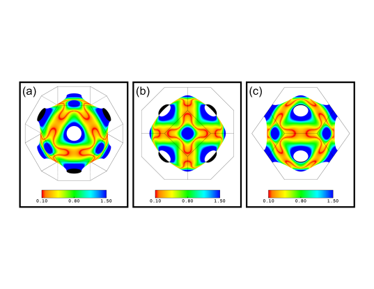
Figure 1: Fermi surface of Copper represented along three directions: (111) is shown in (a), (001) in (b) and (110) in (c). The inverse mass tensor corresponding to the denominator of eq. (19) is represented by the color in units of the inverse electron mass. Small values represented in red lead to high intensities of the charge variation.

The Cu Fermi surface is rather spherical apart from the band gaps in the $L$-directions; flat areas with strongly reduced curvature are present in the (110) directions enclosed by the two (111)-necks and two elevations in the (001) directions (see Fig. 1). These flat regions are represented along the three directions (111), (001) and (110) in red in Fig 1. The colour scale on the Fermi surface represent the strength of the inverse mass tensor (denominator of eq. (19)) which measures the flatness. This explains the anisotropic charge ripples observed experimentally and calculated from first-principles weismann . Interestingly, along the (111) direction, the neck of the Fermi surface defines a forbidden region where no electrons can scatter explaining the flat region in the charge density changes at the center of Fig. 2(a) and Fig. 2(b). The latter figures are different since they are produced by an impurity buried at different distances from the surface: in (a) it is at 6 layers below the surface while in (b) it sits much closer to the surface at the $3^{rd}$ layer under the surface. It is interesting to note that when the atom is closer to the surface, the anisotropy of the oscillations seems to loose in intensity which is induced by the stronger scattering of the surface state electrons present on the (111) surface of copper. Those surface state electrons are associated with a nearly isotropic two-dimensional circular Fermi surface. In Fig. 2(c), parts of the Fermi surface along the (001) direction (see Fig. 1(b)) is probed. This is perfomed by assuming a buried impurity in a Cu(001) sample. To improve the visualization of the curvature change observed on the Fermi surface of copper, the Fermi surface is colored with blue and green in Fig. 4(c). Here, the two regions with opposite curvatures are obvious and are sepated by a region with a low curvature that induces the focusing effect.

Figure 2: (a) and (b): Impurity induced charge density around $E_{F}$ at a height of $\approx$ 6.1 Å above the Cu(111) surface with an Co impurity sitting in the 6^th layer (a) and in the 3^rd layer (b) below the surface; (c): The case of an impurity buried at 8 layers below a Cu(001) surface is shown. Red/blue color means enhancement/reduction of the local density of states at $E_{F}$.

Multiple critical points. While the formula (18) and (19) are valid for an arbitrary number of critical points, we have analyzed in the last section only the results for one pair of critical point. If for a given $\vec{R}$-value there exist more critical points ($\vec{k}_{1},\vec{k}_{2},...$) on the Fermi surface with group velocities $\vec{v}_{1},\vec{v}_{2},...$ parallel to $\vec{R}$, than the Green function at $E_{F}$ as well as the charge density $\Delta n(\vec{r};E_{F})$ exhibit several oscillation periods as a function of R. For instance, for two points $\vec{k}_{1}$ and $\vec{k}_{2}$ with $\vec{v}_{1}$ and $\vec{v}_{2}$ parallel to $\vec{R}$, there are oscillation periods determined by the projections $k_{z1}$ and $k_{z2}$ on the direction of $\vec{R}$(see Fig. 3d). Due to the double sum over $j$, $j^{\prime}$ in (19) and (20) the charge densities $\Delta n(\vec{r};E)$ and $\Delta n(\vec{r})$ than show three periods being determined by the $k_{z}$-values $2k_{z1}$, $2k_{z2}$ and $k_{z1}+k_{z2}$. The amplitude of these oscillations are determined by the curvatures at these $k$-points as well as the wavefunctions $\Psi_{\vec{k}_{j}}(\vec{r})$ and the $t$-matrix elements $t_{\vec{k}_{j}\vec{k}_{j^{\prime}}}(E)$. It is easy to show that for $N$ critical points the number of periods is $\frac{N(N+1)}{2}$. Sometimes, e.g. for symmetry reasons, some of these periods can be the same, e.g. $\vec{k}_{1}$ and $\vec{k}_{2}$ can be different, but might have the same z-component, so that only one period $k_{z1}=k_{z2}$ exists.

The behavior is illustrated in Fig. 3 for two Fermi surface sections. Fig. 3(a) shows an ellipsoidal Fermi surface, which for each given $\vec{R}$ vector has only one pair of critical point $\vec{k}$ with group velocity $\vec{v}//\vec{R}$. Also the two vectors $\vec{k}_{j}$ and $\vec{k}_{j^{\prime}}=-\vec{k}_{j}$ are shown, the projection of which on the direction $\vec{R}$ gives the diameter of the Fermi surface (thick line) which determines the oscillation period along the direction $\vec{R}$.

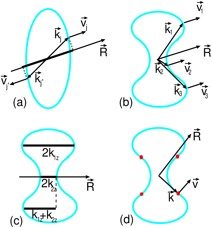
Figure 3: Examples of Fermi contours for illustrative purposes. (a) show an ellipsoidal Fermi surface, which for a given $\vec{R}$ has one critical point with a group velocity $\vec{v}$ parallel to $\vec{R}$. In (a) is shown a thick line which length defines the oscillation period. The Fermi surface sections (b), (c) and (d) are similar to the “dog’s bone” of copper Fermi surface. For an oblique orientation of $\vec{R}$ with respect to the contour’s long axis represented in (b), several critical points contribute to the oscillatory behavior. In (c), however, $\vec{R}$ is parallel to the short axis, which reduces the number of critical points. In (d), red disques show possible inflection points corresponding to higher order critical points discussed in the text. One possible direction of $\vec{R}$ probing this region is shown.

Fig. 3(b)-(d) show a more complicated Fermi surface, resembling the “dog bone” of the Cu Fermi surface. For the direction $\vec{R}$ shown in Fig. 3(b), three different $\vec{k}_{j}$ points with $\vec{v}_{j}\parallel\vec{R}$ exists, leading to a total of 6 different periods ($2k_{1z},2k_{2z},2k_{3z},k_{1z}+k_{2z},k_{1z}+k_{3z},k_{2z}+k_{3z}$) for the charge density. On the other hand, if $\vec{R}$ is perpendicular to the main axis as in Fig. 3(c), then $\vec{k_{z1}}=\vec{k_{z3}}$ and only three periods exist (indicated by the thick lines) while if $\vec{R}$ points along the main axis, there is only one solution. Thus for a given Fermi surface the situation can be quite complex.

Higher order critical points. If one of the second derivatives $\frac{\partial^{2}E}{\partial k_{x}^{2}}$ or $\frac{\partial^{2}E}{\partial k_{y}^{2}}$ in eq. 19 or 20, 22 vanishes, than the Green function expression and the charge density diverge, meaning that asymptotically these quantities decrease even with a smaller exponent than $\frac{1}{R}$, $\frac{1}{R^{2}}$ and $\frac{1}{R^{3}}$ respectively. We consider here four such cases, dropping $j$ as index of of $k_{j}$ and $t_{j}$:

a)$\frac{\partial^{2}E}{\partial k_{x}^{2}}=0$, but $\frac{\partial^{2}E}{\partial k_{y}^{2}}\neq 0$. In this case, we expand the phase factor of eq. 14 for $\Delta k_{x}$ up to $(\Delta k_{x})^{3}$:

$$\phi(\vec{k}+\Delta{\vec{k}},t+\Delta t) = kR-\frac{1}{6}\frac{t}{\hbar}\frac{\partial^{3}E}{\partial k_{x}^{3}}\Delta k_{x}^{3}-\frac{1}{2}\frac{t}{\hbar}\frac{\partial^{2}E}{\partial k_{y}^{2}}\Delta k_{y}^{2}--\frac{1}{\hbar}v\Delta k_{z}\Delta t\quad.$$ (23)

The integration over $\Delta k_{x}$, $\Delta k_{y}$, and $\Delta k_{z}$, as well as the $t$-integration can then be performed, leading to a Green function:

$$G(\vec{r}+\vec{R},\vec{r}_{1};E_{F})\sim\frac{1}{(R|\frac{\partial^{3}E}{\partial k_{x}^{3}}|)^{\frac{1}{3}}}\frac{1}{(R|\frac{\partial^{2}E}{\partial k_{y}^{2}}|)^{\frac{1}{2}}}\sim\frac{1}{R^{\frac{5}{6}}}$$ (24)

Thus the decay for larger distances is slightly slower than $\frac{1}{R}$. The charge density at $E_{F}$, $\Delta n(\vec{r}+\vec{R};E_{F})$ varies then as $\frac{1}{R^{\frac{5}{3}}}$ (instead of $\frac{1}{R^{2}}$), while the total charge $\Delta n(\vec{r}+\vec{R})$ varies as $\frac{1}{R^{\frac{8}{3}}}$ instead of the familiar $\frac{1}{R^{3}}$ of typical Friedel oscillations. For the case of copper, we observe such a situation as shown in Fig. 4(a) and (b): Here the color scale on the Fermi surface represents the inverse masse tensors strength along the $x$ and $y$ directions that are defined as diagonal elements of the inverse mass tensor of eq. 18. The directions x and y are chosen this way that $\frac{\partial^{2}E}{\partial k_{x}^{2}}$ is always larger than the y-component. It is interesting to note that in Fig. 4(a), $\frac{\partial^{2}E}{\partial k_{x}^{2}}$ is always positive for Cu, whereas $\frac{\partial^{2}E}{\partial k_{y}^{2}}$ shown in Fig. 4(b) changes sign and is equal to zero on the green line. The case considered here corresponds to the border line between the green and blue areas in fig. 4(c) where one of the second derivatives changes sign.

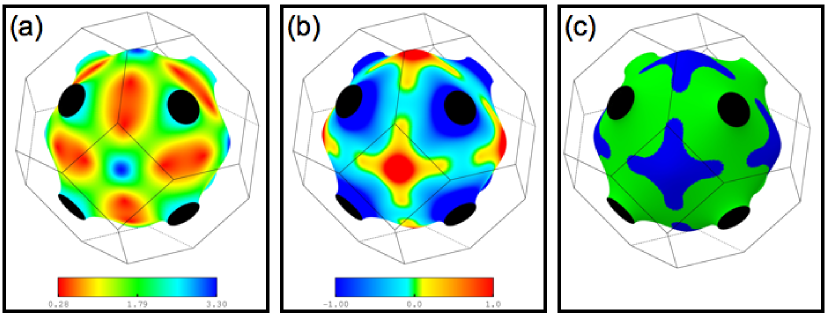
Figure 4: Fermi surface of Copper showing the diagonal elements of the inverse mass tensor in x and y direction in (a) and (b), respectively. In panel (c) the Fermi surface of copper is colored following the curvature of the Cu-Fermi surface, which determines the amplitude and the phase of the oscillations in eq. 18 and eq. 20. Blue indicates an inward curvature like the curvature of an ellipsoid, green means an outward curvature. At the boundary line between the green and blue areas the Gaussian curvature vanishes, indicating higher order critical behaviour as in Eq. 24.

b) In case that $\frac{\partial^{2}E}{\partial k_{x}^{2}}=\frac{\partial^{2}E}{\partial k_{y}^{2}}=0$, the charge density decreases again slower. Assuming that the third order derivatives have radial symmetry, the difference of the Green function varies proportional to $\frac{1}{R^{\frac{2}{3}}}$, $\Delta n(\vec{R};E_{F})$ decays as $\frac{1}{R^{\frac{4}{3}}}$, and the total charge density change drops as $\frac{1}{R^{\frac{7}{3}}}$. Such a case could be induced by the inflection points represented as a red disk spot in Fig. 3(d).

c) We consider now a case where the energy $E(k_{x},k_{y})$ is constant along a $k_{y}$-line of length $l$ perpendicular to $\vec{R}$, with constant group velocity pointing along $\vec{R}$. Then $\Delta G\propto\frac{1}{\big{(}R\big{|}\frac{\partial^{2}E}{\partial k_{x}^{2}}\big{|}\big{)}^{\frac{1}{2}}}\cdot l$ and $\Delta n(\vec{R};E_{F})\propto\frac{l^{2}}{R}$, $\Delta n(\vec{R})\propto\frac{l^{2}}{R^{2}}$.

The decrease corresponds exactly to Friedel oscillations in two dimensions ($x$ and $z$), the third dimension $k_{y}$ gives just a constant factor $l$, respectively $l^{2}$ for the charge density. Thus the decrease is very slow.

d) Finally, we consider an extreme case, that $E(k_{x},k_{y})$ is constant on a whole plane with edge length $l$ representing a perfectly flat part of the Fermi surface. Then the $k_{x}$ and $k_{y}$ integrations give just a factor of $l$ each, such that $\overset{\circ}{G}\,\!\propto l^{2}$ and $\Delta n(\vec{R};E_{F})\propto l^{4}$ and $\Delta n(\vec{R})\propto\frac{l^{4}}{R}$. Thus the Green function $\Delta G$ and the charge density have a purely oscillatory behavior with no decrease in R, while the Friedel oscillations decrease only as $\frac{1}{R}$. This behavior is typical for a one dimensional system, and represents the slowest possible decrease. Most important is that the amplitude varies with fourth power of the length $l$. Thus planar pieces of the Fermi surface lead to particular slowly decreasing oscillations, and this effect increases strongly with the size of the platelet.

Role of the surface. Here we would like to comment on the role of the surface. Up to now we have assumed a bulk system. However, as mentioned previously, the quantity of interest for the interpretation of STM experiments is the LDOS inside the vacuum at a certain distance $z$ from the surface. According to the theory of Tersoff and Harmanntersoff this distance corresponds to a position in the center of the STM tip so that tunneling parameters (bias Voltage, setpoint current) as well as the tip radius have an impact on $z$. There are different ways to implement the surface into the model. For simplicity, we will work with the spectral representation of the host Green function $\overset{\circ}{G}\,\!$ from eq. (4).

The tunneling current has contributions of multiple states, which decay differently into the vacuum. If we assume full translational invariance parallel to the surface, the parallel component of wave vector $k_{\parallel}$ is conserved. Inside the vacuum the electrons obey the Schrödinger equation of a free-electron:

$$\frac{\hbar^{2}}{2m}(k_{\parallel}^{2}-\kappa^{2})=\Delta E-\Phi$$ (25)

Here $\Phi$ is the work function of the material and $\Delta E=E-\mu$ the electron energy with respect to the chemical potential. From this a $k_{\parallel}$-dependent decay constant $\kappa$ can be derived:

$$\kappa(k_{\parallel})=\sqrt{\frac{2m}{\hbar^{2}}(\Phi-\Delta E)+k_{\parallel}^{2}}$$ (26)

The above expression shows that states with high $k_{\parallel}$-values have a higher $\kappa$ and therefore decay faster into the vacuum. Consequently the STM is more sensitive to states near the center of the surface Brillouin-zone with small $k_{\parallel}$, while short-wavelength contributions to the LDOS oscillations, corresponding to large $k_{\parallel}$, are suppressed.

In the vacuum, the wave-function of state $\Psi_{\vec{k}}$ is then:

$$\Psi(\vec{r_{\parallel}},z)\propto\exp{\left(i\vec{k}_{\parallel}\vec{r_{\parallel}}\right)}\cdot\exp{\left(-z\sqrt{\vec{k}_{\parallel}^{2}+\kappa_{0}^{2}}\right)}\quad,$$ (27)

where we defined $\kappa_{0}\equiv\kappa(k_{\parallel}=0)=\sqrt{2m(\Phi-\Delta E)}/\hbar$. In order to get an idea how this effect influences the observed patterns we perform a Taylor approximation of eq. 27 up to first order in $k_{\parallel}^{2}$:

$$\sqrt{k_{\parallel}^{2}+\kappa_{0}^{2}}\approx\kappa_{0}+\frac{k_{\parallel}^{2}}{2\kappa_{0}}\quad.$$ (28)

This approximation is valid for $k_{\parallel}\ll\kappa_{0}$. For the case of copper this is a good treatment of states having $k_{\parallel}<1.1\AA^{-1}$ while states having higher $k_{\parallel}$ values are over-suppressed . Inserting 28 in 27 gives a simple expression:

$$\exp{(-\kappa z)}\approx\exp{(-\kappa_{0}z)}\cdot\exp{\left(-\frac{k_{\parallel}^{2}z}{2\kappa_{0}}\right)}\quad.$$ (29)

This is, apart from a general attenuation of the wave functions amplitude by $\exp{(-\kappa_{0}z)}$, a Gaussian with a width of $\sigma_{k}^{2}=\kappa_{0}/z$. This implies that one can relate the wave functions from a smaller distance $z_{1}$ to greater distances $z_{2}$ by a convolution (symbol $\ast$) with a Gaussian of width $\sigma_{z}^{2}=\kappa_{0}/(z_{2}-z_{1})$:

$$\Psi(\vec{r}_{\parallel},z_{2})=\exp{\left(-\kappa_{0}(z_{2}-z_{1})\right)}\cdot\Psi(\vec{r}_{\parallel},z_{1})\ast\exp{\left(-\frac{\vec{k}_{\parallel}^{2}}{2\sigma_{z}^{2}}\right)}\quad.$$ (30)

This is a very helpful expression as the effect of the tip-sample distance $z$ can be described by a simple Gaussian filtering. If we increase $z$ either by choosing tunneling conditions, where the tip is at a larger distance from the surface or by using a blunter tip, the wave functions probed by the tip will be increasingly smeared out. If the approximation in eq. 29 is not valid, the convolution has to be performed by a Fourier transform of the last term in eq. 27, but the whole effect can still be understood as a kind of smoothing filter. This convolution can also be applied to any superposition of wave functions as well as to the Green functions which would then decay similarly.

In other words, one has to be carefull since additionally to the host Fermi surface the vacuum tunneling modifies and preselect interferences. Interferences created in the bulk can be different from those measured with the STM above the surface of the material.

Conclusion. To conclude, as the Fermi-surfaces of most materials deviate strongly from a spherical shape, the corresponding propagation of electrons is anisotropic and could reveal new effects in different materials present in nature. For instance, the combination of buried impurities and a scanning tunneling microscope could be used as a nanosonar to investigate the interior of materials. We developed and presented a theory behind the focusing effect of electronic wave oscillations. Additionally, the effect of different kind of Fermi contours’ critical points are discussed and the consequences for the decay of charge density oscillations are highlighted.

I Acknowledgements

This work was supported by the ESF EUROCORES Programme SONS under contract N. ERAS-CT-2003-980409, the Deutsche Forschungsgemeinschaft Priority Programme SPP1153 and the Deutsche Forschungsgemeinschaft Collaborative Research Centre SFB602. S.L. gratefully acknowledges support by the Alexander von Humboldt Foundation through the Feodor Lynen Program and wishes to thank D. L. Mills for discussions and hospitality.

References

(1) F. Silly, M. Pivetta, M. Ternes, F. Patthey, J.P. Pelz and W.-D. Schneider, Phys. Rev. Lett. 92, 016101 (2004).
(2)M. F. Crommie, C. P. Lutz, D. M. Eigler, Science 262, 218 (1993).
(3)V. S. Stepanyuk, L. Niebergall, W. Hergert, and P. Bruno, Phys. Rev. Lett. 94, 187201 (2005).
(4)B. Lazarovits, B. Ujfalussy, L. Szunyogh, B. L. Györffy, and P. Weinberger, J. Phys.: Condens. Matter 17 S1037 (2005).
(5)Christopher R. Moon, L. S. Mattos, B. K. Foster, G. Zeltzer, H. C. Manoharan,
Nature Nanotechnology 4, 167 (2009).
(6)F. Meier, L. Zhou, J. Wiebe, and R. Wiesendanger,
Science 320, 82 (2008).
(7)L. Zhou, J. Wiebe, S. Lounis, E. Vedmedenko, F. Meier,
S. Blügel, P. H. Dederichs, and R. Wiesendanger,
Nature Physics 6, 187 (2010).
(8) M. Schmid, W. Hebenstreit, P. Varga, and S. Crampin, Phys. Rev.
Lett. 76, 13 (1996).
(9) S. Crampin and O. R. Bryant,
Phys. Rev. B 54, 17367 (1996).
(10) P. T. Sprunger, L. Petersen,
E. W. Plummer, E. Lægsgaard, F. Besenbacher, Science 275,
1764 (1997).
(11) N. Quaas, M. Wenderoth, A. Weismann, R. Ulbrich, K. Schönhammer, Phys. Rev. B 69, 201103 (2004).
(12) O. Kurnosikov, J. H. Nietsch, M. Sicot, H. J. M. Swagten, and B. Koopmans, Phys. Rev. Lett. 102 066101 (2009).
(13) S. Heinze, R. Abt, S. Blügel, G. Gilarowski and H. Niehus, Phys. Rev. Lett. 83, 4808 (1999).
(14)A. Weismann, M. Wenderoth, S. Lounis, P. Zahn, N. Quaas, R. G. Ulbrich, P. H. Dederichs, and S. Blügel, Science 323, 1190 (2009).
(15) A. J. Heinrich, Science 323, 1178 (2009).
(16)
S. Lounis, P. Zahn, P. H. Dederichs, S. Bl ugel,
“Real Space Imaging of Fermi Surface by Scanning Tunneling Microscopy”,
European Conference on Surface Science (ECOSS24), Paris, 2006;
A.Weismann, M. Wenderoth, N. Quaas, and R. G. Ulbrich
Electron scattering at subsurface impurities in noble metals at 8K
Invited talk at ICSS-12 /Nano-8 Venice (2004).
(18)A. Weismann, PhD thesis, Georg-August-Universität zu Göttingen, 2008.
(19)O. Brovko, V. Stepanyuk, W. Hergert, and P. Bruno,
Phys. Rev. B 79, 245417 (2009).
(20)Ye. Avotina, Yu. Kolesnichenko, and J. van Ruitenbeek,
Phys. Rev. B 80, 115333 (2009);
Ye. S. Avotina, Yu. A. Kolesnichenko, A. N. Omelyanchouk, A. F. Otte,
and J. M. van Ruitenbeek, Phys. Rev. B 71, 115430 (2005).
(21) F. J. Garcia-Vidal, P. L. de Andres, and
F. Flores, Phys. Rev. Lett. 76, 807 (1996).
(22) K. Reuter, P. L. Andres, F. J. Garcia-Vidal, D. Sestovic,
F. Flores, K. Heinz, Phys. Rev. B 58, 14036 (1998).
(23) L. M. Roth, H. J. Zeiger, T. A. Kaplan,
Phys. Rev. 149, 519 (1966).
(24)M. A. Ruderman, C. Kittel, Phys. Rev. 96, 99 (1954); T. Kasuya, Prog. Theor. Phys. 16, 45 (1956);K. Yosida,
Phys. Rev. 106, 893 (1957).
(25) P. Grünberg, R. Schreiber, Y. Pang,
M. B. Brodsky, and H. Sower, Phys. Rev. Lett. 57, 2442 (1986).
(26) S. S. P. Parkin, N. More, and K. P. Roche, Phys. Rev. Lett.
64, 2304 (1990).
(27) P. Bruno, C. Chappert, Phys. Rev. Lett. 67, 1602 (1991).
(28) J. Tersoff, D. R. Hamann, Phys. Rev. Lett. 50, 1998 (1983).
(29) N. Papanikolaou, R. Zeller and P. H. Dederichs,
J. Phys.: Condens. Matter 14, 2799 (2002)