The Emergence of El-Niño as an Autonomous Component in the Climate Network

Abstract

We construct and analyze a climate network which represents the interdependent structure of the climate in different geographical zones and find that the network responds in a unique way to El-Niño events. Analyzing the dynamics of the climate network shows that when El-Niño events begin, the El-Niño basin partially loses its influence on its surroundings. After typically three months, this influence is restored while the basin loses almost all dependence on its surroundings and becomes autonomous. The formation of an autonomous basin is the missing link to understand the seemingly contradicting phenomena of the afore–noticed weakening of the interdependencies in the climate network during El-Niño and the known impact of the anomalies inside the El-Niño basin on the global climate system.

It was recently suggested that climate fields such as temperature and geopotential height at a certain pressure level can be represented as a climate network Tsonis et al. (2006). In this network, different regions of the world are represented as nodes which communicate by exchanging heat, material, and by direct forces. These interactions are represented by the links of the climate network. Interactions between two nodes may also exist due to processes which take place outside the atmospheric pressure level or through interactions with the ocean and the lands. Each link is quantified by a weight based on measures of similarity between the time series (e.g. correlations) of the corresponding individual nodes (see Castrejòn-Pita and Read (2010) for an experimental evidence for the relations between heat exchange and synchronized fluctuations of the temperature field).

Recent studies Yamasaki et al. (2008); Tsonis and Swanson (2008); Gozolchiani et al. (2008) show that many links in the climate network break during El-Niño events. The climate network contains several types of links, that have different levels of responsiveness to El-Niño. From the maps of Tsonis and Swanson Tsonis and Swanson (2008), one can locate the responsive nodes (the nodes attached to the most responsive links) to be in the pacific El-Niño Basin (ENB) Bjerknes (1969). These maps together with the tremendous impact of the El-Niño Southern Oscillations on world climate, suggest that ENB have a unique dynamical role in the dynamics of the climate network. Indeed ENB has unique topological properties. Its connectivity and clustering coefficient fields studied by Donges et. al. Donges et al. (2009a) can be distinguished from their surrounding by their particularly higher values. Also, the betweenness centrality field Donges et al. (2009b) in ENB is very low. However, the dynamics related to the interaction of ENB with its surroundings and the origin of its unique features are still not known Storch and Zwiers (2003).

In this Letter we follow the dynamics of the climate network in time, between the years 1979 and 2009 where eight El-Niño events took place. We identify a cluster around ENB that shows a clear autonomous behavior during El-Niño epochs, and determine the dynamics of its interactions with the surroundings. We also find an epoch of a decreased influence of ENB on the surroundings, typically three months before the emergence of the autonomous behavior. Our findings resolve the seemingly contradictory situation of decreased interactions of ENB with its surroundings on one hand, as explored in previous works Yamasaki et al. (2008); Tsonis and Swanson (2008); Gozolchiani et al. (2008), and the known influence of ENB on world climate on the other hand. We find that only the influence of the surroundings on the ENB region is significantly reduced, creating, apparently, a dynamical autonomous source within this region which influences its surroundings.

The adjacency matrix in our climate network analysis is based on a similarity measure between time series of temperatures (after removal of the annual trend) at the pressure level of 1000mb covering the last 30 years. In the current work we pick 726 nodes from the Reanalysis II grid noa , such that the globe is covered approximately homogeneously. The similarity measure $W_{l,r}^{y}$ we use is defined as follows. First we identify the value of the highest peak of the absolute value of the cross covariance function. Then we subtract the mean of the cross covariance function and divide the difference by its standard deviation (see  Yamasaki et al. (2008); Gozolchiani et al. (2008) for further details). The indices $l$ and $r$ represent two nodes, and $y$ is the beginning date of a snapshot of the network, measured over 365 days with extended period of 200 days of shifts needed for evaluating the cross covariance. The time shift of the highest peak of the cross covariance function from zero time shift is denoted $\theta^{y}_{l,r}$. The sign of $\theta^{y}_{l,r}$ stands for the dynamical ordering of $l$ and $r$ (and hence $\theta^{y}_{l,r}=-\theta^{y}_{r,l}$). In directed graph theory terms, when $\theta^{y}_{l,r}>0$ the link is regarded as outgoing from node $l$ and incoming to node $r$. Until now, such ordering or direction were not considered for constructing climate networks. Our method, thus, enables to distinguish between in– and out– links.

The adjacency matrix of a weighted directed climate network is defined :

$$A^{y}_{l,r}=\left(1-\delta_{l,r}\right)\Theta\left(\theta^{y}_{l,r}\right)W^{y}_{l,r}$$ (1)

whereas $\Theta(x)$ is the Heaviside function.

The in– and out– weighted degrees are defined :

$$I^{y}_{l}=\sum_{r}A^{y}_{r,l}$$ (2a)

$$O^{y}_{l}=\sum_{r}A^{y}_{l,r}$$ (2b)

The $I$ and $O$ fields represent the level of the dependence of a node on its surrounding, and the level of its influence on the surrounding, respectively.

The total weighted degree (also denoted “vertex strength” Barrat et al. (2004)) of a node $l$ is defined as :

$$D^{y}_{l}=\sum_{r}\left(1-\delta_{\theta_{l,r},0}\right)(A^{y}_{l,r}+A^{y}_{r,l})+\sum_{r}\delta_{\theta_{l,r},0}A^{y}_{l,r}$$ (3)

Fig. 1a shows the time dependence of $D$ for each node in the network. Two main observations can be clearly seen from this figure. First, weighted degrees of the nodes yield an extremely persistent quantity fn (1), and different geographical regions have typical values over time. A second notable pattern is the horizontal bright stripes that appear during El-Niño events. The second feature further supports the finding Yamasaki et al. (2008); Tsonis and Swanson (2008); Gozolchiani et al. (2008) that many links of the climate network break during El-Niño events.

Inside the mid range of node indices, between 300 and 500, there is a group of nodes, ${\bf C}$, that have lower values at any time, and are specifically distinct during El-Niño (Fig. 1a). These low values and their distinct response to El-Niño, as we will explicitly show, are mainly due to in– links. When studying the in– and out– links separately, we find that the spatial distribution of the in– weighted degrees $I_{l}^{y}$ is much broader compared to the distribution of the out– weighted degrees $O_{l}^{y}$, at any time $y$, typically by 10 to 20 percent. The 90-th percentile (statistics is collected over time) yields a deviation of 30 percents. As shown below, this difference between $I$ and $O$ is mainly contributed by the group ${\bf C}$ discussed above. In order to follow the different dynamical behavior of $I$ and $O$, we apply the following approach.

We consider only links that are related directly to the El-Niño dynamics by focusing on the group of nodes ${\bf C}$ that have extremely low weighted degrees during El-Niño events:

$${\bf C}\equiv\left\{l\ |\ \left<D^{y}_{l}\right>_{y\in EN}\leq T\right\}$$ (4)

where $T=2150$ is a threshold fn (2), and the triangular brackets stand for averaging over all El-Niño events. The group ${\bf C}$ which includes 14 nodes is part of ENB, and is notably located in the eastern equatorial part of ENB, which is known to have a large scale upwelling of cold ocean water, yielding a “cold tongue” Bjerknes (1969) which deforms during El-Niño (see Fig. 6a for its location).

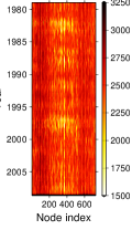
(a) $D$–field

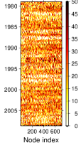
(b) $I$–field

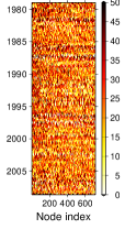
(c) $O$–field

Figure 1: Weighted degrees as a function of time (y axis) and the node index (x axis). (a) Total weighted degree $D^{y}_{l}$. (b) The microscopic contributions to the weighted incoming degree of ${\bf C}$, $I^{y}_{\bf C}$. (c) The microscopic contributions to the weighted outgoing degrees, $O^{y}_{\bf C}$. One should bare in mind that each point is compiled from records of 565 days : 365 days + 200 days of shifts. The representative point in all figures for each 565 period is the beginning date of the period

We find that measuring the dynamics of the interactions of the ${\bf C}$ region with its surroundings yields a sensitive tool to quantify the responses of $I$ and $O$ to El-Niño events. One can define $I^{y}_{\bf C}$ and $O^{y}_{\bf C}$, the in– and out– weighted degree of ${\bf C}$, respectively, in the same manner we defined the weighted degrees for nodes. We consider only links between pairs of nodes where one node belongs to ${\bf C}$ and the other does not. Fig. 2 shows the time dependence of these two variables. As seen in the figure, the responses of the in– and out– degrees to El-Niño seem to be anti-correlated. When the in–degree drops, the out–degree slightly increases. The interpretation is that the nodes inside ${\bf C}$ lose large part of their dependence on the surrounding, while slightly increase their influence outside, thus becoming significantly more autonomous during El-Niño. Note that the excess of out– links over in– links is evident also in normal times. The detailed space-dependent picture, however, is even richer, as discussed below.

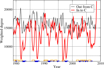
Figure 2: Plot of the weighted in– and out– degrees of ${\bf C}$, $I^{y}_{\bf C}$ and $O^{y}_{\bf C}$, respectively. The blue marker along the x–axis shows the periods in which the NINO3.4 (see e.g. nin ) mean temperature exceeds $0.4^{o}C$, which is one of the criterions indicating an El-Niño event. The orange markers show the extended periods in which our analysis is influenced by the events because of the 365 days integration of the cross covariance function.

The spatial dependence of $I^{y}_{\bf C}$ and $O^{y}_{\bf C}$ is explored by what we call the “microscopic” contributions from each one of the 712 nodes that do not belong to ${\bf C}$. These microscopic contributions can be visualized (Figs. 1LABEL:sub@fig:in_clust,LABEL:sub@fig:out_clust) as they evolve in time.

El-Niño events influence $I$ and $O$ in a very different way, having a rather peculiar phase locking. Strong El-Niño events weaken the links, yielding smaller microscopic contributions to both $I^{y}_{\bf C}$ and $O^{y}_{\bf C}$ (white horizontal stripes in Figs. 1LABEL:sub@fig:in_clust,LABEL:sub@fig:out_clust), just like Fig. 1a. However, the in–links are significantly more vulnerable to El-Niño compared to the out–links. Moreover, before each major event of weakening $I$-field, there is a short, weaker response of weakening of the $O$-field. After the weakening epoch of both fields the $O$ field recovers, and thereafter the $I$ field recovers as well, leading to a full oscillation of both fields fn (3). It is possible to summarize the situation by saying that the ${\bf C}$ nodes lose their autonomous power at the beginning of an El-Niño event, but thereafter, during the event, it recovers and becomes significantly more autonomous than the average. Despite the prominent difference during El-Niño between their dynamics, the $I$ and $O$ fields exhibit a remarkable static mirror similarity. Both fields are found to be highly asymmetrical with respect to the equator, at all times. We find that the in– links (going into ${\bf C}$) mainly originate from the northern latitudes, while the out– links (out from ${\bf C}$) mainly target towards the southern latitudes.

In order to detect the weak response of $O^{y}_{\bf C}$, we next consider specific “microscopic” contributions that have the lowest weight values, disregarding the rest of the field. This filters out noise that is not related to the observed slight weakening. We count (Fig. 3) the number of nodes having microscopic contribution to the weighted in– and out– degrees under a weight threshold of 5, defined as $I^{*}$ and $O^{*}$ respectively. We will show (Fig. 4) that there is little sensitivity to this threshold value. Thus, a rise of $O^{*}$ (red) in Fig. 3 corresponds to nodes losing their dependence on ${\bf C}$. Shortly after such events we see a significant rise of the $I^{*}$ (black) that corresponds to nodes losing their influence on ${\bf C}$. As is clearly seen in Fig. 3, the $I^{*}$ and $O^{*}$ oscillations begin at the onset of El-Niño events.

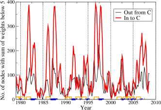
Figure 3: Number of nodes outside ${\bf C}$ having sum of weights below 5 directing towards ${\bf C}$ (in), $I^{*}$, or from ${\bf C}$ (out),$O^{*}$. The blue and orange markers are described in the previous figure

Next, we extract the time lag between the two coherent oscillations of $I^{*}$ and $O^{*}$ using the cross covariance function. In Fig. 4 we show the cross covariance between the two curves of Fig. 3, for several threshold values. The peak of the cross covariance function shows that $O$ lags after $I$ in $100\pm 50$ days fn (5). The sharp correlation between the number of “weak” nodes in both directions (in and out) as well as the time lag is persistent up to a threshold value of 15. The other peaks of the cross correlation function are related to the quasi-periodicity of the El-Niño southern oscillations.

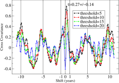
Figure 4: Cross covariance of the number of links below various thresholds going into and out from cluster ${\bf C}$ (in and out respectively, Fig. 3). In the positive direction of the x-axis, the number of in– links lags in time after the out– links.

Next we show in Figs. 5LABEL:sub@fig:indistnonen,LABEL:sub@fig:outdistnonen the spatial distribution of $I^{y}_{l}$ and $O^{y}_{l}$ during normal (non-El-Niño) times (We used the GMT tool  Wessel and Smith (1998) to overlay the fields on maps). Our statement about the in–weighted degrees having a broader distribution by 10 to 20 percent at all times, gets its direct spatial interpretation. As seen in Fig. 5, the out– weighted degree spatial field is much more homogeneous compared to the in– weighted degree which has a sharp minimum around ENB. This asymmetry between $I_{\bf C}^{y}$ and $O_{\bf C}^{y}$ becomes significantly more pronounced during El-Niño periods (see Fig. 6). The cluster ${\bf C}$ is marked explicitly with large blue circles. In this sense, ENB gets significantly more autonomous during El-Niño. A full time dependent animation of these maps is available at  prl . Note that the fields in Figs. 5 and  6 have been calculated without any correlation threshold.

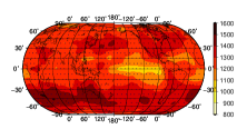
(a) $\left<I_{l}^{y}\right>_{y\not\in El-Nino}$

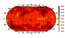
(b) $\left<O_{l}^{y}\right>_{y\not\in El-Nino}$

Figure 5: Spatial distribution of the weighted degrees of nodes (in and out) averaged over non-El-Niño times. The nodes of the network are shown by small dots.

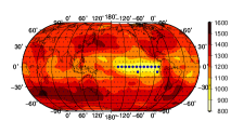
(a) $\left<I_{l}^{y}\right>_{y\in El-Nino}$

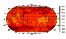
(b) $\left<O_{l}^{y}\right>_{y\in El-Nino}$

Figure 6: Spatial distribution of the weighted degrees of nodes (in and out) averaged over El-Niño times. The nodes of the network are shown by small dots. The nodes belonging to ${\bf C}$ are shown on the weighted in–degree map as larger blue circles

In summary, we have found a new dynamical pattern that reflects the coupling between the El-Niño basin, and the rest of the world. ENB becomes significantly more autonomous during El-Niño, losing a large fraction of its in–links, while still having out–links. This kind of topology is reminiscent of pacemakers in network models Timme (2006). The major impact of events inside ENB on world climate on one hand, and the weakened correlations during El-Niño episodes on the other hand Yamasaki et al. (2008); Tsonis and Swanson (2008); Gozolchiani et al. (2008), are thus not contradicting. In fact, the uni–directional interaction of ENB with large parts of the climate network might suggest the origin for its significant dynamical role in the global climate.

Our results also suggest the existence of a robust delayed relationship between the inward and outward coupling of ENB with the rest of the world. The emergence of the autonomous behavior is consistently following, after typically 3 months, a short and weak episode of a decreased outward coupling. The two fields (outward and inward coupling) oscillate with a phase shift.

We also find that ENB is forced more by the northern hemisphere than by the southern, and forces the southern hemisphere more than it forces the northern. Since the annual cycle in the two hemispheres is opposite, this north–south asymmetry might be related to the known (not yet fully understood) partial phase locking of the ENSO cycle with the annual cycle (see e.g. Jin et al. (1994); Tziperman et al. (1994)).

Acknowledgements We thank the EU EPIWORK project, the Israel Science Foundation, DTRA, ONR, and Research project for a sustainable development of economic and social structure dependent on the environment of the eastern coast of Asia.

References

- Tsonis et al. (2006) A. A. Tsonis, K. L. Swanson, and P. J. Roebber, Bull. Am. Meteorol. Soc. 87, 585 (2006).
- Castrejòn-Pita and Read (2010) A. A. Castrejòn-Pita and P. L. Read, Phys. Rev. Lett. 104, 204501 (2010).
- Yamasaki et al. (2008) K. Yamasaki, A. Gozolchiani, and S. Havlin, Phys. Rev. Lett. 100, 228501 (2008).
- Tsonis and Swanson (2008) A. A. Tsonis and K. L. Swanson, Phys. Rev. Lett. 100, 228502 (2008).
- Gozolchiani et al. (2008) A. Gozolchiani, K. Yamasaki, O. Gazit, and S. Havlin, Europhys. Lett. 83, 28005 (2008).
- Bjerknes (1969) J. Bjerknes, Monthly Weather Review 97, 163 (1969).
- Donges et al. (2009a) J. F. Donges, Y. Zou, N. Marwan, and J. Kurths, Eur. Phys. J. Special Topics 174, 157 (2009a).
- Donges et al. (2009b) J. F. Donges, Y. Zou, N. Marwan, and J. Kurths, Europhys. Lett. 87, 48007 (2009b).
- Storch and Zwiers (2003) H. V. Storch and F. W. Zwiers, Statistical analysis in climate research (Cambridge University Press, Cambridge, 2003), chap. 7, p. 131.
- (10) http://www.cdc.noaa.gov, NCEP Reanalysis data, NOAA/OAR/ESRL PSD, Boulder, Colorado, USA.
- Barrat et al. (2004) A. Barrat, M. Barthelemy, R. Pastor-Satorras, and A. Vespignani, Proc. Nat. Ac. Sc. 101, 3747 (2004).
- fn (1) The standard deviation of a weighted degree over time is typicaly between 13 and 16 percent of its mean value.
- fn (2) We chose as the highest possible value, such that zones that do not belong to ENB are not part of .
- (14) http://www.cpc.ncep.noaa.gov/products/analysis_monitoring/ensostuff/nino_regions.shtml.
- fn (3) During major events we can even see a full second oscillation in which the field recovers, and weakens again, giving rise to a second major weakening of .
- fn (5) The origin of error is due to low sampling rates since we take a snapshot of the network every 50 days.
- Wessel and Smith (1998) P. Wessel and W. H. F. Smith, EOS Trans. Amer. Geophys. U. 79, 579 (1998).
- (18) http://physionet.ph.biu.ac.il/~gozolaa/PRL_ENSOPMgozyamhav.
- Timme (2006) M. Timme, Europhys. Lett. 76(3), 367 (2006).
- Jin et al. (1994) F. F. Jin, D. Neelin, and M. Ghil, Science 264, 70 (1994).
- Tziperman et al. (1994) E. Tziperman, L. Stone, M. A. Cane, and H. Jarosh, Science 264, 72 (1994).