Surface Curvature Effects on Reflectance from Translucent Materials

Abstract

Most of the physically based techniques for rendering translucent objects use the diffusion theory of light scattering in turbid media. The widely used dipole diffusion model [JMLH01] applies the diffusion-theory formula derived for the planar surface to objects of arbitrary shapes. This paper presents first results of our investigation of how surface curvature affects the diffuse reflectance from translucent materials.

1 Introduction

Translucent materials, such as human skin, marble, wax, fruits, more scatter light than absorb it. Therefore, when a photon enters such a material, it undergoes many scattering events under the surface before it leaves the material. Such a light behavior is well described by the Bidirectional Surface Scattering Distribution Function (BSSRDF) [NRH⁺77]. Based on the light diffusion theory, Jensen et al. [JMLH01] suggested the dipole diffusion model for BSSRDF. This model applies an expression for reflectance from a turbid half-space to arbitrarily shaped objects. The multipole [DJ05, DJ06] and quadpole [DJ08] models have been suggested to describe more complicated geometries - a multilayered slab (or half-space) and a right-angle corner, respectively. Jensen et al. [DJ08] showed that a big variety of shapes can be rendered by combining photon tracing and a scheme for interpolating between dipole and quadpole and between quadpole and multipole models wherever appropriate. However, they do not focus on how the BSSDRF itself changes as a flat surface is replaced with a curved one. It is difficult to devise how their interpolation scheme can be used with approaches that do not use photon tracing - for example, the curvature-based method [Kol07]. Our goal is to investigate how inclusion of curvature may change the diffusion BSSRDF model. A BSSRDF model that includes curvature effects could be easily incorporated into many existing approaches for rendering translucent materials. We present here preliminary results of our study.

2 Diffusion Equation

Under the assumption that light scattering in a turbid medium dominates absorption, light transport in it is well described with the diffusion theory [Far92]. The fluence rate $\Psi(\mathbf{r})$ obeys the modified Helmholtz equation [Far92]

$$\Delta\Psi-\sigma_{tr}^{2}\Psi=-D^{-1}\delta(\mathbf{r}-\mathbf{r}_{0})$$ (1)

where $\sigma_{tr}=\sqrt{3\sigma_{a}(\sigma_{s}^{\prime}+\sigma_{a})}$ is the effective transport coefficient, $\sigma_{s}^{\prime}$ is the reduced scattering coefficient, $\sigma_{a}$ is the absorption coefficient, $D=\frac{1}{3(\sigma_{s}^{\prime}+\sigma_{a})}$ is the diffusion coefficient. We refer the reader to [JMLH01, Far92] for explanation of the physical meaning of the quanitities. In the above equation, we assume that there is a single source in the medium, and it is located at a point $\mathbf{r}_{0}$.

Let us first consider the case of translucent material occupying the half-space $z>0$. The point source is at $\mathbf{r}_{0}=(0,0,z_{0})$. Farrell et al. [Far92] showed that quite an accurate solution can be obtained by using the boundary condition $\Psi|_{z=-z_{b}}=0$ and putting the image source at the point $\mathbf{r}_{0}=(0,0,-z_{0}-2z_{b})$, where $z_{b}=2AD$, and $A$ is calculated as described in [JMLH01, Far92]. The resulting fluence is

$$\Psi(\rho,z_{0})=\frac{1}{4\pi D}\left(\frac{e^{-\sigma_{tr}r_{1}}}{r_{1}}+\frac{e^{-\sigma_{tr}r_{2}}}{r_{2}}\right),$$

where $r_{1}$ and $r_{2}$ are the distances to the source and image source, respectively; that is,

$$r_{1} = [(z-z_{0})^{2}+\rho^{2}]^{1/2}$$ (2)

$$r_{2} = [(z+z_{0}+2z_{b})^{2}+\rho^{2}]^{1/2}$$ (3)

The reflectance is calculated from the fluence using the formula

$$R=-D\nabla\Psi$$ (4)

where the gradient is evaluated at the interface. In the planar case, this gives

$$R(\rho,z_{0}) = \frac{1}{4\pi}\left[z_{0}(\sigma_{tr}+\frac{1}{r_{1}})\frac{e^{-\sigma_{tr}r_{1}}}{r_{1}^{2}}+\right.$$ (5)

$$\left.+(z_{0}+2z_{b})(\sigma_{tr}+\frac{1}{r_{2}^{2}})\frac{e^{-\sigma_{tr}r_{2}}}{r_{2}^{2}}\right]$$

where $r_{1}$ and $r_{2}$ are calculated for $z=0$.

The dipole diffusion model [JMLH01] applies the above formula to an arbitrary shaped air-material interface by calculating $r_{1}$ and $r_{2}$ as the distance from a point being shaded to the source and image source, respectively.

3 Exact Solution for a Sphere

Suppose the turbid medium is confined within a sphere having the radius $R_{0}$ and the center at $z=R_{0}$. In addition to Cartesian coordinates, we will also use the polar system of coordinates with $r$ counted from the sphere center and $\theta$counted from the $z$ axis. We assume that $R_{0}$is much bigger than the mean free path for photons scattered in the medium, we can use the same boundary condition as in the planar case - namely, the fluence rate vanishes at a distance of $z_{b}$ from the sphere surface. In other words, $\Psi$ is zero at a sphere of the radius $R=R_{0}+z_{b}$. We will solve eq. (9) with the boundary condition $\Psi|_{r=R}=0$ following the method described in [Mat71]. The solution of the modified Helmholtz equation 9with the zero boundary condition on the sphere $r=R$ can be written as

$$\Psi(r,\theta)=\begin{cases}\sum_{m=0}^{\infty}A_{m}\frac{I_{m+1/2}(\sigma_{tr}r)}{\sqrt{r}}P_{m}(\cos\theta)\mbox{ , }r<r^{\prime}\\ \sum_{m=0}^{\infty}B_{m}\frac{1}{\sqrt{r}}[I_{m+1/2}(\sigma_{tr}r)\times\\ \times K_{m+1/2}(\sigma_{tr}R)-K_{m+1/2}(\sigma_{tr}r)\times\\ \times I(\sigma_{tr}R)]P_{m}(\cos\theta)\mbox{ , }r>r^{\prime}\end{cases}$$ (6)

where $r^{\prime}$ is the distance of the point source from the sphere center; that is, we suppose that$\mathbf{r}_{0}$ has the polar coordinates $r=r^{\prime}$ and $\theta=0$. The functions $I_{v}(r)$ and $K_{\nu}(r)$ are the modified Bessel functions [MA70]. The constants $A_{m}$and $B_{m}$ are determined by stitching the solutions 6 at the sphere $r=r^{\prime}$. The function $\Psi$ is continuous, but its derivative is not. In a manner similar to that used in [Mat71], we integrate eq. 9 over an infinitisemally thin region confined by parts of spherical surfaces with radiuses $r=r^{\prime}+\epsilon$ and $r=r^{\prime}-\epsilon$ and containing the point$\mathbf{r}_{0}$. We utilize the Gauss theorem and get

$$\left(\frac{\partial\Psi}{\partial r}\Big{|}_{r^{\prime}+\epsilon}-\frac{\partial\Psi}{\partial r}\Big{|}_{r^{\prime}-\epsilon}\right)=\frac{1}{r^{\prime 2}}\delta(\Omega)$$ (7)

where $\Omega$ is the solid angle variable. The delta function $\delta(\Omega)$ can be decomposed in terms of the Legendre polynomials as [Mat71]

$$\delta(\Omega)=\sum_{m=0}^{\infty}\frac{(2m+1)}{4\pi}P_{m}(\cos\theta)$$ (8)

Substituting eq. (8) into eq. (7) and calculating the derivatives from eq. (6), we arrive at an equation for $A_{m}$and $B_{m}$. One more equation for them is obtained by requiring continuity of $\Psi$ at $r=r^{\prime}$. Solving the resulting system of two equations, we get

$$\Psi(r,\theta) = \frac{1}{4\pi D}\left[\sum_{m=0}^{\infty}\frac{(2m+1)}{\sqrt{rr^{\prime}}}I_{m+1/2}(\sigma_{tr}r^{\prime})\times\right.$$

$$\left.\times I_{m+1/2}(\sigma_{tr}r)\frac{K_{m+1/2}(\sigma_{tr}R)}{I_{m+1/2}(\sigma_{tr}R)}P_{m}(\cos\theta)-\frac{e^{-\sigma_{tr}\widetilde{r}}}{\widetilde{r}}\right]$$

where

$$\tilde{r}=(r^{2}+r^{\prime 2}-2rr^{\prime}\cos\theta)^{\nicefrac{{1}}{{2}}},$$

and we used equality 10.2.35 from [MA70].

To find the reflectance, we choose $r^{\prime}=R_{0}-z_{0}$, apply eq. 4 and set $r=R_{0}$ and get

$$R(r,\theta) = \frac{1}{4\pi}\sigma_{tr}\left\{\sum_{m=0}^{\infty}\frac{(2m+1)}{\sqrt{R_{0}r^{\prime}}}I_{m+1/2}(\sigma_{tr}r^{\prime})\times\right.$$

$$\times I^{\prime}_{m+1/2}(\sigma_{tr}R_{0})\frac{K_{m+1/2}(\sigma_{tr}R)}{I_{m+1/2}(\sigma_{tr}R)}P_{m}(\cos\theta)+$$

$$\left.+[z_{0}\cos\theta-R_{0}(\cos\theta-1)](\sigma_{tr}+\frac{1}{r_{1}})\frac{e^{-\sigma_{tr}r_{1}}}{r_{1}^{2}}\right\}$$

4 Results

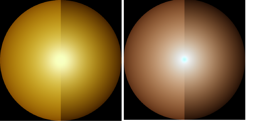
Figure 1: A spherical potato (left) and a marble sphere (right) illuminated with a stencil beam, which enters at the image center, normally to the image plane. Each of the spheres is rendered using the exact solution proposed (left part of a sphere) and the dipole diffusion model (right part of a sphere).

We calculated the reflectance from translucent spheres of various radiuses. The incident light is a pencil beam entering a sphere at $x=0,$y=0 . Ideally, we should consider a line of sources situated along the $z$ axis. But it was shown in [Far92] that they all can be replaced with a single source located $z=\nicefrac{{1}}{{(\sigma_{s}^{\prime}+\sigma_{a})}}$. The plot below shows how the reflectance depends on the distance from the point of light entrance measured along the surface (that is, the length of a geodesic connecting the entrance point and the point of interest). The calculations were done for the scattering coefficient $\sigma_{s}^{\prime}=1mm^{-1}$and absorption coefficient $\sigma_{a}=0.01mm^{-1}$ (note that in [Far92], the same quantities are designated as $\mu_{s}^{\prime}$ and $\mu_{a}$, respectively). These values of the scattering and absorption coefficients are typical for human tissue (see [JMLH01]). It can be seen that in this case, the difference between the exactly computed reflectance and that found by the dipole diffusion model becomes noticable only when the radius approaches 1 cm.

Figure 1 above shows visualization of light reflection from spheres having a radius of 1 cm in two cases - a potato, on the left, and marble, on the right. As for the plot given below, we assume that a sphere is lit up by a stencil beam entering the sphere at the center of the image. The left part of each of the image corresponds to the exact calculation we describe above. The right part is computed using the diffuse dipole approximation. We used the measured values $\sigma_{s}^{\prime}$ and $\sigma_{a}$ reported in [JMLH01]. Because the amount of reflected light decays with distance from the entrance point very rapidly, we applied the tone mapping operator to a calculated HDR image. We chose the logarithmic mapping operator[DMAC03], as it is simple and robust, and a source code for its implementation is available on the web.

Probably, we could anticipate in advance that the diffuse dipole model would underestimate the reflectance. However, our investigation shows that this underestimation is small when curvature radiuses are of the scale of several centimeters and more for such materials as marble, potato, human tissue.

5 Future Work

The investigation presented here definitely lacks comparison of analytical results with Monte-Carlo simulations. We are working on this and plan to report them elsewhere when the work is complete. Also, we would like to consider the case of arbatrarily curved surfaces. It would be interesting to try to build a phenomenological model for reflectance from a translucent material with an arbitrary surface. It can be sought as a function of principal curvatures at the point of light entrance. An approximate solution for slightly curved surfaces (Appendix A presents an approximate solution for the modified Helmholtz equation in the case of a curved boundary) can serve as a base in attempts to construct a phenomenological model. Monte-Carlo simulations can be used for validation of such a model. A big potential of the phenomenological approach to constructing BSSRDF models has been proven by successfull development of an empirical BSSRDF model described in [DLR⁺09]. A BSSRDF model including surface curvature could be incorporated into the curvature-based method [Kol07]. It could be used for investigating perceptional effects, such as color shift at the terminator line [Gre04].

Appendix A An Approximate Solution for Slightly Curved Surfaces

We consider the modified Helmholtz equation

$$\Delta\Psi-\sigma_{tr}^{2}\Psi=-D^{-1}\delta(\mathbf{r}-\mathbf{r}_{0})$$ (9)

where $\mathbf{r}$ is a point in three-dimensional space, and $\mathbf{r}=(x,y,z)$ in the Cartesian coordinate system. The source is located at the point $\mathbf{r}_{0}=(0,0,a)$. We are searching for a solution of this equation for $z>f(x,y)$ with the boundary condition

$$\Psi|_{z=f(x,y)}=0$$

where $z=f(x,y)$ is the equation describing some surface. Let’s assume deviation of the surface from a plane to be small and introduce a small parameter, $\epsilon,$ to describe this, so that the surface equation becomes

$$z=\epsilon f(x,y),$$

Let us search a solution to the modified Helmhotz equation as a series in $\epsilon$.

$$\Psi=\Psi_{0}+\epsilon\Psi_{1}+\epsilon^{2}\Psi_{2}+...$$

Then $\Psi_{0}$ is the solution for the planar case, which is given by

$$\Psi_{0}=\frac{1}{4\pi D}\left(\frac{e^{-\sigma_{tr}r_{1}}}{r_{1}}+\frac{e^{-\sigma_{tr}r_{2}}}{r_{2}}\right),$$

where $r_{1}$ and $r_{2}$ are the distances to the source and image source, respectively; that is,

$$r_{1} = [(z-a)^{2}+x^{2}+y^{2}]^{1/2}$$ (10)

$$r_{2} = [(z+a)^{2}+x^{2}+y^{2}]^{1/2}$$ (11)

We know the Green function for the planar case, so let’s try to find the boundary condition for $\Psi_{1}$ at the plane $z=0$. It can be found by extending $\Psi_{0}$ in $z$. We know that $\Psi$ takes a zero value at the surface; therefore, we have

$$\Psi|_{z=\epsilon f(x,y)}=0=\Psi_{0}|_{z=0}+\frac{\partial\Psi_{0}}{\partial z}\Big{|}_{z=0}\epsilon f(x,y)+\epsilon\Psi_{1}|_{z=0}+...$$

Each term in the $\epsilon$ series should be equal to zero; therefore, we get

$$\Psi_{1}|_{z=0}=-\frac{\partial\Psi_{0}}{\partial z}\Big{|}_{z=0}f(x,y)$$ (12)

Therefore, $\Psi_{1}$for $z>0$ can be found as

$$\Psi_{1}(x,y,z)=\iint\frac{\partial\Psi_{0}(x^{\prime},y^{\prime},z^{\prime})}{\partial z^{\prime}}\Big{|}_{z^{\prime}=0}f(x^{\prime},y^{\prime})\frac{\partial G}{\partial z^{\prime}}\Big{|}_{z^{\prime}=0}dx^{\prime}dy^{\prime}$$ (13)

where $G$ is the Green function for the Helmholtz equation and boundary conditions of the form $\Psi|_{z=0}=\psi(x,y)$. Namely,

$$G(x,y,z,x^{\prime},y^{\prime},z^{\prime})=\frac{1}{4\pi D}\left(\frac{e^{-\sigma_{tr}r_{1}^{\prime}}}{r_{1}^{\prime}}+\frac{e^{-\sigma_{tr}r_{2}^{\prime}}}{r_{2}^{\prime}}\right),$$

where $r_{1}$ and $r_{2}$ are the distances to the source, $(x,y,z),$ and the image source, $(x,y,-z),$ respectively; that is,

$$r_{1}^{\prime}=[(x^{\prime}-x)^{2}+(y^{\prime}-y)^{2}+(z^{\prime}-z)^{2}]^{1/2}$$ (14)

$$r_{2}^{\prime}=[(x^{\prime}-x)^{2}+(y^{\prime}-y)^{2}+(z^{\prime}+z)^{2}]^{1/2}$$ (15)

We will calculate the integral in eq. 13 using the Fourier transform. Repeating the reasoning of [Fei61], we find that

$$\frac{\partial G}{\partial z^{\prime}}\Big{|}_{z^{\prime}=0}=\frac{1}{4\pi^{2}}\intop_{-\infty}^{+\infty}\intop_{-\infty}^{+\infty}e^{iq_{x}(x-x^{\prime})+iq_{y}(y-y^{\prime})-z\sqrt{q_{x}^{2}+q_{y}^{2}+\mu^{2}}}dq_{x}dq_{y}$$ (16)

and

$$\frac{\partial\Psi_{0}(x^{\prime},y^{\prime},z^{\prime})}{\partial z^{\prime}}\Big{|}_{z^{\prime}=0}=\frac{1}{4\pi^{2}D}\intop_{-\infty}^{+\infty}\intop_{-\infty}^{+\infty}e^{iq_{x}x^{\prime}+iq_{y}y^{\prime}-a\sqrt{q_{x}^{2}+q_{y}^{2}+\mu^{2}}}dq_{x}dq_{y}$$ (17)

Without loss of generality we may suppose that that the entrance point is $(0,0,0)$, and the $(x,y)$ plane is tangent to the object surface at the entrance point (this can always be achieved by a linear change of space coordinates). We assume that the interface is a smooth surface. It can then be locally represented as

$$z=f(x,y),$$

where $f(x,y)$ is a smooth function, and its Taylor series expansion begins from quadratic terms. Choosing the $x$ and $y$ axes along the principal curvature directions, we get the following local surface representation

$$f\left(x,y\right)=\frac{1}{2}\left(k_{1}x^{2}+k_{2}y^{2}\right)$$ (18)

where $k_{1}$,$k_{2}$ are the principal curvatures. The above equation is accurate to the second order in $x$, $y$.

After substituting 18 into 13, we come to expressions $k_{1}x^{\prime 2}\frac{\partial\Psi_{0}(x^{\prime},y^{\prime},z^{\prime})}{\partial z^{\prime}}\big{|}_{z^{\prime}=0}$ and $k_{2}y^{\prime 2}\frac{\partial\Psi_{0}(x^{\prime},y^{\prime},z^{\prime})}{\partial z^{\prime}}\big{|}_{z^{\prime}=0}$ inside the integral. Their Fourier transforms can be calculated by taking the second derivative of the Fourier image of $\frac{\partial\Psi_{0}(x^{\prime},y^{\prime},z^{\prime})}{\partial z^{\prime}}|_{z^{\prime}=0}$ in 17 with respect to $q_{x}$ and $q_{y}$, rescpectively. Thus, the contribution to $\Psi_{1}$ coming from the $x$ coordinate is (the $y$ part can be obtained by replacing $x$ with $y$)

$$\Psi_{1} = \frac{k_{1}a}{4\pi^{2}D}\intop_{-\infty}^{+\infty}\intop_{-\infty}^{+\infty}\left\{\frac{1}{\sqrt{q_{x}^{2}+q_{y}^{2}+\mu^{2}}}-\left[\frac{q_{x}^{2}}{(q_{x}^{2}+q_{y}^{2}+\mu^{2})^{3/2}}+\frac{aq_{x}^{2}}{q_{x}^{2}+q_{y}^{2}+\mu^{2}}\right]\right\}\times$$ (19)

$$\times e^{iq_{x}x+iq_{y}y-(z+a)\sqrt{q_{x}^{2}+q_{y}^{2}+\mu^{2}}}dq_{x}dq_{y}$$

Integration by parts gives

$$\Psi_{1} = \frac{k_{1}a}{4\pi^{2}D}\intop_{-\infty}^{+\infty}\intop_{-\infty}^{+\infty}\left[\frac{(-iq_{x}x)}{\sqrt{q_{x}^{2}+q_{y}^{2}+\mu^{2}}}+\frac{zq_{x}^{2}}{q_{x}^{2}+q_{y}^{2}+\mu^{2}}\right]\times$$

$$\times e^{iq_{x}x+iq_{y}y-(z+a)\sqrt{q_{x}^{2}+q_{y}^{2}+\mu^{2}}}dq_{x}dq_{y}$$

Taking into account that

$$\frac{e^{-\sigma_{tr}r_{2}}}{r_{2}}=\frac{1}{2\pi}\intop_{-\infty}^{+\infty}\intop_{-\infty}^{+\infty}\frac{e^{iq_{x}x+iq_{y}y-(z+a)\sqrt{q_{x}^{2}+q_{y}^{2}+\mu^{2}}}}{\sqrt{q_{x}^{2}+q_{y}^{2}+\mu^{2}}}dq_{x}dq_{y}$$ (20)

and

$$J_{0}(qr)=\frac{1}{2\pi}\intop_{-\pi}^{\pi}e^{iqr\cos\phi}d\phi$$ (21)

we arrive at

$$\Psi_{1}=-\frac{k_{1}a}{2\pi D}\left[x\frac{\partial}{\partial x}\left(\frac{e^{-\sigma_{tr}r_{2}}}{r_{2}}\right)+\frac{\partial^{2}}{\partial x^{2}}I(x,y,z)\right]$$ (22)

where

$$I(x,y,z)=\intop_{0}^{+\infty}\frac{J_{0}(q\sqrt{x^{2}+y^{2}})e^{-(z+a)\sqrt{q^{2}+\mu^{2}}}}{q^{2}+\mu^{2}}qdq$$ (23)

Adding the contribution coming from the $y$ coordinate, we get

$$\Psi_{1}=-\frac{a}{2\pi D}\left[(k_{1}x\frac{\partial}{\partial x}+k_{2}y\frac{\partial}{\partial y})(\frac{e^{-\sigma_{tr}r_{2}}}{r_{2}})+(k_{1}\frac{\partial^{2}}{\partial x^{2}}+k_{2}\frac{\partial^{2}}{\partial y^{2}})I(x,y,z)\right]$$ (24)

References

• [DJ05] Craig Donner and HenrikΒ Wann Jensen. Light diffusion in multi-layered translucent materials. In SIGGRAPH ’05: ACM SIGGRAPH 2005 Papers, pages 1032–1039, New York, NY, USA, 2005. ACM.
• [DJ06] Craig Donner and HenrikΒ Wann Jensen. Rapid simulation of steady-state spatially resolved reflectance and transmittance profiles of multilayered turbid materials. J. Opt. Soc. Am. A, 23(6):1382–1390, 2006.
• [DJ08] Craig Donner and HenrikΒ Wann Jensen. Rendering translucent materials using photon diffusion. In SIGGRAPH ’08: ACM SIGGRAPH 2008 classes, pages 1–9, New York, NY, USA, 2008. ACM.
• [DLR+09] Craig Donner, Jason Lawrence, Ravi Ramamoorthi, Toshiya Hachisuka, HenrikΒ Wann Jensen, and Shree Nayar. An empirical bssrdf model. ACM Trans. Graph., 28(3):1–10, 2009.
• [DMAC03] Frederic Drago, Karol Myszkowski, Thomas Annen, and Norishige Chiba. Adaptive logarithmic mapping for displaying high contrast scenes. In Pere Brunet and DieterΒ W. Fellner, editors, Proc. of EUROGRAPHICS 2003, volumeΒ 22 of Computer Graphics Forum, pages 419–426, Granada, Spain, 2003. Blackwell.
• [Far92] Patterson M.S. WilsonΒ B. Farrell, T.J. A diffusion theory model of spatially resolved, steady-state diffuse reflectance for the noninvasive determination of tissue optical properties in vivo. Med Phys., Jul-Aug, 19(4):879–88, 1992.
• [Fei61] Ye.Β L. Feinberg. The propagation of radio waves along the surface of the earth [in Russian]. Nauka, Moscow, 1961.
• [Gre04] Simon Green. GPU Gems: Programming Techniques, Tips, and Tricks for Real-Time Graphics, chapter Real-Time Approximations to Subsurface Scattering, pages 264–266. Addison-Wesley Professional, March 2004.
• [JMLH01] HenrikΒ Wann Jensen, StephenΒ R. Marschner, Marc Levoy, and Pat Hanrahan. A practical model for subsurface light transport. In SIGGRAPH ’01: Proceedings of the 28th annual conference on Computer graphics and interactive techniques, pages 511–518, New York, NY, USA, 2001. ACM Press.
• [Kol07] Konstantin Kolchin. Curvature-based shading of translucent materials, such as human skin. In GRAPHITE ’07: Proceedings of the 5th international conference on Computer graphics and interactive techniques in Australia and Southeast Asia, pages 239–242, New York, NY, USA, 2007. ACM.
• [MA70] Abramovitz M. and StegunΒ I. A. Handbook of Mathematical Functions. Dover Publications, 1970.
• [Mat71] Walker R.Β L. Mathews, J. Mathematical Methods of Physics. Addison Wesley Longman, 1971.
• [NRH+77] FredΒ E. Nicodemus, J.Β C. Richmond, J.Β J. Hisa, I.Β W. Ginsberg, and T.Β Limperis. Geometrical Considerations and Nomenclature for Reflectance. Monograph number 160. National Bureau of Standards, 1977.