Density profiles of a colloidal liquid at a wall under shear flow

Abstract

Using a dynamical density functional theory we analyze the density profile of a colloidal liquid near a wall under shear flow. Due to the symmetries of the system considered, the naive application of dynamical density functional theory does not lead to a shear induced modification of the equilibrium density profile, which would be expected on physical grounds. By introducing a physically motivated dynamic mean field correction we incorporate the missing shear induced interparticle forces into the theory. We find that the shear flow tends to enhance the oscillations in the density profile of hard-spheres at a hard-wall and, at sufficiently high shear rates, induces a nonequilibrium transition to a steady state characterized by planes of particles parallel to the wall. Under gravity, we find that the center-of-mass of the density distribution increases with shear rate, i.e., shear increases the potential energy of the particles.

I Introduction

Classical Density Functional Theory (DFT) provides a powerful and general framework for determining the equilibrium microstructure and thermodynamics of classical many particle systems bob_advances ; bob_review . Of particular interest is the one-body density profile $\rho({\bf r})$ resulting from application of a time-independent external potential field $V^{\rm ext}({\bf r})$. Within DFT, the density profile of a one-component system follows from functional minimization of the Grand potential

$$\Omega[\,\rho\,]=\mathcal{F}_{\rm id}[\,\rho\,]+\mathcal{F}_{\rm ex}[\,\rho\,]+\int\!d{\bf r}\,(V^{\rm ext}({\bf r})-\mu)\rho({\bf r}),$$ (1)

with respect to $\rho({\bf r})$, where $\mu$ is the chemical potential and $\mathcal{F}_{\rm ex}[\,\rho\,]$ is the unknown ‘excess’ part of the Helmholtz free energy, containing details of the interparticle interactions. The ideal gas free energy is given exactly by

$$\mathcal{F}_{\rm id}[\,\rho\,]=\int\!d{\bf r}\rho({\bf r})[\ln(\Lambda^{3}\rho({\bf r}))-1],$$ (2)

where $\Lambda$ is the thermal de Broglie wavelength. For many important model systems (e.g. hard-spheres rosenfeld , colloid-polymer mixtures colpol ; colpol1 , rod-sphere mixtures onsager ) there exist accurate approximations for the excess Helmholtz free energy which yield equilibrium density profiles in excellent agreement with those obtained from numerical simulation.

Given that DFT provides a clear method for determining equilibrium density distributions, it is natural to next investigate the dynamics of the density profile in the presence of a time-dependent external field $V^{\rm ext}({\bf r},t)$. The simplest, phenomenological, route to an equation of motion for $\rho({\bf r},t)$ is to assume that the average particle current ${\bf j}({\bf r},t)$ arises from the gradient of a nonequilibrium chemical potential

$${\bf j}({\bf r},t)=-\Gamma\rho({\bf r},t)\nabla\mu({\bf r},t),$$ (3)

where $\Gamma$ is the mobility. Assuming that $\mu({\bf r},t)$ is given by the functional derivative of the Helmholtz free energy with respect to $\rho({\bf r},t)$ and employing the continuity equation thus leads to the familiar equation of dynamical density functional theory (DDFT)

$$\frac{\partial\rho({\bf r},t)}{\partial t}=\nabla\cdot\left[\Gamma\rho({\bf r},t)\nabla\frac{\delta\mathcal{F}[\rho({\bf r},t)]}{\delta\rho({\bf r},t)}\right],$$ (4)

where $\mathcal{F}$ is the equilibrium Helmholtz free energy functional, evaluated using the instantaneous nonequilibrium density profile. Although equation (4) was first proposed by Evans bob_advances , subsequent work has clarified greatly the nature of the approximations involved. Both Marconi and Tarazona marconi1 ; marconi2 , and Archer and Evans archer , have demonstrated that approximating the nonequilibrium chemical potential using the equilibrium Helmholtz free energy is equivalent to assuming that the inhomogeneous pair correlations in nonequilibrium are the same as those for an equilibrium fluid with density profile $\rho({\bf r},t)$. Specifically, for a system interacting via a pair-potential $\phi(|{\bf r}_{1}-{\bf r}_{2}|)$ the equilibrium sum-rule bob_advances

$$\int\!d{\bf r}_{2}\,\rho^{(2)}({\bf r}_{1},{\bf r}_{2})\nabla_{1}\phi(|{\bf r}_{1}\!-\!{\bf r}_{2}|)=\rho({\bf r}_{1})\nabla_{1}\frac{\delta\mathcal{F}_{\rm ex}}{\delta\rho({\bf r}_{1})},$$ (5)

is assumed to hold. The integral on the l.h.s. of (5) occurs when coarse graining the $N$-particle Smoluchowski equation to the one-body level by integration over $N\!-\!1$ degrees of freedom. Applying the equilibrium equality (5) to close the resulting nonequilibrium expression leads directly to (4). The implicit ‘adiabatic’ approximation in applying (5) to nonequilibrium is that the one-time pair correlations are instantaneously equilibrated to those of an equilibrium system with density $\rho({\bf r},t)$. For a wide range of systems, the good qualitative agreement between the results of Brownian dynamics simulation and DDFT validates the adiabatic approximation when applied to inhomogeneous fluid states out of equilibrium. However, the approximation may break down for dense fluids close to dynamical arrest (e.g. hard-sphere-like colloidal glasses), for which the structural relaxation time becomes large.

The possibility of going beyond the adiabatic approximation has been explored on a formal level finken . However, an explicit and implementable method of incorporating temporal nonlocality into the theory remains to be found. More recently, the DDFT (4) has been rederived using projection operator methods espanol and extended to incorporate pair hydrodynamics rex1 ; rex2 ; rauscher_hydro , orientational degrees of freedom rex3 and even self-propelled particles wensink . Going beyond overdamped Smoluchowski dynamics, Marconi and coworkers have developed a DDFT-type approach to treat inertial systems which makes possible the study of thermophoresis marconi3 .

In order to address the influence of external flow on inhomogeneous density distributions, a DDFT incorporating the advection of particles by a flowing solvent has been developed rauscher2 . The resulting advected-DDFT equation of motion has a form identical to that of the standard theory (4), but with the time derivative replaced by the Stokes derivative

$$\frac{\partial\rho({\bf r},t)}{\partial t} + \nabla\cdot(\rho({\bf r},t)\mathbf{v}({\bf r},t))=$$ (6)

$$\hskip 14.22636pt\nabla\cdot\left[\Gamma\rho({\bf r},t)\nabla\frac{\delta\mathcal{F}[\rho({\bf r},t)]}{\delta\rho({\bf r},t)}\right],$$

where $\mathbf{v}(\mathbf{r},t)$ is the velocity of the solvent. The advected-DDFT is therefore simply standard DDFT in the comoving frame and is thus subject to the same adiabatic approximation as the original theory. However, compared to situations for which the relaxation dynamics is of a purely diffusive nature, application of the equilibrium identity (5) to an externally driven system represents a more severe approximation. For example, in the absence of an external potential field, equation (5) is automatically, and trivially, satisfied for a homogeneous and isotropic fluid. This is not the case for a driven system. Even when $V^{\rm ext}({\bf r})=0$, the presence of an external flow field distorts the pair correlation functions and renders the integral term finite, whereas the spatial homogeneity of the one-body density yields a value of zero for the r.h.s.

There is considerable current research activity in the development of theoretical approaches to treat colloidal systems driven into nonequilibrium states by external flow. Much of the focus has been on the description of dense states close to the glass transition (see e.g. joeprl_08 ; pnas ). While the mode-coupling-type approaches employed in these studies are capable of capturing nonergodic behaviour, their application is restricted to systems with a spatially homogeneous density distribution. In contrast, Eq.(6) is ideally suited to address spatial inhomogeneity, but is incapable of describing glassy dynamics.

In the present work we will consider the application of (6) to driven steady states. In order to clearly expose the nature of the underlying approximations we will focus on the specific test case of interacting colloidal particles at a planar wall, with a shear flow acting parallel to the wall. Consideration of this particular external field and flow geometry reveals a serious deficiency of applying (5) to close the equation of motion for the one-body density of driven states. The physics which is lost in making the closure approximation arises from a coupling between the interparticle interactions and the external flow field and would, in an exact treatment, be captured implicitly by the flow induced distortion of $\rho^{(2)}({\bf r}_{1},{\bf r}_{2})$. Previous studies based on (6) have focused on two cases: (i) Noninteracting particles, for which the only relevant coupling is that between the external potential and flow fields rauscher1 ; mk_diploma , (ii) Spherically inhomogeneous soft Gaussian particles dzubiella ; rauscher2 ; rauscher3 . In these studies the combination of soft particle interactions and spherical inhomogeneity served to obscure the failings of Eq.(6) addressed in the present work.

The paper will be structured as follows: In section II we specify the system under consideration. In section III we introduce the problem presented by the absence of a coupling between the external flow and the interparticle interactions. In sections IV and V we develop a mean field theory which captures the desired coupling and propose a simple approximation for the required convolution kernel. In section VI we detail the Rosenfeld functional used to approximate the excess free energy functional. In section VII we present and analyze the density profiles of hard-spheres at a hard wall, both in the presence and absence of gravity. In section VIII we give a discussion and provide an outlook for future work.

II The System

We consider a system of $N$ spherical colloidal particles dispersed in an incompressible Newtonian solvent at temperature $T$. The diameter $d$ of the strongly repulsive colloidal core provides the basic unit of length. Assuming that the colloidal momenta are instantaneously thermalized, the time evolution of the probability distribution of particle positions, $\Psi(t)\equiv\Psi(\{{\bf r}_{i}\},t)$, is dictated by the Smoluchowski equation dhont

$$\hskip 31.2982pt\frac{\partial\Psi(t)}{\partial t}+\sum_{i}\boldsymbol{\partial}_{i}\cdot{\bf j}_{i}=0,$$ (7)

where the probability flux of particle $i$ is given by

$${\bf j}_{i}={\bf v}_{i}(t)\Psi(t)-\sum_{j}\boldsymbol{D}_{ij}\cdot(\boldsymbol{\partial}_{j}-\beta\,{\bf F}_{j})\Psi(t),$$ (8)

with $\beta=1/k_{B}T$. The hydrodynamic velocity of particle $i$ due to the applied flow is denoted by ${\bf v}_{i}(t)$ and the diffusion tensor $\boldsymbol{D}_{ij}$ describes (via the mobility tensor $\boldsymbol{\Gamma}_{ij}=\beta\boldsymbol{D}_{ij}$) the hydrodynamic mobility of particle $i$ resulting from a force on particle $j$. The force ${\bf F}_{j}$ on particle $j$ is generated from the total potential energy according to ${\bf F}_{j}=-\boldsymbol{\partial}_{j}U_{N}$ and includes the influence of an external one-body potential field, as well as the forces generated by interaction with other particles (taken here to be pairwise additive)

$$U_{N}(\{{\bf r}_{i}\},t)=\sum_{i}V^{\rm ext}({\bf r}_{i},t)+\sum_{i<j}\phi(|{\bf r}_{i}-{\bf r}_{j}|).$$ (9)

The three terms contributing to the flux thus represent the competing effects of (from left to right in (8)) external flow, diffusion and potential interactions.

In order to focus on the thermodynamic (as opposed to hydrodynamic) aspects of the cooperative particle motion we will neglect hydrodynamic interactions (HI) between the colloids. The expression (8) is thus approximated in two ways: (i) The influence of the $N$-particle configuration on the mobility of a given particle is neglected, $\boldsymbol{D}_{ij}=D_{0}\delta_{ij}$, where $D_{0}$ is the bare diffusivity. (ii) The velocity field is determined by the translationally invariant (traceless) velocity gradient tensor describing the affine motion, ${\bf v}_{i}={\bf v}({\bf r}_{i},t)=\boldsymbol{\kappa}(t)\cdot{\bf r}_{i}$. Neglecting the dependence of $\boldsymbol{\kappa}(t)$ upon the colloid configuration enables the externally applied flow to be prescribed from the outset, without requiring that this be determined as part of a self consistent calculation.

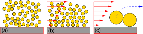
Figure 1: A schematic two-dimensional illustration showing the effect of shear flow on the microstructure of hard spheres at a hard wall. (a) A typical equilibrium configuration. (b) Shear flow leads to the formation of layers in the $xz$-plane as particles at different values of $y$ attempt to overtake each other. (c) Focusing on a binary collision close to the wall. The particle closer to the wall gets pushed against it, while the colliding particle is forced to ‘roll around’ the other in order to move past.

III Interaction-flow coupling

In the present work we wish to study the influence of flow on a fully interacting, inhomogeneous system. So far, the only application of (6) has been to spherically inhomogeneous systems subject to a variety of flow fields rauscher1 ; mk_diploma ; dzubiella ; rauscher2 ; rauscher3 (representing a single colloid in a sea of ideal or Gaussian polymers). In particular, under shear flow, the ideal particles accumulate at the colloid surface within the two compressive quadrants ($I\equiv{\bf r}\cdot(\boldsymbol{\kappa}+\boldsymbol{\kappa}^{T})\cdot{\bf r}<0$) and are depleted from the extensional quadrants ($I>0$), leading to ‘wake’ formation at larger shear rates mk_diploma . The advected DDFT (6) thus captures a certain coupling between inhomogeneities in the density field and external flow. However, this ‘external potential-flow coupling’ is a straightforward consequence of employing an external potential (e.g. a fixed sphere) which either directly obstructs the particles as they attempt to follow the affine flow, or perturbs the solvent flow field such that the particles are swept around the obstacle (when the appropriate Stokes flow is employed).

A more demanding and illuminating test of the advected-DDFT approach is provided by considering external potentials which do not directly hinder the affine path of the advected particles, but which may nevertheless be expected to generate flow dependent density profiles. Emphasis may thus be placed upon the nontrivial ‘interaction-flow coupling’. For the purpose of the present work we will thus focus on the special case of a time-independent external potential which varies in $y$-direction and restricts the particles to move in the half space

$$V^{\rm ext}({\bf r})=\begin{cases}\;\infty\hskip 56.9055pty<d/2\\ \;V^{\rm ext}_{w}(y)\hskip 34.42802pty>d/2.\end{cases}$$ (10)

The translational invariance of $V^{\rm ext}_{w}$ within the $xz$-plane has the consequence that the resulting equilibrium density distribution varies in $y$-direction only. In addition to the external potential field, we specialize the external flow field to a steady simple shear with flow in $x$-direction and a linear gradient in the $y$-direction

$$\mathbf{v}=y\,\dot{\gamma}\,\hat{\mathbf{e}}_{x},$$ (11)

with shear rate $\dot{\gamma}$ (corresponding to a velocity gradient tensor $\kappa_{\alpha\beta}=\dot{\gamma}\delta_{\alpha x}\delta_{\beta y}$). The pair potential entering (9) represents a hard-sphere repulsion

$$\phi(r)=\begin{cases}\;\infty\hskip 42.67912ptr<d\\ \;\;0\hskip 45.52458ptr>d.\end{cases}$$ (12)

The situation under consideration is shown schematically in the second panel of Fig.1. Note that the zero-shear plane may be located at $y=0$ without loss of generality, as only relative particle velocities are physically relevant.

Application of (6) to treat the specified nonequilibrium situation immediately reveals the problem at hand. We have already noted that our chosen geometry leads to translational invariance of the equilibrium density distribution within the $xz$-plane, $\rho_{\rm eq}({\bf r},t)=\rho_{\rm eq}(y,t)$. For the shear flow (11) the advective term in (6) is thus given by

$$\nabla\cdot(\rho({\bf r},t)\mathbf{v}({\bf r},t))=\nabla\cdot(y\,\dot{\gamma}\,\rho(y,t)\,\hat{\mathbf{e}}_{x})=0.$$ (13)

Within the advected-DDFT approach the applied shear flow has no influence on the density profile at the wall. Equation (6) thus reduces to (4), which, for the present time-independent external potential, yields the equilibrium density profile. This disappointing conclusion contradicts physical intuition and presents a fundamental failing of Eq.(6).

In the right panel of Fig.1 we sketch what we consider to be the correct physical picture. As a shear flow is applied parallel to the wall the particles experience a (nonconservative) force proportional to their perpendicular separation from the wall. Particles at different values of $y$ thus seek to move past each other, perturbing the equilibrium microstructure and leading, at higher shear rates, to the formation of particle layers in the $xz$-plane. In particular, when a pair of particles collide close to the wall, the particle at smaller $y$ will be forced against the wall, whereas the second particle will be forced to roll around its neighbour in order to follow as closely as possible the affine solvent flow. These physical mechanisms should be manifest in the nonequilibrium density profile.

We note that Brownian dynamics simulations brady_rev display two dimensional particle layering at intermediate shear rates, followed by an additional symmetry breaking in the vorticity direction at high shear rates, characterized by the formation of particle chains in $x$-direction. It is important to realize that the density distribution described by DFT represents an average over all $z$-coordinates of the particle chains (which, for an infinite system, are not pinned to a particular location in $z$). Our assumption that $\rho({\bf r},t)=\rho(y,t)$ is thus fully justified for the present density functional based study.

IV Mean field theory

In a system without HI, $N$-particle configurations for which colloidal particles overlap are forbidden by the infinitely repulsive colloidal pair potential. While an exact statistical mechanical treatment (i.e. exact evaluation of the integral in (5)) would lend such unphysical configurations zero statistical weight, care must be exercised in approximate treatments which do not fully satisfy this important geometrical constraint. In the present situation it would appear that application of the equilibrium sum rule (5) does not satisfy exactly the no-overlap ‘core condition’ when applied to driven states. However, it is not at all clear how to improve the approximation (5) in a way that both incorporates the flow induced distortion of $\rho^{(2)}({\bf r}_{1},{\bf r}_{2},t)$ and enables its weighted integral to be approximated using an equilibrium free energy functional. For this reason we take an alternative route and attempt to include the missing physics by modifying the advective term in (6). This approach is motivated by considering the dynamics of hydrodynamically interacting dispersions.

In a system with HI, the hydrodynamic velocity entering (8) can be decomposed into affine and particle induced fluctuation terms ${\bf v}_{i}(t)=\boldsymbol{\kappa}(t)\cdot{\bf r}_{i}+{\bf v}^{\rm fl}_{i}(t)$, where ${\bf v}^{\rm fl}_{i}(t)$ can be expressed in terms of the third rank hydrodynamic resistance tensor lubrication . The fluctuation term describes the disturbance of the affine solvent flow by the particles and ensures that a pair of approaching particles ‘flow around’ each other, without coming into direct contact. The impenetrable character of the particles, represented by the pair potential (12), thus enters indirectly by providing a boundary condition for the solvent flow. Integration of (7) over $N\!-\!1$ degrees of freedom yields an advective term

$$\nabla\cdot\,\rho({\bf r},t)[\,\boldsymbol{\kappa}(t)\cdot{\bf r}\,+\,{\bf v}^{\rm fl}({\bf r},t)\,]$$ (14)

where ${\bf v}^{\rm fl}({\bf r},t)\equiv\langle{\bf v}^{\rm fl}_{i}(t)\rangle$ is the conditional average over $N\!-\!1$ coordinates, given that a particle is located at ${\bf r}$. In contrast to (13), the divergence in (14) is not neccessarily zero for the inhomgeneous system presently under consideration. For hydrodynamically interacting systems the fluctuation term may thus provide the desired contribution to the flux in $y$-direction.

The above considerations suggest a possible solution to the problem posed by (13). By empirically incorporating a conditionally averaged fluctuation term into the velocity field driving our Brownian system, we aim to mimic the hydrodynamic fluctuation term discussed above. In this way we can correct, at least to some extent, the occurance of unphysical overlaps by enforcing that there be no radial flux between pairs of particles at contact. We envisage a system of hard-core particles under shear flow in which there occur frequent and random binary collisions. At each collision the particles rotate around each other according to some specified rule (for our specific choice, see section V below) before moving apart along their respective streamlines. For a homogeneous system, this mechanism gives rise to zero net flux through any given plane at constant $y$. However, in the presence of the external potential field (10), the inhomogeneous density distribution will lead to a $y$-dependent flux which will modify the equilibrium distribution, until it is balanced by an equal and opposite diffusive flux, thus establishing a nonequilibrium steady state.

As the density profile under consideration varies only in $y$-direction, we need only seek the $y$-component of the fluctuation contribution. The arguments presented above thus suggest the mean field term

$$v^{\rm fl}_{y}(y,t)=\int_{-\infty}^{\,\infty}dy^{\prime}\rho(y^{\prime},t)\,\bar{v}^{k}_{y}(y-y^{\prime})$$ (15)

which expresses the contribution of the density at $y^{\prime}$ to the average velocity at $y$. The ‘flow kernel’ $\bar{v}^{k}_{y}(y)$ entering (15) describes the $y$-component of the velocity of a particle which collides with a neighbour at vertical separation $y$. Our modified version of (6) thus becomes

$$\frac{\partial\rho(y,t)}{\partial t} = \frac{\partial}{\partial y}\Bigg{[}\,-\rho(y,t)v^{\rm fl}_{y}(y,t)$$ (16)

$$\hskip 14.22636pt+\;\;\;Pe^{-1}\rho(y,t)\frac{\partial}{\partial y}\frac{\delta\mathcal{F}[\rho(y,t)]}{\delta\rho(y,t)}\Bigg{]},$$

where we have scaled length using $d$ and time using $\dot{\gamma}$, leading to an explicit appearance of the Peclet number, $Pe\equiv\dot{\gamma}d^{2}/D_{0}$, expressing the competition between affine advection and diffusive motion. The steady state solution of (16) is given by

$$\rho(y)=z\exp\left(-\beta V^{\rm ext}(y)+c^{(1)}(y)+Pe\!\int_{y}^{\infty}\!\!\!dy^{\prime}v^{\rm fl}_{y}(y^{\prime})\right)$$

(17)

where $z$ is the equilibrium fugacity and we have introduced the one-body direct correlation function bob_advances

$$c^{(1)}({\bf r})=-\frac{\delta\beta\mathcal{F}[\rho({\bf r},t)]}{\delta\rho({\bf r},t)}.$$ (18)

The integral in (17) can be regarded as a nonequilibrium contribution to the intrinsic chemical potential. It should be noted that the requirement that a homogeneous density generates no particle flux in $y$-direction implies that the spatial integral over $v_{y}(y)$ is zero. For homogeneous states $v_{y}^{\rm fl}(y,t)$ is thus zero and the bulk chemical potential is unchanged from that in equilibrium.

V Flow kernel

In order to derive the flow kernel in Eq. (15), we consider the relative velocities of two particles, a tagged particle with position $\mathbf{r}_{t}$ and a reference particle at $\mathbf{r}_{r}$, during a scattering event, with $\Delta\mathbf{r}=\mathbf{r}_{t}-\mathbf{r}_{r}$. As discussed above, we neglect hydrodynamic interactions to keep the description as simple as possible. The incorporation of hydrodynamic interactions should in principle be possible in our approach. The following derivation of the scattering velocities is based on the assumption that in any situation, the particles adjust their velocities such that they minimize the friction with the solvent. The particles are at contact while they move around each other and then pass each other (see the right panel of Fig.1). During the contact period, they have a nonvanishing velocity relative to the solvent. We will now derive the velocity $\mathbf{v}^{k}$ of the tagged particle in the frame comoving with the reference particle, which is assumed to move with constant velocity $\dot{\gamma}y_{r}$, i.e., we keep $y_{r}$ fixed. In a real scattering event one particle would move up and the other down. In our mean field picture, where the tagged particle moves in the fixed density distribution of other particles, we have to keep the $y$-position of the reference particle fixed. The velocity with minimal friction follows from minimization of the velocity relative to the solvent velocity $\mathbf{v}$, which we denote $\Delta{\bf v}$,

$$\Delta v^{2}=(\mathbf{v}^{k}-\mathbf{v})^{2}=(v^{k}_{x}-\dot{\gamma}\Delta y)^{2}+v_{y}^{k2}+v_{z}^{k2}.$$ (19)

As long as the particles are in contact, they move on a trajectory with constant distance from each other, leading to

$$\Delta r^{2}=d^{2}.$$ (20)

Differentiation of this expression and elimination of $\Delta x$ leads to

$$v^{k}_{x}=-\frac{v^{k}_{y}\Delta y+v^{k}_{z}\Delta z}{\sqrt{d^{2}-\Delta y^{2}-\Delta z^{2}}}.$$ (21)

Inserting in Eq. (19) yields

$$\Delta v^{2}=\left(-\frac{v^{k}_{y}\Delta y+v^{k}_{z}\Delta z}{\sqrt{d^{2}-\Delta y^{2}-\Delta z^{2}}}-\dot{\gamma}\Delta y\right)^{2}+v_{y}^{k2}+v_{z}^{k2}.$$ (22)

We can now minimize this expression with respect to $v^{k}_{y}$ and $v^{k}_{z}$. This yields,

$$v^{k}_{y}(\Delta y,\Delta z)=-\dot{\gamma}\left(\frac{\Delta y}{d}\right)^{2}\sqrt{d^{2}-\Delta y^{2}-\Delta z^{2}}.$$ (23)

In order to average this value over all possible values of $\Delta z$, we substitute

$$\Delta z=\sqrt{d^{2}-\Delta y^{2}}\sin\phi.$$ (24)

into (23) and integrate over $\phi$ to obtain (the factor of $\frac{1}{2\pi}$ is inserted as normalization, and the range of the integral is restricted to the half circle since the velocity is zero for $|\phi|>\pi/2$)

$$v^{k}_{y}(\Delta y) =-\frac{1}{2\pi}\dot{\gamma}\left(\frac{\Delta y}{d}\right)^{2}\sqrt{(d^{2}-\Delta y^{2})}\int_{-\pi/2}^{\pi/2}\!\!\!\!d\phi\cos\phi$$

$$=-\frac{\dot{\gamma}}{\pi}\left(\frac{\Delta y}{d}\right)^{2}\sqrt{d^{2}-\Delta y^{2}}.$$ (25)

This result does not account for the density of particles at contact, relative to that in bulk. In order to include information about the local microstructure about a reference particle, the flow distorted inhomogeneous pair distribution function $g({\bf r},y)$ should, in principle, be included as a prefactor in (23) before angular integration. Given that $g({\bf r},y)$ is not known, we make the zeroth order approximation $g({\bf r},y)=g_{\rm eq}(r)$, to arrive at our final result

$$\bar{v}^{k}_{y}(\Delta y)=-\frac{\dot{\gamma}}{\pi}\,g_{\rm eq}(d)\left(\frac{\Delta y}{d}\right)^{2}\sqrt{d^{2}-\Delta y^{2}}.$$ (26)

For hard-spheres the Carnahan-Starling expression $g_{\rm eq}(d)=(1-\phi/2)/(1-\phi)^{3}$ provides a simple and accurate expression for the contact value hansen . For other choices of interaction potential $g_{\rm eq}(d)$ may be obtained using either integral equation methods brader_ijtp or, more consistently, an equilibrium test-particle calculation employing the same Helmholtz free energy as that used to generate the dynamics.

VI Excess free energy

Given the equation of motion (16) and flow kernel (26), we need to specify a particular approximation to the excess free energy functional in order to arrive at a closed theory for the density profile. For hard-sphere fluids the Rosenfeld functional rosenfeld yields accurate results for both the microstructure and thermodynamics. Within the Rosenfeld approximation the excess free energy of hard-spheres is given by

$$\mathcal{F}^{\rm hs}_{\rm ex}[\rho] = -n_{0}\ln(1-n_{3})\,+\,\frac{n_{1}n_{2}-\boldsymbol{n}_{1}\cdot\boldsymbol{n}_{2}}{1-n_{3}}$$ (27)

$$+\,\frac{n_{2}^{3}-3n_{2}(\boldsymbol{n}_{2}\cdot\boldsymbol{n}_{2})}{24\pi(1-n_{3})^{2}}.$$

where the weighted densities are given by convolutions of the density profile

$$n_{\alpha}(\mathbf{r})=\int d\mathbf{r^{\prime}}\rho(\mathbf{r^{\prime}})\,\omega^{(\alpha)}(\mathbf{r}-\mathbf{r^{\prime}}).$$ (28)

The weight functions are characteristic of the geometry of the particles

$$\omega^{(3)}(\mathbf{r}) = \Theta(r-R),$$

$$\omega^{(2)}(\mathbf{r}) = \delta(r-R),$$

$$\omega^{(1)}(\mathbf{r}) = \frac{\delta(r-R)}{4\pi R},$$

$$\omega^{(0)}(\mathbf{r}) = \frac{\delta(r-R)}{4\pi R^{2}},$$

$$\boldsymbol{\omega}^{(2)}(\mathbf{r}) = \frac{\mathbf{r}}{r}\delta(r-R),$$

$$\boldsymbol{\omega}^{(1)}(\mathbf{r}) = \frac{\mathbf{r}}{r}\frac{\delta(r-R)}{4\pi R},$$ (29)

where $R=d/2$ is the sphere radius. Although improved versions of the Rosenfeld functional do exist roth_review , the original version rosenfeld will prove sufficient for the present application.

VII Results

VII.1 Hard-spheres

We first address the problem of hard-spheres at a hard wall ($V^{\rm ext}_{w}(y)=0$). The steady state equation (17) was solved numerically (Picard iteration) using the flow kernel (26) and the Rosenfeld approximation to the excess free energy. The contact value of the radial distribution function employed in (26) was taken from the Carnahan-Starling equation of state hansen .

VII.1.1 Intermediate shear rates

In Fig.2 we show density profiles calculated for a volume fraction $\phi=0.45$ at various (low to intermediate) values of the Peclet number. In equilibrium, $Pe=0$, the density profile shows a typical oscillatory structure arising from local packing contraints at the wall. Applying a finite $Pe$ leads to an increase in both the contact value (see inset (a)) and height of the oscillatory peaks, which is accompanied by an increase in the depth of the minima. The enhanced structure of the profile is a direct consequence of the collision mechanism built into the advective term of our theory (c.f. Fig.1.c) and indicates the development of particle layers in nonequilibrium steady states at finite $Pe$. Despite the highly structured character of the nonequilibrium profiles, it should be noted that the adsorption (i.e. the spatial integral of $\rho(y)-\rho_{b}$) remains independent of $Pe$, where $\rho_{b}=\frac{6\phi}{\pi d^{3}}$ is the bulk colloid density. While this is a straightforward consequence of the continuity equation underlying (6), it nevertheless provides a useful check for our numerical results.

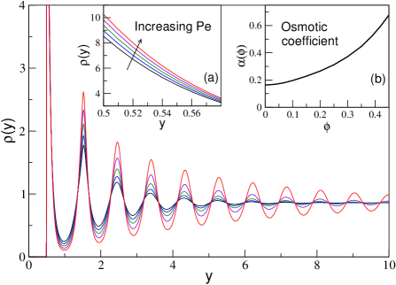
Figure 2: Steady state density profiles of a hard-sphere fluid at volume fraction $\phi=0.45$ for $Pe=0,3.142,6.283,9.425$ and $12.566$. As the Peclet number is increased the oscillatory structure of the profile becomes more pronounced, reflecting the formation of particle layers in the $xz$-plane. Inset (a) focuses on the region close to the wall, where the contact value $\rho(d/2)$ increases linearly with $Pe$. Inset (b) shows the density dependence of the coefficient determining the nonequilibrium contribution to the reduced osmotic pressure $\beta\Pi_{\rm ne}(\phi,Pe)=\alpha(\phi)\phi^{2}Pe$, as determined from the contact value.

VII.1.2 Osmotic pressure

For hard-spheres at a hard-wall, the contact value of the density profile satisfies the sum rule

$$\beta\Pi=\rho(d/2),$$ (30)

where $\Pi$ is the osmotic pressure. While the sum rule (30) is generally applied to equilibrium, there seems to be no reason why it should not be equally valid for the present nonequilibrium situation (although, as far as we are aware, there currently exists no mathematical proof of this assertion). Our numerical calculations show that, for a given volume fraction, the contact value $\rho(d/2)$ increases linearly over a the entire range of Peclet numbers investigated ($Pe=0\rightarrow 10$ for each volume fraction considered). Employing the sum rule (30) we thus find that the numerically obtained osmotic pressure obeys the following relation

$$\beta\Pi(\phi,Pe)=\beta\Pi_{\rm eq}(\phi)+\alpha(\phi)\phi^{2}Pe$$ (31)

where $\alpha(\phi)$ is a volume fraction dependent coefficient.

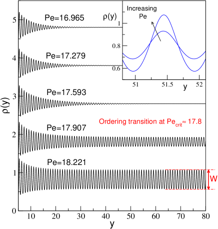
Figure 3: Steady state density profiles for volume fraction $\phi=0.42$ at $Pe=16.965,17.279,17.593,17.907$ and $18.221$. For clarity the profiles have been translated vertically. As $Pe$ is increased the profiles display an increasingly slow oscillatory decay to the bulk density. At a critical value of $Pe=Pe_{\rm crit}$ the Brownian motion is no longer able to restore the equilibrium structure far from the wall and shear effects dominate. For $Pe>Pe_{\rm crit}$ the oscillations no longer decay and the entire sample enters a layered state, characterized by a well defined oscillation amplitude. The width of the laning oscillations away from the wall (and which extend throughout the entire sample) defines an order parameter $W$ characterizing the nonequilibrium transition. The inset focuses on a single peak ($\phi=0.42$) within the layering region for $Pe=17.907$ and $18.221$. The layering peaks can be well approximated by a Gaussian.

The definition of $\alpha(\phi)$ in the second term of (31) is motivated by the exact low volume fraction results of Brady and Morris brady_morris . By solving exactly the pair Smoluchowski equation in the low density limit for hard-spheres without HI it has been shown that the osmotic pressure (obtained from the trace of the stress tensor) is given by

$$\beta\Pi(\phi\rightarrow 0,Pe)=\rho_{b}+\frac{4}{3\pi^{2}}\phi^{2}Pe$$ (32)

In inset (b) of Fig.2 we show the volume fraction dependence of $\alpha$. Gratifyingly, the fact that $\alpha$ exhibits a low volume fraction plateau confirms that the present theory indeed captures the correct scaling ($\sim\phi^{2}Pe$) of the flow induced correction to the osmotic pressure. The fact that we recover the correct low density scaling is a nontrivial output of our approach. However, the limiting value $\alpha(\phi\rightarrow 0)=0.164$ obtained in the present work differs from the exact value of $4/3\pi^{2}=0.135$ by a factor of $1.2$. Given the rather severe approximations employed in the present work, namely the mean-field term (15) and flow kernel (26), it should not be surprising that there is some deviation from the exact result. Nevertheless, the recovery of the correct low density scaling is reassuring and suggests that performing calculations with a renormalized Peclet number $Pe^{*}=Pe/1.2$ may be appropriate, should a detailed comparison with simulation or experiment be required.

We note that time-dependent solutions of (16) (not considered in the present work) would enable study of the transient behaviour of the Osmotic pressure resulting from time-dependent changes in the applied shear flow, e.g. the onset of steady shear flow zausch .

VII.1.3 Laning transition

Turning now to higher values of $Pe$, we show in Fig.3 density profiles for $\phi=0.42$ and $Pe=16.695\rightarrow 18.221$, focusing on the layering structure away from the direct vicinity of the wall (the region $y>5$ is shown). As $Pe$ is increased from zero to values around $17.6$ the oscillatory structure shows an increasingly slow decay with distance from the wall, indicating that Brownian motion is gradually succumbing to the influence of the applied shear flow. For $Pe>17.6$ the decay length of the oscillatory profiles shows a strong sensitivity to variations in the Peclet number and diverges at a critical value $Pe_{\rm crit}\approx 17.8$. This divergence signifies the onset of an ordered phase for which the asymptotic density profile is characterized by a well defined period and amplitude of oscillation.

The emergence of an infinitely extended oscillatory profile at a critical value of the Peclet number is a nontrivial prediction of the present theory and signifies a non equilibrium transition to an inhomogeneous steady state. Such layered states have been observed in Brownian dynamics simulations foss_brady but have thus far remained inaccessable to microscopically based theories. For $Pe>Pe_{\rm crit}$ it is of interest to look at the structure of the individual oscillations within the layered phase. In the inset to Fig.3 we show a single density peak at $y\approx 51.4$ for $Pe=17.907$ and $18.221$. For larger values of $Pe$ the peak becomes both narrower and higher, reflecting the reduced influence of Brownian motion, which acts to damp the oscillations and restore equilibrium. The density peaks in the layering region may be well approximated by a Gaussian, implying the existence of two-dimensional particle planes at high $Pe$ values, with harmonic restoring forces acting against random out-of-plane fluctuations.

Shear induced layering phases, similar to those predicted by the present theory, have been observed in both colloidal experiments hoffman1 ; hoffman2 ; ackerson_clark ; ackerson_pusey ; ackerson and Brownian dynamics simulations of hard-sphere dispersions foss_brady . More recently, experiments on noncolloidal dispersions (no Brownian motion) under oscillatory shear have shown that the presence of irreversible processes when the particles collide can give rise to self-organization and the formation of particle lanes pine .

VII.1.4 Phase diagram

The oscillation amplitude of the density in the limit $y\rightarrow\infty$ serves as an order parameter characterizing the nonequilibrium transition from a locally layered state, homogeneous in bulk, to a fully macroscopic layered phase. Specifically, $W\equiv\max(\rho(y\rightarrow\infty))-\min(\rho(y\rightarrow\infty))$ provides a suitable order parameter (see Fig.3). In Fig.4 we show the nonequilibrium phase diagram in the $(\phi\,,Pe)$ plane, obtained by examination of $W$ as a function of $Pe$. For each volume fraction density profiles were calculated on a large grid extending beyond $300$ particle diameters. For $Pe<Pe_{\rm crit}$ the converged profiles clearly decay to zero as a function of $y$, well within our sample size (as for the profiles for $Pe=16.965,17.279$ and $17.593$ in Fig.3). For $Pe>Pe_{\rm crit}$ iteration of Eq.(17) results in a ‘laning region’ which grows out from the wall indefinitely until the laning structure covers the entire range of the numerical grid. The value of $W$ for laning states may thus be operationally defined as the density difference between the minina and maxima of the oscillations at a distance sufficiently far removed from the wall. In practice, $W$ was estimated from the variation of the profile around $y=150$. The inset to Fig.4 shows $W$ as a function of $Pe$ for $\phi=0.42$, following the path indicated by an arrow in the main figure. For values of $Pe$ close to, but above, the transition, $W$ is well described by a square root.

The phase diagram shown in Fig.4 is consistent with that calculated in Brownian dynamics simulations of charge stabilized colloidal dispersions (see Fig.4 in grest ), provided that the temperature used in the simulation study is identified as an inverse volume fraction. In grest temperatures both above and below the equilibrium freezing transition were considered and the nonequilibrium order-disorder phase boundary found to vary continuously through the freezing transition. In the present study we prefer to restrict ourselves to volume fractions below freezing ($\phi_{\rm fr}=0.494$) in order to avoid the possible complications which may arise from the presence of underlying metastable states. A serious study of the complex interaction between crystal nucleation and external flow goes beyond the scope of the present work.

Finally, we note that the value $Pe_{\rm crit}=14.7$ obtained from the present theory for $\phi=0.45$ is remarkably consistent with Brownian dynamics simulations performed at the same volume fraction (c.f. Figure.3 in foss_brady ). The simulations predict that a layered structure emerges within the range $Pe=10\rightarrow 30$.

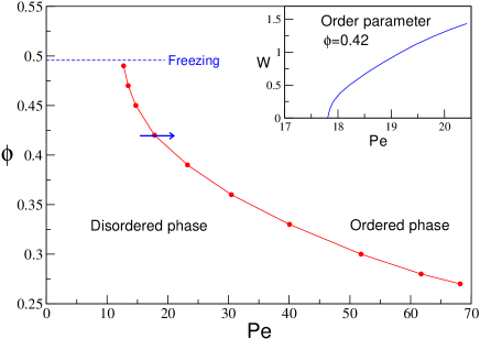
Figure 4: The phase boundary in the $(\phi\,,Pe)$ plane separating the disordered phase from the ordered ‘laning’ phase (lines serve as a guide for the eye between calculated data points). The hard-sphere freezing transition at $\phi=0.494$ is indicated by the broken line. The inset shows the order parameter $W$ as a function of $Pe$ for $\phi=0.42$, following the path indicated by the blue arrow in the main panel. Above $Pe_{\rm crit}$ the numerical data suggests a continuous transition with the order parameter varying as $W\sim(Pe\!-\!Pe_{\rm crit})^{\frac{1}{2}}$ for small $Pe\!-\!Pe_{\rm crit}$.

VII.1.5 Bulk laning

The results presented in the previous section indicate that the presence of the dynamical mean field term in (17) gives rise to an instability with respect to laning when the Peclet number exceeds a certain critical value. Although we have concentrated on the particular problem of particles at a hard-wall, it would appear that the density inhomogeneities induced by the wall simply serve to ‘seed’ the generation of a laning structure for $Pe>Pe_{\rm crit}$. It may thus be anticipated that for supercritical values of $Pe$, any kind of density fluctuation, regardless of its amplitude, will be sufficient to initiate laning.

In order to test the above hypothesis we have solved (17) for a range of $Pe$ numbers using the following initial guess for numerical iterative solution

$$\rho_{\rm init}(y)=\rho_{b}+a\exp(-b(y-y_{0})^{2}),$$ (33)

for various values of the parameters $a,b$ and $y_{0}$. For $Pe<Pe_{\rm crit}$ the perturbation is eroded during the iteration procedure and yields the steady state solution $\rho(y)=\rho_{b}$ for all values of the parameter set $(a,b,y_{0})$. For $Pe>Pe_{\rm crit}$ any finite value of the parameter $a$ is sufficient to seed the laning and a fully laned steady state solution, extending over the entire numerical sample length, is obtained, regardless of the values of $b$ and $y_{0}$ employed. In this sense, it would appear that, for supercritical states, any amount of ‘numerical dirt’ in the initial homogeneous density distribution is sufficient to generate a fully laned steady state. Moreover, we have confirmed that the values of $Pe_{\rm crit}$ thus obtained are entirely consistent with the phase boundary shown in Fig.4, which was calculated in the presence of a hard-wall. Given the above observations it would be of interest to perform a fully time-dependent solution of (16). Such a calculation, which we defer to a future publication, would also enable predictions to be made regarding the timescale upon which lanes are formed and its dependence upon the supersaturation $Pe\!-\!Pe_{\rm crit}$.

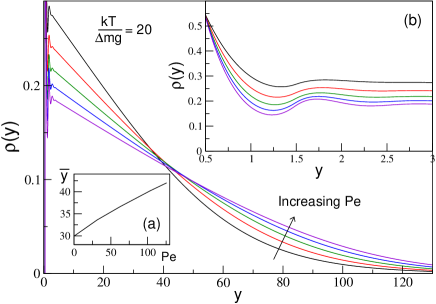
Figure 5: Steady state sedimentation profiles of a relatively dilute dispersion for $Pe=0,31.416,62.832,103.673$ and $125.664$ at a fixed value of the gravitational length $k_{B}T/g\Delta m=20$. The black curve corresponds to $Pe=0$ and is obtained from a static DFT calculation at a fugacity $z=1.5$. Due to the conservation equation underlying our DDFT, steady state profiles at finite $Pe$ have the same adsorption as the profile for $Pe=0$, i.e. particle number is conserved. Inset (a) shows the center-of-mass $\bar{y}$ (see Eq.36 as a function of $Pe$. Inset (b) focuses on the region close to the wall and demonstrates fact that the contact value is independent of $Pe$.

VII.2 Influence of gravity

We now consider adding an extra component to the external potential

$$V_{w}^{\rm ext}(y)=yg\Delta m,$$ (34)

where $\Delta m$ is the bouyant mass of a colloid and $g$ is the gravitational field strength. We thus address the influence of the shear flow (11) upon colloidal sedimentation profiles. Choosing a fugacity $z=1.5$ and gravitational length $\xi=k_{B}T/g\Delta m=20$ yields the equilibrium sedimentation profile shown in Fig.5, for which the local volume fraction remains rather low, even in the vicinity of the wall. As $y$ increases, the local packing oscillations give way to a monotonic decrease of the density. It may thus be anticipated that for finite values of $Pe$, the flow kernel built into our mean-field theory will lead to a net transport of particles from regions of high density to regions of lower density until the scattering flux is balanced by the gravity-biased diffusion of particles towards smaller $y$ values.

The expectation of flow induced broadening of the sedimentation profiles is confirmed by the steady state results shown in Fig.5. Note that the particle number (i.e. area under each of the curves in Fig.5) is conserved and is independent of $Pe$. The canonical nature of the DDFT imposes that the broadening of the sedimentation profile with increasing $Pe$ is accompanied by an overall decrease in the local density within the range $0<y<40$. It is interesting to consider this change of the density distribution in view of the recently discussed violation of the fluctuation dissipation theorem (FDT) Krueger09 ; Berthier02 in sheared systems. This violation was expressed in terms of the fluctuation dissipation ratio $X_{\rm FDT,f}$ defined as the ratio of response and thermal fluctuations for observable $f$ (see, e.g. Krueger09 for details). In equilibrium, one has $X_{\rm FDT,f}=1$, while under shear, $X_{\rm FDT,f}<1$ is observed. Since, by definition, the ratio $X_{\rm FDT,f}$ is proportional to $(k_{B}T)^{-1}$ (when keeping response and fluctuations $T$-independent), one can also describe the FDT violation in terms of an effective temperature $T_{\rm FDT,f}=T/X_{\rm FDT,f}$ which in turn is larger than $T$ Berthier02 . (Note that the dependence of $X_{\rm FDT,f}$, and hence $T_{\rm FDT,f}$, on observable $f$ is unclear.) Here, we are tempted to define in analogy the center-of-mass ratio $X_{\rm com}$,

$$X_{\rm com}=\frac{\bar{y}(0)}{\bar{y}(\dot{\gamma})},$$ (35)

with $\bar{y}(\dot{\gamma})$ the center-of-mass of the density distribution at shear rate $\dot{\gamma}$,

$$\bar{y}=\frac{\int_{0}^{\infty}\!dy\,y\rho(y)}{\int_{0}^{\infty}\!dy\,\rho(y)}.$$ (36)

At low density, $\rho(y)\propto\exp[-y/\xi]$ and $\bar{y}=\xi\propto k_{B}T$, independent of shear. At higher density, $\rho$ in Fig. 5 does not follow a simple exponential, but one still expects $\bar{y}(0)\propto k_{B}T$, as long as packing effects are not too dominant. This confirms the close analogy of our defintion of $X_{\rm com}$ to $X_{\rm FDT,f}$: if for the system under shear, the ratio $X_{\rm com}$ will be smaller than unity, one can formally interpret this in terms of an effective temperature larger than $T$. Inset (a) to Fig.5 shows that the center-of-mass under shear is indeed larger then in equilibrium, i.e., we indeed have $X_{\rm com}<1$ in accordance to the findings for the ratio $X_{\rm FDT,f}$. The decrease of $X_{\rm com}$ as function of shear rate resembles the behavior of $X_{\rm FDT,f}$, which was also found to decrease with shear rate Krueger09 ; Berthier02 . We furthermore expect that $X_{\rm com}$ decreases with density and note $X_{\rm com}\to 1$ for $\phi\to 0$ (where $\bar{y}(\dot{\gamma})\to\xi$), as observed for $X_{\rm FDT,f}$. The center-of-mass ratio hence shows the same overall properties as the fluctuation-dissipation-ratio. This suggests that both are driven by similar physical processes. These findings are also interesting in view of efforts towards a thermodynamic definition of an effective temperature of the system under shear Langer07 . We realize that a comparison of the concrete values of $X_{\rm com}$ and $X_{\rm FDT,f}$ is not possible since the system under gravity is different from the bulk-systems studied in Krueger09 ; Berthier02 ; Langer07 , as the density depends both on $y$ and $\dot{\gamma}$. Future work on a single tagged heavy particle in a bath of density matched particles might prove more useful in this respect.

Despite the broadening of the profiles as a function of $Pe$, the ultimate asymptotic decay can always be fitted by a Boltzmann decay, $\rho(y\rightarrow\infty)\sim\exp(-y/\xi)$. This is expected since the density far away from the wall is low and $\varrho(y)$ hence approaches the Boltzmann-distribution.

The inset to Fig.5 focuses on the region $0.5<y<3$. Despite the major changes in density distribution induced by the applied shear flow, it is striking that the contact value $\rho(d/2)$ remains independent of $Pe$, in contrast to our previous findings at $g=0$ (see Figs.2 and 3). This is not surprising. For any finite $g$, the steady state density profile has an adsorption $\Gamma\equiv\int_{0}^{\infty}\!dy\,\rho(y)$ corresponding to the average number of particles in a column in $y$-direction with unit area in the $xz$-plane. In a gravitational field this column of particles thus exerts a force $\Gamma g\Delta m$ on the wall and determines the contact value of the density distribution. As particle number is conserved within the DDFT, it follows that the contact value of the density at the wall will be independent of $Pe$, as observed in our numerical solutions. The fact that the variation in contact value as a function of $Pe$ is distictly different for the two cases $Pe=0$ and $Pe\neq 0$ is related to the singular behaviour of $\rho(y\rightarrow\infty)$ in the limit $g\rightarrow 0$.

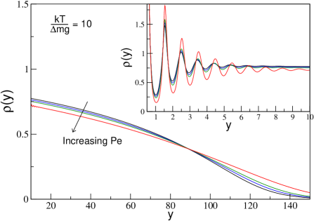
Figure 6: Steady state sedimentation profiles of a dense dispersion for $Pe=2,4,6$ and $15$ and at separations removed from the wall. The inset shows the local structure close to the wall. Although some local layering can be induced close to the wall at high shear rates, the gravitational force suppresses the development of an extended layering phase. As in Fig.5, the contact values remains independent of $Pe$.

Fig.6 shows further sedimentation profiles for a state with $\xi=10$ and larger local volume fraction than those shown in Fig.5. As previously, the profiles broaden with increasing $Pe$. Due to high local density in the vicinity of the wall, it may be expected that the layering transition identified in our calculations at $g=0$ may become relevant at sufficiently high $Pe$ values. The profile at the highest $Pe$ value shown in Fig.6 ($Pe=15$) does indeed show the development of a layering structure close to the wall, similar to that in Fig.2. However, the gravitational force acting on the particles supresses the development of long range oscillations and disrupts the formation of a macroscopic layering phase at any finite value of $Pe$. As for the profiles shown in Fig.5, the contact value at the wall remains independent of $Pe$ over the range of parameters investigated.

VIII Discussion

We have applied dynamical density functional theory to calculate the density profiles of a colloidal liquid at a wall under shear flow. The chosen flow geometry served to highlight failings of the existing DDFT approach to driven states and a semi-empirical correction was proposed to reintroduce the missing physical mechanism. Calculations performed at various volume fractions and Peclet numbers have revealed that the new approximation captures a non-equilibrium phase transition to an ordered laning state, for shear rates above a critical value of $Pe$. Moreover, sedimentation profiles are dramatically altered by the application of shear flow, which leads to an increase in height of the colloidal center-of-mass with increasing shear rate. The behavior of the center-of-mass ratio $X_{\rm com}$ is in qualitative agreement with the previously studied fluctuation-dissipation-ratio under shear. The study of a single tagged heavy particle in a bath of density matched particles might be an interesting variant for the future.

The mean-field correction to the advection term is presently rather empirical in character, arrived at using physical arguments, and it would be desirable to place this on a more rigorous basis, ideally as part of a systematic scheme for improving the DDFT under external flow. Whether this is possible remains to be seen. In some sense, the present state of the theory for driven states is reminiscent of the early days of equilibrium DFT, for which the first attempts to go beyond the local density or square gradient approximation relied on the introduction of empirical weight functions to incorporate spatial nonlocality bob_review . The insight gained from these studies proved very useful for the development of subsequent nonlocal approaches with a better foundation in statistical mechanics. We thus hope that the present work may provide stimulus for further developments in applying DDFT to driven nonequilibrium states.

The physical ’scattering’ mechanism built into the present theory generates a nontrivial coupling between density inhomogeneities and external flow, but has no effect on systems with a homogeneous density distribution. While this is likely to be appropriate for certain colloidal systems, it may represent an approximation for others. Imposing shear flow on a homogeneous dispersion generally leads to the development of finite normal stresses, which have been associated with the phenomenon of shear-induced particle migration morris_rev . It is thus conceivable that a shear-induced drift of particles to regions of lower shear rate could result in a density gradient through the sample. Very recent experiments on PMMA hard-sphere-like colloids suggest that flow-concentration coupling can lead to a novel form of shear-banding mike_banding . However, the banding reported in mike_banding only occurs for volume fractions above the glass transition, whereas the present work is focused purely on colloidal liquid states.

Both the standard form of DDFT (4) and its advected extension (6) are based on an implicit adiabatic assumption which neglects the time taken for the (one-time) pair correlation functions to equilibrate following a change in the average density profile. It may thus be anticipated that in very dense systems, for which the structural $\alpha$-relaxation time becomes important, the pair correlation functions will be unable to keep up with changes in the density, leading to a breakdown of the adiabatic approximation. The fact that the structural relaxation time of driven dense states is determined by the inverse flow rate $\dot{\gamma}^{-1}$ (at least for states with $\dot{\gamma}^{-1}<\tau_{\alpha}$) raises the interesting possibility that the adiabatic approximation may be more accurate when applied to calculate the response of dense systems to time-dependent changes in flow rate than to time-dependent changes in external potential. The present work has focused on steady state response and the next step in our research program will be to extend our studies to treat time-dependent shear flow.

An important simplification of the present treatment is that hydrodynamic interactions have been neglected. This excludes from the outset the development of the hydrodynamically bound clusters which may form at very high shear rates and which have been suggested as a possible mechanism for shear thickening joe_review . As we focus here on the low and intermediate Peclet numbers characteristic of the onset of shear thinning, this omission should not be too severe. More fundamental is the fact that the ordered phase observed in Brownian dynamics simulations foss_brady and captured by the present theory is apparently absent in Stokesian dynamics simulations including the full solvent hydrodynamics foss_brady2 . It would thus appear that hydrodynamic interactions can render the ordered phase unstable. Nevertheless, we consider it important that any prospective theory of driven colloids be able to descibe first the simpler case of interacting Brownian particles, before seeking to refine this to include hydrodynamics at some level. While it may well be that the (approximate) incorporation of hydrodynamic interactions into the theory disrupts the laning behaviour reported here, we can at least be sure that such an improved theory has a sound physical basis and that the laning observed in Brownian dynamics foss_brady will indeed emerge should we choose to switch-off the hydrodynamics. Such a gradual theoretical development, adding new physical aspects step-by-step, is important in developing a robust theory and tackling the fully hydrodynamic problem from the outset would be unlikely to deliver this.

References

- (1) R. Evans, Adv.Phys. 28 143 (1979);
- (2) R. Evans, in Fundamentals of inhomogeneous fluids, edited by D. Henderson (Dekker, New York, 1992).
- (3) Y. Rosenfeld, Phys.Rev.Lett. 63 980 (1989).
- (4) M. Schmidt, H. Löwen, J.M. Brader and R. Evans, Phys.Rev.Lett. 85 1934 (2000).
- (5) R. Evans, J. M. Brader, R. Roth, M. Dijkstra, M. Schmidt, and H. Löwen, Philos. Trans. R. Soc. London, Ser. A 359, 961 (2001).
- (6) J.M Brader, A. Esztermann and M. Schmidt, Phys.Rev.E 66 031401 (2002).
- (7) U. Marini Bettolo Marconi and P. Tarazona, J.Chem.Phys. 110 8032 (1999).
- (8) U. Marini Bettolo Marconi and P. Tarazona, J.Phys.: Condens.Matter 12 A413 (2000).
- (9) A.J. Archer and R. Evans, J.Chem.Phys. 121 4254 (2004).
- (10) Garnet Kin-Lic Chan and R. Finken, Phys.Rev.Lett. 94 183001 (2005).
- (11) P. Espanol and H.Löwen, J.Chem.Phys. 131 244101 (2009).
- (12) U. Marini Bettolo Marconi and S. Melchionna, J.Chem.Phys. 126 184109 (2007).
- (13) M. Rex and H. Löwen, Phys.Rev.Lett. 101 148302 (2008).
- (14) M. Rex and H. Löwen, Eur.Phys.J.E 28 139 (2009).
- (15) M. Rauscher, J.Phys.: Condens.Matter 22 364109 (2010).
- (16) M. Rex, H.H. Wensink and H. Löwen, Phys.Rev.E 76 021403 (2007).
- (17) H.H. Wensink and H. Löwen, Phys.Rev.E 78 031409 (2008).
- (18) M. Rauscher, A. Dominguez, M. Krüger and F. Penna, J.Chem.Phys. 127 244906 (2007).
- (19) J.M. Brader, M.E. Cates and M. Fuchs, Phys.Rev.Lett. 101 138301 (2008).
- (20) J.M. Brader, Th. Voigtmann, M. Fuchs, R.G. Larson and M.E. Cates, Proc. Natl. Acad. Sci. U.S.A. 106 15186 (2009).
- (21) M. Krüger and M. Rauscher, J.Chem.Phys. 127 034905 (2007).
- (22) M. Krüger, Diploma Thesis, University of Stuttgart, Germany 2006.
- (23) F. Penna, J. Dzubiella and P. Tarazona, Phys.Rev.E 68 061407 (2003)..
- (24) C. Gutsche, F. Kremer, M. Krüger, M. Rauscher, R. Weeber and J. Harting, J.Chem.Phys. 129 084902 (2007).
- (25) J. K. G. Dhont, An introduction to the dynamics of colloids (Amsterdam, Elsevier, 1996).
- (26) S. Kim and S.J. Karilla, Microhydrodynamics, principles and selected applications (Butterworth-Heinemann, Boston, 1991).
- (27) J.-P. Hansen and I.R. McDonald. Theory of Simple Liquids (Academic, London, 1986).
- (28) J.M. Brader, Int.J.Thermophys. 27 394 (2006).
- (29) R. Roth, J.Phys.:Condens.Matter 22 063102 (2010).
- (30) J.F. Brady and J.F. Morris, J. Fluid Mech. 348 103 (1997).
- (31) R.L. Hoffman, Trans.Soc.Rheol. 16 155 (1972).
- (32) R.L. Hoffman, J.Colloid Interface Sci. 46 491 (1974).
- (33) B.J. Ackerson and N.A. Clark, Phys.Rev.Lett. 46 123 (1982).
- (34) B.J. Ackerson and P.N. Pusey, Phys.Rev.Lett. 61 1033 (1988).
- (35) B.J. Ackerson, J.Rheol. 34 553 (1990).
- (36) D.R. Foss and J.F. Brady, J.Rheol. 44 629 (2000).
- (37) L. Corté, P.M. Chaikin, J.P. Gollub and D.J. Pine, Nature Physics, 4 420 (2008).
- (38) J. Zausch, J. Horbach, M. Laurati, S.U. Egelhaaf, J.M. Brader, T. Voigtmann and M. Fuchs, J.Phys.:Condens.Matter 20 404210 (2008).
- (39) J.F. Brady, Chem.Eng.Sci. 56 2921 (2001).
- (40) J.M. Brader, J.Phys.:Condens.Matter 22 363101 (2010).
- (41) W. Xue and G.S. Grest, Phys.Rev.Lett. 64 419 (1990).
- (42) J.F. Morris, Rheol.Acta 48 827 (2009).
- (43) R. Besseling, L. Isa, P. Ballesta, G. Petekidis, M.E. Cates and W.C.K. Poon, arXiv:1009.1579 (2010).
- (44) D.R. Foss and J.F. Brady, J.Fluid.Mech. 407 167 (2000).
- (45) M. Krüger and M. Fuchs, Phys. Rev. Lett. 102, 135701 (2009).
- (46) J. S. Langer and M. L. Manning, Phys. Rev. E 76, 056107 (2007).
- (47) L. Berthier and J.-L. Barrat, J. Chem. Phys. 116, 6228 (2002).