The statistical laws of popularity: Universal properties of the box office dynamics of motion pictures

Abstract

Are there general principles governing the process by which certain products or ideas become popular relative to other (often qualitatively similar) competitors ? To investigate this question in detail, we have focused on the popularity of movies as measured by their box-office income. We observe that the log-normal distribution describes well the tail (corresponding to the most successful movies) of the empirical distributions for the total income, the income on the opening week, as well as, the weekly income per theater. This observation suggests that popularity may be the outcome of a linear multiplicative stochastic process. In addition, the distributions of the total income and the opening income show a bimodal form, with the majority of movies either performing very well or very poorly in theaters. We also observe that the gross income per theater for a movie at any point during its lifetime is, on average, inversely proportional to the period that has elapsed after its release. We argue that (i) the log-normal nature of the tail, (ii) the bimodal form of the overall gross income distribution, and (iii) the decay of gross income per theater with time as a power law, constitute the fundamental set of stylized facts (i.e., empirical “laws”) that can be used to explain other observations about movie popularity. We show that, in conjunction with an assumption of a fixed lower cut-off for income per theater below which a movie is withdrawn from a cinema, these laws can be used to derive a Weibull distribution for the survival probability of movies which agrees with empirical data. The connection to extreme-value distributions suggests that popularity can be viewed as a process where a product becomes popular by avoiding “failure” (i.e., being pulled out from circulation) for many successive time periods. We suggest that these results may apply beyond the particular case of movies to popularity in general.

“Now that the human mind has grasped celestial and terrestrial physics, - mechanical and chemical, organic physics, both vegetable and animal, - there remains one science, to fill up the series of sciences of observation, - Social physics. This is what men have now most need of …” - Auguste Comte, The Positive Philosophy of Auguste Comte, tr. H Martineau, New York: Calvin Blanchard, 1855, p. 30.

I Introduction

As indicated by the above quotation from August Comte, the 19th century French philosopher and founder of the discipline of sociology, the idea of using the principles of physics to analyze and understand social phenomena is not new. Indeed, as Philip Ball has recently pointed out Ball03 , one can trace connections between physics and the study of socio-political phenomena back to the 16th century with the English philosopher, Thomas Hobbes. Hobbes, who had contributed, among other topics, to the physics of gases as well as to the theory of political science, believed that the deterministic principles of Galilean physics could be used to frame the laws governing not only the behavior of particles of matter but also that of particles of society, i.e., human beings. At about the same time an associate of Hobbes, William Petty, had appealed for an empirical study of society in the manner of physics, by measurement of quantifiable demographic and economic variables. This anticipated the use of statistical techniques to study society, which was eventually developed by the 19th century Belgian mathematician, Adolphe Quetelet. Quetelet’s book Essai de physique sociale (1835) outlined the concept of identifying the statistical characteristics of the “average man” by collecting data on a large number of measurable variables Quetelet42 . In fact, it is here the term “social physics” was used possibly for the first time to indicate the quantitative study of empirical data collected from a population. Its goal was to elucidate the statistical laws underlying social phenomena such as the incidence of crime or the rates of marriage. Quetelet used the Gaussian distribution, which had previously been introduced in the context of analysis of astronomical observations, to characterize many aspects of human behavior. Not surprisingly, this aroused great controversy among his contemporaries. There was an intense debate as to whether this meant that the freedom of choice for an individual was illusory. However, Quetelet was quite clear that this only implied an overall average tendency towards a certain behavior, rather than predicting how a specific individual will behave under a given set of circumstances. It is instructive that even today much of the opposition to the application of physics to study society is based on an erroneous impression that such an approach implies exact predictability of individual behavior.

Given the long historical connection between physics and the study of society, it is therefore surprising why more than a century has passed after the development of statistical physics before it was applied in a serious and sustained manner to analyze various social, economic and political phenomena. There have, of course, been several individual attempts in this direction earlier (e.g., see Ref. Mantegna05 ). The appealing parallels between the collective behavior of a large assembly of individuals, each of whose actions in isolation are almost impossible to predict, and that of a large volume of gas, where the dynamics of individual molecules are difficult to specify, have been noted even by non-physicists. For example, the science fiction writer, Isaac Asimov, has used this analogy as the basis for the fictional discipline of “psycho-history” in his Foundation series of novels where statistical laws describing the behavior of entire populations are used to predict the general historical outcome of events. It is of interest to note in this context that the framework of kinetic theory of gases has been used to explain certain universal socio-economic distributions, most notably, the distribution of affluence, measured in terms of either individual income or wealth Chatt07 ; Sinha09 .

However, it is only recently that there has been a large and concerted initiative by statistical physicists to explain social phenomena using the tools of their trade Castellano09 . This may be partly due to lack of sufficient quantities of high-quality data related to society. Indeed, the advances made in econophysics, i.e., the study of economic phenomena using the principles of physics, especially of properties pertaining to financial markets, have been attributed to the availability of large volumes of data. This has made it possible to quantitatively substantiate the existence of universal properties in the behavior of such systems, e.g., the inverse cubic law of the distribution of price fluctuations Gopikrishnan98 ; Lux96 ; Pan07 . These statistical laws, often referred to as “stylized facts” in the economic literature, are seen to be invariant with respect to different realizations of the system being studied.

More importantly, the existence of statistically universal behavior in socio-economic phenomena suggests that it may indeed be possible to explain them using the approach of physics, where the general properties at the systems-level need not depend sensitively on the microscopic details of its constituent elements. Indeed, it was the empirical observation that critical exponents of different physical systems are independent of the specific physical properties of their elementary components that gave rise to the modern theory of critical phenomena in statistical physics. The expectation that a similar path will be followed by the physics of socio-economic phenomena has driven the quest for empirical statistical laws governing such behavior, over the past decade and half Mantegna00 .

One of the areas of social studies where the search for statistical universal properties can be most fruitful is the emergence of collective decisions from the individual choice behavior of the agents comprising a group. Many such decisions have a binary nature, e.g., whether to cooperate or defect, to drop out of school, to have children out-of-wedlock, to use drugs, etc., which are reminiscent of the framework of spin models used to study cooperative phenomena in statistical physics Durlauf99 . The traditional economic approach to understand how such choices are made has been that every individual arrives at a decision based on the maximization of an utility function specific to him/herself and relatively independent of how other agents are behaving.

However, it has been clear for quite some time, e.g., through the work of Schelling on housing segregation Schelling78 , that in many, if not most such choice processes, an individual’s decision is influenced by those of its peers or members of its social network Wasserman94 ; Vega-Redondo07 . This interactions-based approach, where the social context is an important determinant of one’s choice, provides an alternative to utility maximization by individual rational agents in understanding several social phenomena. In particular, such an approach may be necessary for explaining the sudden emergence of a widely popular product or idea which is otherwise indistinguishable from its competitors in terms of any of its observable qualities. While traditional economic theory would hold that this suggests that there is a term in the utility function which corresponds to an unobservable property differentiating the popular entity from its competitors, there is no way of testing its scientific validity as such an hypothesis cannot be subjected to empirical verification. The alternative interactions-based viewpoint would be that, despite the absence of any intrinsic advantage initially, the chance accumulation of a relatively larger number of adherents early on would produce a slight relative bias in favor of adoption of a specific idea or product. Eventually, through a process of self-reinforcing or positive feedback via interactions, an inexorable momentum is created in favor of the entity that builds into an enormous advantage in comparison to its competitors (see, e.g., Ref. Arthur90 ).

While most such decisions do not have life-altering repercussions, the empirical study of collective choice dynamics can nevertheless result in formulation of statistical laws that may provide us with better understanding of, for instance, how financial manias sweep through apparently rational and highly intelligent traders or what leads to publicly sanctioned genocides in civilized societies. A relatively innocuous example of such choice behavior is seen in the emergence of movies that become extremely popular, often colloquially referred to as “superhits”, and its flip-side, the ignoble departure of intensely promoted movies which nevertheless fail miserably at the box-office. Frequently, it is not easy to see what quality differences (if any) are responsible for the runaway success of one and the mediocre performance of the others. It is thus a fecund area to search for signatures of statistical laws of popularity that can give us some indications of the essential dynamics underlying the emergence of collective decisions from individual choice.

In this paper, we have presented our results of a detailed analysis of the box-office performance of motion pictures released in theaters across the USA over the past several years, which are corroborated by data from India and Japan. The key finding reported here is that such choice dynamics has three prominent universal features which are invariant with respect to different periods of observations (and hence, different ensemble of movies). First, the gross income of a movie in its opening week, normalized by the number of theaters in which it is being shown, follows a log-normal distribution. Second, the number of theaters a movie is released in has a bimodal distribution. Together, these two properties account for the bimodal log-normal nature of the opening gross distribution for all movies released in a particular year. Further, we note that the total gross income of a movie over its entire theatrical run also follows a distribution that can be understood as a superposition of two log-normal distributions. The similarity between the opening and total gross distributions is related to the third universal feature of movie popularity, viz., the average gross weekly income per theater of a movie decreases as an inverse linear function of the time that has elapsed after its release. Together these three properties determine all observable characteristics of the movie ensemble, including the distribution of their lifetimes.

In section 2, we introduce the terminology used in the rest of the paper, discussing specific features of movie popularity and its quantifiable measures. This is followed by a short description of the data-sets that we have used for our analysis in section 3. In section 4, which describes our main results, first the properties of the distributions of the gross income, both for the opening week, as well as, over the total duration that a movie is shown in theaters, is discussed. We follow this up with results on the distribution of the number of theaters in which a movie is released, and try to see if any correlation exists between the opening and the overall performance of the motion picture at the box office. The time-evolution of a movie’s box-office performance is analyzed next. Our results show scaling in the decay of the income of a movie per theater as a function of time. In section 5, we discuss the distribution of persistence time (i.e., the duration up to which a movie is shown at theaters) which exhibits the properties of an extreme value distribution. This observation leads us to suggest that popularity can be viewed as a sequential survival process over many successive time periods, where a successful product or idea is one that survives being withdrawn from circulation for far longer than its competitors. We conclude with a conjecture that the invariant properties observed for movie popularity may also be relevant for other instances of popularity.

II Measuring movie popularity

For movies, as for most other products competing for attention by potential consumers/adopters, it is an empirically observed fact that only a very few end up dominating the market. As Watts points out “…for every Harry Potter and Blair Witch Project that explodes out of nowhere to capture the public’s attention, there are thousands of books, movies, authors and actors who live their entire inconspicuous lives beneath the featureless sea of noise that is modern popular culture” Watts03 . In fact, it is an oft-quoted fact about the motion picture industry that the majority of movies released every year do not attract enough viewers. The following comment made about Bollywood, the principal Indian film production and distribution system, applies also to motion picture industries worldwide: “fewer than 8 out of the more than 800 films made each year [in Bollywood] will make serious money” Torgovnik03 .

It may be worth mentioning here that popularity can arise through different processes. For example, a product can become a runaway success immediately upon release, its popular appeal presumably being driven by a saturation advertising campaign across different media that precedes the release. This has been the dominant marketing strategy for successful big budget movies which are collectively referred to as “blockbusters”. In contrast, products that are unsuccessful, referred to as “bombs” or “flops” in the context of movies, get a relatively poor reception on being released in the market. For such movies, a bad opening week is usually followed by ever-declining ticket sales resulting in a quick demise at the box-office. However, an alternative scenario is also possible where, after a modest opening week performance, a movie actually shows an increase in its popularity over subsequent periods. This process is thought to be driven by word-of-mouth promotion of the product through the social network of consumers who influence the choice of their friends and acquaintances. As more people adopt or consume the product, its popular appeal is increased further in a self-reinforcing process. These kinds of popular products, often termed “sleeper hits” in the context of movies, are much less frequent relative to the blockbusters and the bombs.

As in any quantitative study of the emergence of collective decision concerning the adoption of a product or an idea, the first question we need to resolve is how to measure popularity. While in some cases it may be rather obvious, as for example, the number of people driving a particular brand of car or practising a particular religion, in other cases it may be difficult to identify a unique measurable property that will capture all aspects of popularity. In particular, the popularity of movies can be measured in a number of ways. For example, we can look at the average ratings given by critics in reviews published in various media, web-based voting in different movie-related online forums, the cumulative number of DVDs rented (or bought) or the income from the initial theatrical run of a movie in its domestic market.

Let us consider in particular the case of movie popularity as judged by votes given by registered users of one of the largest online movie-related forums, the Internet Movie Database (IMDb) imdb . Voters can rate a movie with a number between 1-10, with 1 corresponding to “awful” and “10” to excellent. The cumulative distribution of the total votes for a movie approximately fits a log-normal distribution towards the tail, with the maximum likelihood estimates of the distribution parameters being $\mu=8.60$ and $\sigma=1.09$ Pan06 . However, the use of such scores as an accurate measure of movie popularity has obvious limitations. For instance, the different scores may be just a result of voters having differing amounts of information about the movies, with older, so-called classic movies clearly distinguished from newly released movies in terms of the voters’ knowledge about them. More importantly, as it does not cost anything to vote for a particular movie in such online forums, the vital element of competition for viewers that governs which product/idea will eventually become popular is missing from this measure. Therefore, we will focus on the box-office gross earnings of movies after they are newly released in theaters as a measure of their relative popularity. As we are considering only movies in their initial theatrical runs, the potential viewers have roughly similar kind of information available about the competing items. Moreover, such “voting with one’s wallet” is possibly a more honest indicator of individual preference for movies. The availability of large, publicly accessible data-sets of the daily or weekly earnings of movies in different countries in several movie-related websites has now made this kind of analysis a practical exercise.

III Data Description

For our study we have concentrated on data from the three most prolific feature film producing nations in the world: India, USA and Japan Hesmondhalgh07 . For example, of the 4,603 feature films produced around the world in 2005, India produced 1,041, USA 699 and Japan 356screendigest06 . While the US film industry, centered at Hollywood, has led the rest of the world for many decades both in terms of financial investment and the revenues generated by the films they make, India has been for a long time the largest producer of movies with a correspondingly high cinema admission. In fact, India accounts for almost a quarter of the total number of feature films made annually worldwide. Both India and USA have large domestic markets for their films, with locally produced movies having more than $90\%$ of the market share in each country. In addition, the US film industry also dominates the international market, with most cinemas around the world showing movies made in Hollywood.

For detailed information on the gross box office receipts for movies released across theaters in USA during the period 1999-2008, we have used the data available from the websites of The Movie Times movietimes and The Numbers numbers . The opening and total gross incomes of 5,222 movies released over this period have been considered in our analysis, as well as the maximum number of theaters in which they were shown. This roughly corresponds to including the 500-600 top earning movies for each year. We have used this data to obtain the overall distributions of movie popularity measured in terms of income. To compare the performance of a movie with its production budget, the latter information was obtained for 1,420 movies released over the period 2000-2008. We have also looked at the time-evolution of popularity, focusing on the approximately top 300 movies each year for the period 2000-2004. This corresponds to a total of 1497 movies over the five-year period, where the total gross receipt at the box office for each movie being considered is greater than $10^{5}$ USD. For these movies, we collected information about the gross income on each week during the time the film ran in theaters, as well as, the number of theaters that a movie was shown on a particular week.

For verifying the universal nature of the distributions obtained from the US data, we also considered the gross income data of a total of 500 movies released across theaters in India during the period 1999-2008 (corresponding to the top 50 movies each year in terms of their box-office income) that was obtained from the IbosNetwork web-site ibos . We also collected income data for 1095 movies released in Japan over the period 2002-2008 from the web-site BoxOfficeMojo boxofficemojo , which roughly corresponds to the 150 top earning films each year.

IV Results

IV.1 Distribution of Opening and Total Gross

As mentioned earlier, we will consider the gross income of a movie after it is released at theaters as a measure of its popularity, as this is directly related to the number of people who have been to a cinema to watch it. Thus, the total gross of a movie ($G_{T}$), i.e., the entire revenue earned from screenings over the entire period that it was shown in theaters, is a reasonable indicator of the overall viewership. An important property to note about the distribution of popularity for movies, measured in terms of their income, is that it deviates significantly from a Gaussian form in having a much more extended tail. In other words, there are many more highly popular movies than we would expect from a Normal distribution. This immediately suggests that the process of emergence of popularity may not be explained simply as an outcome of many agents independently making binary (viz., yes or no) decisions to adopt a particular choice, such as, going to see a particular movie. As this process can be mapped to a random walk, we expect it to result in a Gaussian distribution which, however, is not observed empirically. To go beyond this simple conclusion and identify the possible processes involved behind the emergence of popularity, one needs to ascertain accurately the true nature of the distribution of gross income.

The total gross is, of course, an aggregate measure of the box-office performance of a movie. Over the theatrical lifetime of a movie, i.e., the period between the time a movie is released to the time that it is withdrawn from the last theater it is being shown at, its viewership can show remarkable up- and down-swings. For example, two movies which have the same total gross can take very different routes to this overall performance. One movie may have opened at a large number of theaters and generated a large gross in its opening week followed by rapidly declining box-office receipts before being withdrawn. The other movie could have been initially released at a smaller number of theaters but, as a result of increasing popularity among viewers, was then subsequently released at more theaters and ran for a longer period, eventually garnering the same total gross. Thus, considering the opening gross of a movie ($G_{O}$), i.e., the box-office revenue on the opening week, can provide us with information about its popularity which complements that we have from its total gross. Indeed, the opening week is considered to be the most critical event in the commercial life of a movie as is evident from the pre-release publicity efforts of major Hollywood studios to promote movies in an effort to guarantee large initial viewership. This is because the opening gross is widely thought to signal the success of a particular movie. The observation that about 65-70$\%$ of all movies earn their maximum box-office revenue in the first week of release Vany99 appears to support this line of thinking. In the following analysis, we will look at both the total and the opening gross.

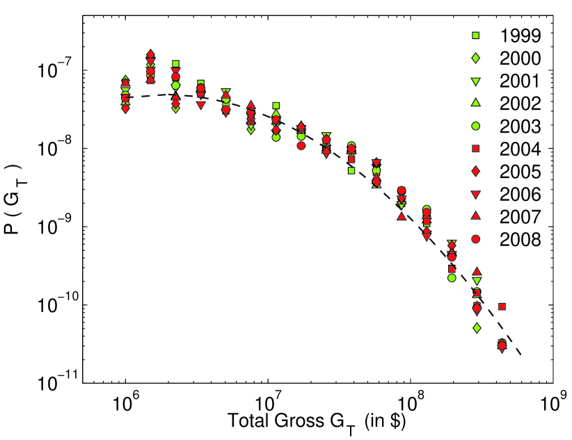
Figure 1: Probability distribution of the total gross income, $G_{T}$, for movies released across theaters in USA for each year during the period 1999-2008. The best fit for the aggregated data by a log-normal distribution (broken curve) with maximum likelihood estimated parameters $\mu=16.607\pm 0.062$ and $\sigma=1.471\pm 0.042$, is shown for comparison. The estimates of the log-normal distribution parameters for each individual year lie within error bars of the aggregate distribution parameters.

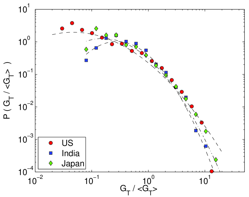
Figure 2: Probability distribution of the total gross income, $G_{T}$, scaled by the average total gross $\langle G_{T}\rangle$ of all movies released across theaters in (a) USA during the period 1999-2008, (b) India during the period 1999-2008 and (c) Japan during the period 2002-2008, each fit by a log-normal distribution (broken curves). The maximum likelihood estimates of the parameters for the log-normal fits to the scaled total gross are (a) $\mu=-0.901\pm 0.062$ and $\sigma=1.471\pm 0.042$ for USA, (b) $\mu=-0.436\pm 0.084$ and $\sigma=0.922\pm 0.056$ for India and (c) $\mu=-0.644\pm 0.076$ and $\sigma=1.097\pm 0.051$ for Japan. For the unscaled data (i.e., $G_{T}$), the corresponding MLE parameters are (i) $\mu=18.264\pm 0.084$ and $\sigma=0.922\pm 0.056$ for India, and (ii) $\mu=15.725\pm 0.076$ and $\sigma=1.097\pm 0.051$ for Japan.

Previous studies of movie income distribution Vany99 ; Sornette99 ; Vany03 had looked at limited data sets and found some evidence for a power-law fit. A more rigorous analysis using data for a much larger number of movies released across theaters in the USA was done in Ref. Sinha04 . While the tail of the distribution for the opening, as well as, the total gross for movies, may appear to follow an approximate power law $P(I)\sim I^{-\alpha}$ with an exponent $\alpha\simeq 3$ Sinha04 ; Sinha05 , an even better fit is achieved with a log-normal form (as shown in Fig. 1):

$$P(x)=\frac{1}{x\sigma\sqrt{2\pi}}e^{-({\rm ln}x-\mu)^{2}/2{\sigma}^{2}},$$ (1)

where $\mu$ and $\sigma$ are parameters of the distribution, being the mean and standard deviation of the variable’s natural logarithm. The maximum likelihood estimates of the log-normal distribution parameters for the aggregated US gross income data are $\mu=16.607$ and $\sigma=1.471$. The log-normal form has also been verified by us for the income distribution of movies released in India and Japan (Fig. 2). It is of interest to note that a strikingly similar feature has been observed for the popularity of scientific papers, as measured by the number of their citations, where initially a power law was reported for the probability distribution with exponent $\simeq 3$ but was later found to be better described by a log-normal form Redner98 ; Redner04 .

Table 1: Comparison between Kolmogorov-Smirnov statistics for the fitting of the tails of total gross ($G_{T}$) distribution with (a) log-normal and (b) power-law forms. The parameters for the best-fit log-normal distribution ($\mu$ and $\sigma$) and power-law distribution ($\alpha$) are obtained from maximum likelihood estimation. The value of $G_{T}^{min}$ (in currency units: INR for India and USD for USA & Japan) indicates the minimum total gross beyond which log-normal or power-law fitting is applied to the tail of the empirical distribution. The value of $G_{T}^{min}$ is chosen such that the empirical and best-fit distributions are as similar as possible in terms of minimum KS statistics.

Country	Year(s)	Log-normal distribution				Power-law distribution
		$\mu$	$\sigma$	$G_{T}^{min}$	$p$-value	$\alpha$	$G_{T}^{min}$	$p$-value
	1999	16.446	1.427		0.786	3.953	$12.69\times 10^{7}$	0.956
	2000	16.574	1.484		0.452	2.554	$4.88\times 10^{7}$	0.001
	2001	16.615	1.486		0.517	2.553	$5.02\times 10^{7}$	0.192
	2002	16.569	1.468		0.779	3.465	$11.67\times 10^{7}$	0.784
USA	2003	16.708	1.480	$8\times 10^{6}$	0.248	3.519	$~{}9.56\times 10^{7}~{}$	0.336
	2004	16.659	1.511		0.542	2.751	$5.71\times 10^{7}$	0.666
	2005	16.702	1.434		0.333	2.628	$4.56\times 10^{7}$	0.489
	2006	16.577	1.469		0.115	2.848	$5.23\times 10^{7}$	0.285
	2007	16.567	1.477		0.670	2.093	$2.85\times 10^{7}$	0.012
	2008	16.657	1.488		0.242	3.833	$12.75\times 10^{7}$	0.800
India	1999-2008	18.264	0.922	$1\times 10^{7}$	0.395	2.296	$7.75\times 10^{7}$	0.001
Japan	2002-2008	15.725	1.097	$5\times 10^{6}$	0.074	2.232	$9.56\times 10^{6}$	0.000

To further establish that the log-normal curve indeed describes the tail of the income distribution better than a power-law, we have also tested for the significance of the fits using Kolmogorov-Smirnov (KS) statistics Clauset09 (Table 1). After calculating the KS statistic for the empirical distribution and the best-fit curve obtained by maximum likelihood estimation (for both log-normal and power-law distributions), we have generated ensemble of random samples having same size as the empirical data from the best-fit distributions and the KS-statistic is calculated for each such sample. The $p$-value is obtained by measuring the fraction of samples whose KS-statistic is greater than that obtained from the empirical data and a higher $p$-value indicates greater confidence in the fit with the theoretical distribution. We note from Table 1 that the tails of the distributions of total gross earned by movies released in USA for each year during 1999-2008 is well-described by a log-normal distribution as indicated by the relatively high $p$-values, as are the tails of the aggregated distributions for India and Japan (the tails correspond to movies earning in excess of 8 million USD for USA, 10 million INR for India and 5 million USD for Japan). By contrast, we have to reject the hypothesis that the Indian and Japanese distributions can be described by a power-law tail as the corresponding $p\leq 10^{-3}$. For USA, the annual distributions for most years between 1999-2008 appear to have high $p$-value when a power-law is fit to the tail (corresponding approximately to movies earning in excess of 50 million USD). However, a power-law fit to the tail of the aggregate distribution of the entire US data (comprising movies that earned more than 1.10 billion USD) with the maximum likelihood estimated exponent $\alpha\simeq 3.26$ gives a $p$-value of only about 0.024. Thus, as the power-law form agrees with data from only one of the three countries considered, and moreover, fits a smaller region of the tail of the empirical distributions compared to the log-normal curve, we consider the latter to be a more suitable choice for describing the income distribution of movies than the former.

Instead of focusing only at the tail (which corresponds to the top grossing movies), if we now look at the entire income distribution, we notice another important property: a bimodal nature. There are two clearly delineated peaks which corresponds to a large number of movies either having a very low income or a very high income, with relatively few movies that perform moderately at box-office (Fig. 3). The existence of this bimodality can often mask the nature of the distribution, especially when one is working with a small data-set. For example, De Vany and Walls, based on their analysis of the gross for only about 300 movies, had stated that log-normality could be rejected for their sample Vany96 . However, this assumed that the underlying distribution can be fit by a single unimodal form - an assumption that was quite clearly incorrect as evident from the histogram of their data. Our more detailed and comprehensive analysis with a much larger data-set shows that the distribution of the total gross is in fact a superposition of two different log-normal distributions:

$$P(x)=p{\cal P}(x,\mu_{1},\sigma_{1})+(1-p){\cal P}(x,\mu_{2},\sigma_{2}),$$ (2)

where ${\cal P}()$ represents the log-normal distribution while $p$ and $(1-p)$ are the relative weights of the two component distributions about the lower and higher income peaks, respectively. We observe in Fig. 3 that the best-fit for the total income data occurs when $p\simeq 0.7$.

Turning our focus now to the opening gross, we notice that its distribution also has a bimodal form which can be similarly represented as a superposition of two log-normal distributions with the relative weights of the two components being $p=0.55$ and $(1-p)=0.45$. The more equal contributions of the distributions about the lower and higher income peaks in the opening week, as compared to that for the total or aggregated income over the entire lifetime seen earlier, is possibly because many movies which open with high viewership rapidly decay in terms of popularity and exit from the cinemas within a few weeks. Thus, their short lifetime translates into poor performance in terms of the overall income and they do not contribute to the higher income peak for the bimodal total gross distribution. However, the total and opening gross distributions are qualitatively similar, suggesting that the nature of the popularity distribution of movies is decided at the opening week itself . In this context, it is interesting to note the recent finding that the long-term popularity of online content in web portals such as YouTube can be predicted to a certain extent by observing the access statistics of an item (e.g., a video) in the initial period after it has been posted by an user Szabo10 .

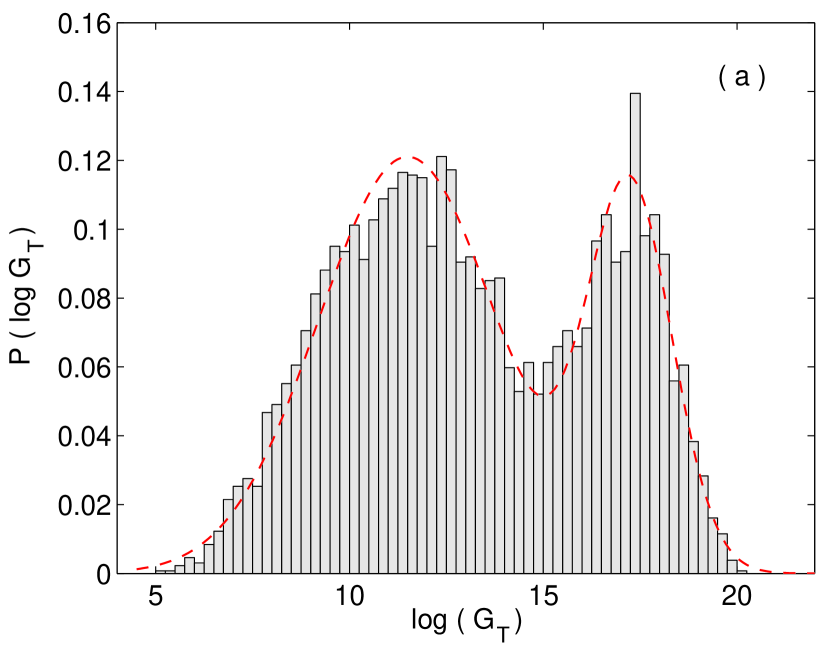
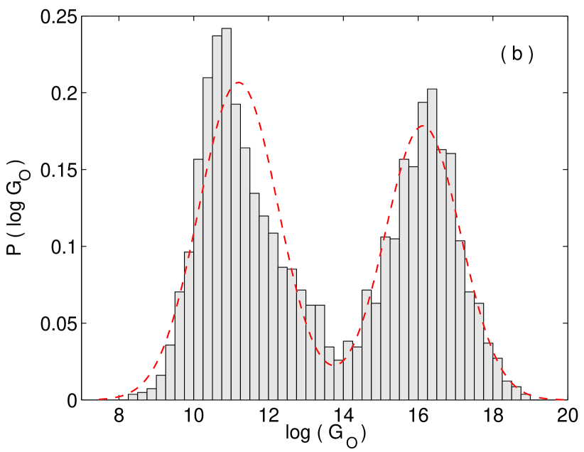
Figure 3: The logarithmically binned probability distributions for (a) the total gross, $G_{T}$, and (b) the opening gross, $G_{O}$, for movies released across theaters in USA during the period 1999-2008. Both distributions exhibit bimodal nature and have been fit using a superposition of two log-normal distributions ${\cal P}(x,\mu_{1},\sigma_{1})$ and ${\cal P}(x,\mu_{2},\sigma_{2})$ having relative weights $p$ and $(1-p)$, respectively. For the total gross, the best fit is obtained using $p=0.699$, $\mu_{1}=11.499$, $\mu_{2}=17.239$, $\sigma_{1}=2.305$ and $\sigma_{2}=1.089$, while for the opening opening gross, the best fit parameters are $p=0.549$, $\mu_{1}=11.199$, $\mu_{2}=16.126$, $\sigma_{1}=1.058$ and $\sigma_{2}=1.008$. Note that the data-set used for generating the distribution in (a) is larger than that used for (b), as there are some movies with low total gross whose opening week income is not available.

IV.2 Distribution of Gross per Theater

We now focus on understanding what is responsible for the bimodal log-normal distribution of the gross income for movies. It is, of course, possible that this is directly related to the intrinsic quality of a movie or some other attribute that is intimately connected to a specific movie (such as, how intensely a film is promoted in the media prior to its release). Lacking any other objective measure of the quality of a movie, we have used its production budget as an indirect indicator. This is because movies with higher budget would tend to have more well-known actors, better visual effects and, in general, higher production standards. As mentioned earlier, we have considered movies for which publicly available information about the production budget is available. This may not be the exact total cost incurred in making the movie, but nevertheless, gives an overall idea about the expenses involved. Fig. 4 (a) shows a scatter plot of the total gross as a function of the production budget for movies released between 1999-2008 whose budget exceeded 1 million dollars. As is clear from the figure, although in general, movies with higher production budget do tend to earn more, the correlation is not very high (the correlation coefficient $r$ is only 0.63). Thus, production budget by itself is not enough to guarantee high popularity. 

Another possibility is that the immediate success of a movie after its release is dependent on how well the movie-going public has been made aware of the film by pre-release advertising through various public media. Ideally, an objective measure for this could be the advertising budget of the movie. However, as this information is mostly unavailable, we have used as a surrogate the data about the number of theaters that a movie is initially released at. As opening a movie at each theater requires organizing publicity for it among the neighboring population, and, wider release also implies more intense mass-media campaigns, we expect the advertising cost to roughly scale with the number of opening theaters. As is obvious from Fig. 4 (b), the correlation between the opening gross per theater and the total number of theaters that a movie opens in is essentially non-existent (the correlation coefficient $r\simeq-0.15$), suggesting that advertising may not be a decisive factor for the the success of a movie at the box-office. In this context, one may note that De Vany & Walls have looked at the distribution of movie earnings and profit as a function of a variety of variables, such as, genre, ratings, presence of stars, etc. and have not found any of these to be significant determinants of movie performance Vany03 .

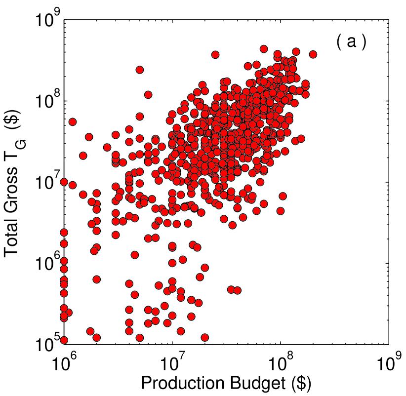
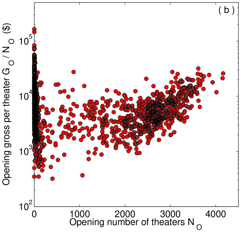
Figure 4: (a) Total gross ($G_{T}$) of a movie shown as a function of its production budget. The correlation coefficient is $r=0.633$ and the measure of significance $p<0.001$. (b) The opening gross per theater ($g_{O}=G_{O}/N_{O}$) as a function of the number of theaters in which a movie is released on the opening week. The correlation coefficient $r=-0.151$, with the corresponding measure of significance $p<0.001$.

Instead of focusing on factors inherent to specific movies that can be used to explain the gross distribution, we will now see whether the bimodal log-normal nature appears as a result of two independent factors, one responsible for the log-normal form of the component distributions and the other for the bimodal nature of the overall distribution. First, turning to the log-normal form, we observe that it may arise from the nature of the distribution of gross income of a movie normalized by the number of theaters in which it is being shown. The income per theater gives us a more detailed view of the popularity of a movie, compared to its gross aggregated over all theaters. It allows us to distinguish between the performance of two movies that draw similar number of viewers, even though one may be shown at a much smaller number of theaters than the other. This implies that the former is actually attracting relatively larger audiences compared to the other at each theater, and hence, is more popular locally. Thus, the less popular movie is generating the same income simply on account of it being shown in many more theaters, even though fewer people in each locality served by the cinemas may be going to see it.

Fig. 5 shows that the distribution of the gross income per theater over any given week, $g_{W}=G_{W}/N_{W}$, has a log-normal nature. Here, $G_{W}$ represents the total gross income of a movie over a week $W$ when it is being shown at $N_{W}$ theaters. Note that this is quite different from the earlier distributions because we are now considering together movies that are at very different stages in their lifetime. On a particular week, a few movies might have just opened, others are about to be withdrawn from exhibition, while still others are somewhere in the middle of their theatrical run. On the other hand, Fig. 6 shows the distribution of the income per theater of a movie on its opening week, i.e., $g_{O}=G_{O}/N_{O}$, where $N_{O}$ is the number of theaters in which the movie is released. Calculating the KS statistics for the log-normal fitting of the opening gross per theater gives a $p$-value of 0.678, indicating the fit to be statistically significant. Thus, both the distribution of $g_{W}$ and that of $g_{O}$ show a log-normal form despite the fact that they are quite different quantities, thereby underlining the robustness of the nature of the distribution.

The appearance of the log-normal distribution may not be surprising in itself, as it is expected to occur in any linear multiplicative stochastic process Mitzenmacher03 ; Ciuchi93 . The decision to see a movie (or not) can be considered to be the result of a sequence of independent choices, each of which have certain probabilities. Thus, the final probability that an individual will go to the theater to watch a movie is a product of each of these constituent probabilities, which implies that it will follow a log-normal distribution. It is worth noting here that the log-normal distribution also appears in other areas where popularity of different entities arise as a result of collective decisions, e.g., in the context of proportional elections Fortunato07 , citations of scientific papers Redner04 ; Radicchi08 and visibility of news stories posted by users on an online web-site Wu07 .

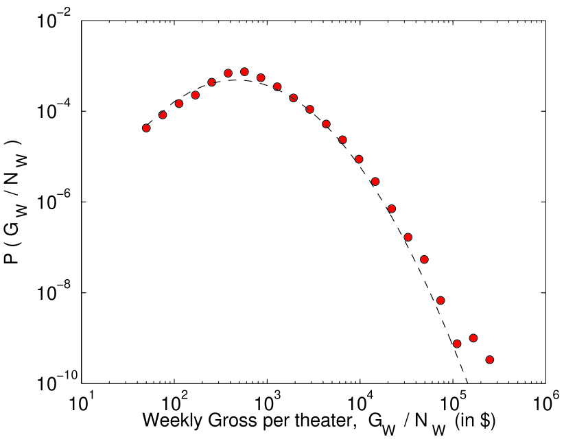
Figure 5: The probability distribution of $g_{W}(=G_{W}/N_{W})$, the gross income in a given week per theater for a movie released in USA during the period 2000-2004 fit by a log-normal distribution (broken curve). The parameters of the best-fit distribution are $\mu=7.208\pm 0.011$ and $\sigma=1.035\pm 0.008$. The data is averaged over all the weeks in the period mentioned.

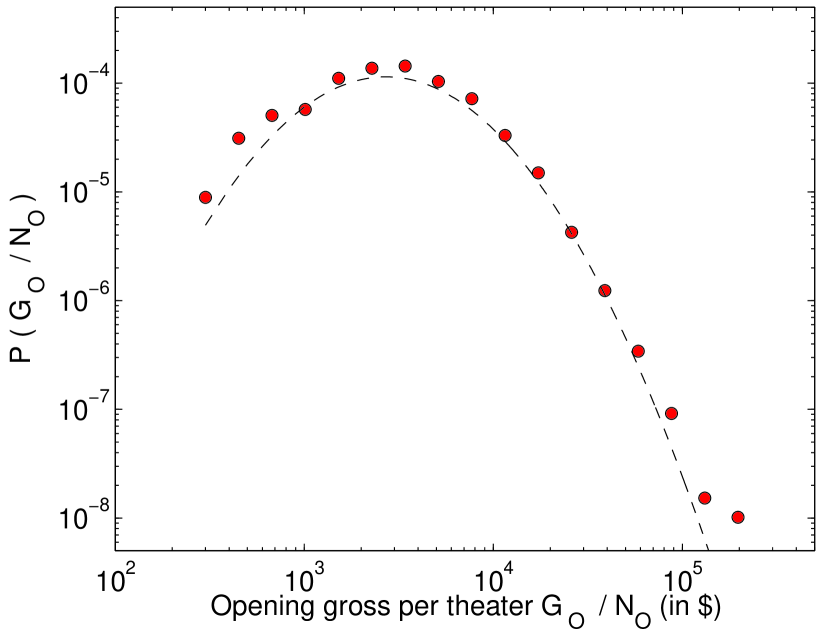
Figure 6: The probability distribution of $g_{O}(=G_{O}/N_{O})$, the opening week gross income per theater of a movie released in theaters across USA during the period 2000-2004 fit by a log-normal distribution (broken curve). The best-fit distribution parameters are $\mu=8.672\pm 0.044$ and $\sigma=0.877\pm 0.030$.

IV.3 Distribution of the number of theaters a movie is released

While the log-normal nature of the popularity distribution for movies (as measured by their gross income per theater) can be explained as the consequence of an underlying process where sequential stochastic choices are made by each individual to decide whether to watch the movie, its overall bimodal character is yet to be explained. Fig. 7 suggests a possible answer: the two peaks of the distribution of income may be reflecting the bimodality of the distribution of $N_{O}$, i.e., the number of theaters in which a motion picture is released, or of $N_{M}$, the largest number of cinemas that it plays simultaneously at any point during its entire lifetime. Thus, most movies are shown either at a handful of theaters, typically a hundred or less (these are usually the independent or foreign movies) or at a very large number of cinema halls, numbering a few thousand (as is the case with the products of major Hollywood studios). Unsurprisingly, this also decides the overall popularity of the movies to an extent, as the potential audience of a film running in less than a hundred theaters is always going to be much smaller than what we expect for blockbuster films. In most cases, the former will be much smaller than the critical size required to generate a positive word-of-mouth effect spreading through mutual acquaintances which will gradually cause more and more people to become interested in seeing the film. There are occasional instances where such a movie does manage to make the transition successfully, when a major distribution house, noticing an opportunity, steps in to market the film nationwide to a much larger audience and a “sleeper hit” is created. An example is the movie My Big Fat Greek Wedding, that opened in only 108 theaters in 2002 but went on to become the fifth highest grossing movie for that year, running for 47 weeks and at its peak was shown in more than 2000 theaters simultaneously.

Bimodality has also been observed in other popularity-related contexts, such as, in the electoral dynamics of US Congressional elections, where over time the margin between the victorious and defeated candidates have been growing larger Mayhew74 . For instance, the proportion of votes won by the Democratic Party candidate in the federal elections has changed from around 50$\%$ to one of two possibilities: either around 35-40$\%$ (in which case the candidate lost) or around 60-65$\%$ (when the candidate won). We have earlier proposed a theoretical framework for explaining how bimodality can arise in such collective decisions arising from individual binary choice behavior Pan06 ; Sinha06a ; Sinha06b . Individual agents took “yes” or “no” decisions on issues based on information about the decisions taken by their neighbors and were also influenced by their own previous decisions (adaptation), as well as, how accurately their neighborhood had reflected the majority choice of the overall society in the past (learning). Introducing these effects in the evolution of preferences for the agents led to the emergence of two-phase behavior marked by transition from a unimodal behavior to a bimodal distribution of the fraction of agents favoring a particular choice, as the parameter controlling the learning or global feedback is increased. In the context of the movie income data, we can identify this choice dynamics as a model for the decision process by which theater owners and movie distributors agree to release a particular movie in a specific theater. The procedure is likely to be significantly influenced by the previous experience of the theater and the distributor, as both learn from previous successes and failures of movies released/exhibited by them in the past, in accordance with the assumptions of the model. Once released in a theater, its success will be decided by the linear multiplicative stochastic process outlined earlier and will follow a log-normal distribution. Therefore, the total or opening gross distribution for movies may be considered to be a combination of the log-normal distribution of income per theater and the bimodal distribution of the number of theaters in which a movie is shown.

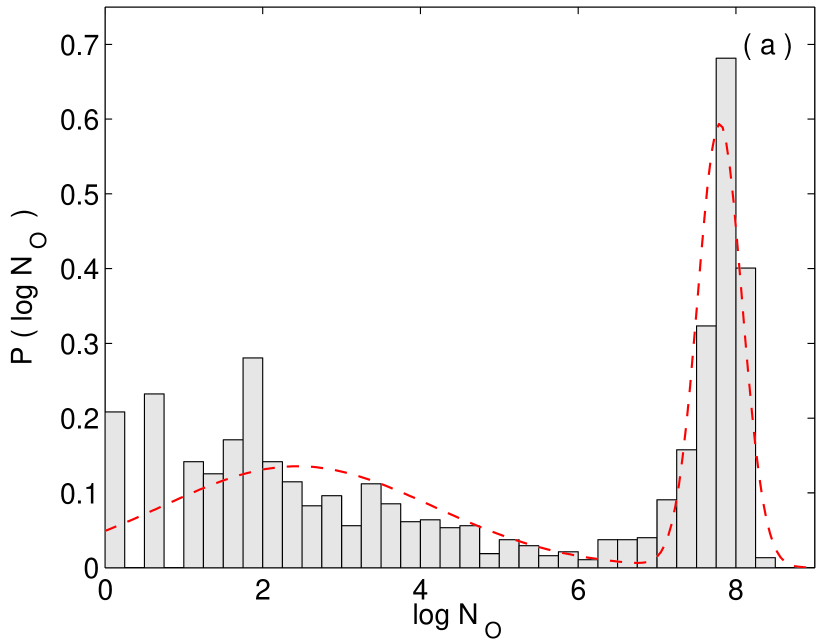
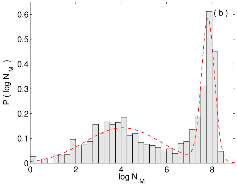
Figure 7: The probability distribution of the logarithm of (a) the number of theaters in which a movie is shown on its opening week, $N_{O}$, and (b) the largest number of theaters, $N_{M}$, that a movie is simultaneously shown on a given week in its entire lifetime. The data is for movies released across USA during 2000-2004. A fit using two Gaussian distributions is shown for comparison. The parameters of the best-fit distribution for the number of theaters in the opening week are $p=0.583$, $\mu_{1}=2.442$, $\mu_{2}=7.796$, $\sigma_{1}=1.714$ and $\sigma_{2}=0.281$, while that for the largest number of theaters in a week over its lifetime are $p=0.590$, $\mu_{1}=4.066$, $\mu_{2}=7.821$, $\sigma_{1}=1.651$ and $\sigma_{2}=0.285$.

IV.4 Time-evolution of movie popularity

The distribution of gross income analyzed so far represents a temporally aggregated view of the popularity of movies. As already mentioned, information about how the number of viewers change over time can reveal other aspects of the popularity dynamics, and in particular, can distinguish between movies in terms of how they have achieved their success at the box-office, viz., blockbusters and sleepers. This can be seen by looking at a plot of the total income of movies against their income in the opening week, with blockbusters having high values for both while sleepers would be characterized by a low opening but high total gross. One can also observe distinct classes of movies from the scatter-plot shown in Fig. 8 which indicates the correlation between the total gross income of a movie, representing its overall popularity, and its lifetime at the theaters, which is a measure for how long it manages to attract a sufficient number of viewers. We immediately notice that although many movies with high total gross also tend to have long lifetimes, there are also several movies which lie outside this general trend. Films which tend to have a very long run at the theaters despite not having as high a total income as major studio blockbusters may belong to a special class, e.g., effects movies which are made to be shown only at theaters having giant screens Sinha04 .

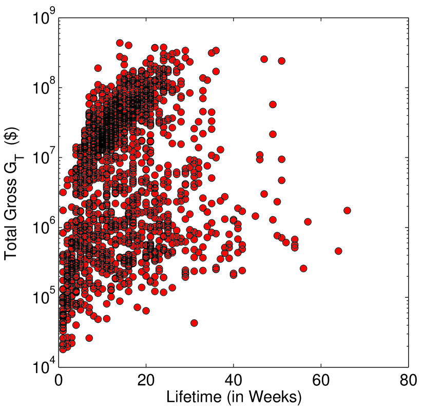
Figure 8: The total gross ($G_{T}$) earned by a movie as a function of its lifetime, i.e., the duration of its run at theaters. The correlation coefficient is $r=0.224$ with the corresponding measure of significance $p<0.001$.

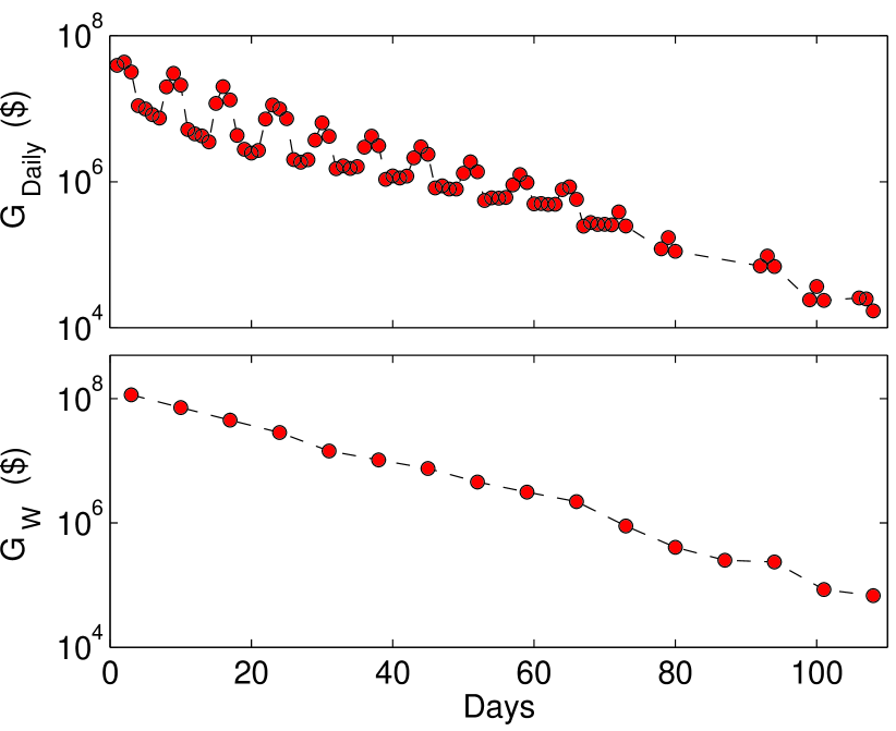
Figure 9: The time-evolution of (top) the daily gross income, $G_{Daily}$ (in dollars), and (bottom) the weekly gross income $G_{W}$ (in dollars) for the film Spiderman (released in 2002) aggregated over all theaters across USA. The gross income is seen to decay with time approximately exponentially, i.e., $\sim\exp(-\gamma t)$, where $\gamma\simeq 0.072$/day, giving a characteristic decay time of 14 days (i.e., 2 weeks).

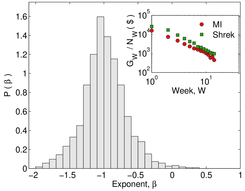
Figure 10: The distribution of exponents $\beta$ describing the power-law decay of the weekly gross income per theater, $g_{W}$ ($=G_{W}/N_{W}$) for all movies released in USA during 2000-2004 which ran in theaters for more than 5 weeks. The exponents were obtained by least-square linear fitting of the weekly gross income per theater of a movie as a function of time (measured in weeks, $W$) on a doubly-logarithmic scale. The inset shows the decay for two specific movies, Mission Impossible (1996) and Shrek (2001).

To go beyond the simple blockbuster-sleeper distinction and have a more detailed view of the time-evolution of movie popularity, one has to consider the trend followed by the daily or weekly income of a movie over time. Fig. 9 (top) shows that the daily gross income of a classic blockbuster movie, Spiderman (released in 2002) decays with time after release, having regularly spaced peaks corresponding to large audiences on weekends. To remove the intra-week fluctuations and observe the overall trend, we focus on the time series of weekly gross, $G_{W}$ (Fig. 9, bottom). This shows an exponential decay with a characteristic rate $\gamma$, a feature seen not only for almost all other blockbusters, but for bombs as well. The only difference between blockbusters and bombs is in their initial, or opening, gross. However, sleepers may behave differently, showing an initial increase in their weekly gross and reaching the peak in the gross income several weeks after release. For example, in the case of the movie My Big Fat Greek Wedding, the peak occurred 20 weeks after its initial opening. It is then followed by exponential decay of the weekly gross until the movie is withdrawn from circulation. Note that the exponential decay rate ($\gamma$) is different for different movies .

Instead of looking at the income aggregated over all theaters, if we consider the weekly gross income per theater, a surprising universality is observed. As previously mentioned, the income per theater gives us additional information about the movie’s popularity because a movie that is being shown in a large number of theaters may have a bigger income simply on account of higher accessibility for the potential audience. Unlike the overall gross that decays exponentially with time, the gross per theater of a movie shows a power-law decay in time measured in terms of the number of weeks from its release, $W$: $g_{W}\sim W^{-\beta}$, with exponent $\beta\simeq-1$ Sinha05 (see the inset of Fig. 10). This has a striking similarity with the time-evolution of popularity for scientific papers in terms of citations. It has been reported that the citation probability to a paper published $t$ years ago, decays approximately as $1/t$ Redner04 . Note that, Price Price76 had also noted a similar behavior for the decay of citations to papers listed in the Science Citation Index. In a very different context, namely, the decay over time in the popularity of a website (as measured by the rate of download of papers from the site) and that of individual web-pages in an online news and entertainment portal (as measured by the number of visits to the page), power laws have also been reported but with different exponent Sornette00 ; Dezso06 . More recently, relaxation dynamics of popularity with a power law decay have been observed for other products, such as, book sales from Amazon.com Sornette04 and the daily views of videos posted on YouTube Sornette08 , where the exponents appear to cluster around multiple distinct classes.

Fig. 10 shows the distribution of the power-law scaling exponents for all movies which ran for more than 5 weeks in theaters in USA during the period 2000-2004. Most of the movies have negative exponents, the mean and median being $-0.990$ and $-1.002$, respectively, indicating a monotonic decay in the income per theater as a reciprocal function of the time elapsed from the initial release date. Note that only 9 movies over the entire period analyzed by us had positive exponents and these had been shown at a very small number of theaters (around $5$ or less). For these movies the income per theater showed a slight increase towards the end of their lifetime before they were completely pulled out from theaters. On the whole, therefore, the local popularity of a movie at a certain point in time appears to be inversely proportional to the duration that has elapsed from its initial release.

V Discussion

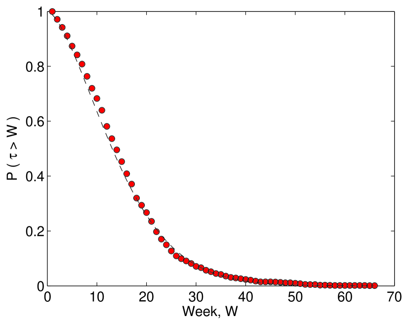
Figure 11: The cumulative persistence probability of a movie to remain in a theater for a period exceeding $W$ weeks shown as a function of time ($W$, in weeks) for movies released in USA during 2000-2004. The broken line shows a fit with the stretched exponential distribution (see text).

In the preceding section we have summarised the principal results from our analysis of the data on movie popularity as reflected in their gross income at the box office. One can now ask whether the three main features observed, viz., (i) log-normal distribution of gross per theater, (ii) bimodal distribution of the number of theaters a movie is shown at and (iii) the decay in gross per theater of a movie as an inverse function of the duration from its initial release, are sufficient to explain all other observable properties of movie popularity. To illustrate this we now consider an important quantifier not considered earlier: the persistence time of a movie, $\tau$, i.e., the duration upto which it is shown at theaters. As seen from Fig. 11, only about half of all the movies considered survive for beyond 14 weeks in theaters and only about $10\%$ persist beyond 25 weeks. The cumulative distribution fits a stretched exponential form ($\sim{\rm exp}[-(t/a)^{b}]$), indicating that the persistence time probability distribution can be described by the Weibull distribution Weibull51 :

$$P(t)=\frac{b}{a}\left(\frac{t}{a}\right)^{(b-1)}\exp\left[-\left(\frac{t}{a}\right)^{b}\right],$$ (3)

where $a,b>0$ are the shape and scale parameters of the distribution respectively. The best fit to the data shown in Fig. 11 is achieved for $a=16.485\pm 0.547$ and $b=1.581\pm 0.060$. The Weibull distribution is well-known in the study of failure processes and is often used to describe extreme events or large deviations. In particular, it has been applied to describe the failure rate of components, with the parameter $b>1$ indicating that the rate increases with time because of an aging process.

We can derive this empirical property of movie popularity from our earlier stated observations, with only an added assumption: that a movie is withdrawn from circulation when its gross income per theater falls below a critical value, $g_{c}$. An interpretation of this number is that it is related to the minimum number of tickets a theater has to sell per week in order to make the exhibition of the movie an economically viable proposition. Once the popularity of the movie has gone below this level, the theater is presumably no longer making a profit by showing this film and is better off showing a different movie. Therefore, the probability that the persistence time of a movie is $\tau$, is essentially given by the probability that the gross income per theater at time $\tau$ falls below $g_{c}$. To evaluate this probability, we use the observation that the gross per theater of a movie $i$ at any time $t$, $g^{i}_{t}$, has decayed by a factor $1/t$ (on average) from its initial value, $g^{i}_{O}$, i.e., the opening gross per theater. As the decay of gross income is not a completely deterministic process, we can express $g^{i}_{t}=(g^{i}_{O}/t)\eta$, where $\eta$ has a log-normal distribution with parameters $\mu$ ($=0$) and $\sigma$, which guarantees that the stochastic variation can never result in a negative value for the gross. If time is expressed in units of weeks ($j=1,2,\ldots$), the cumulative probability distribution of the persistence time $\tau_{i}$ is given by

$$P(\tau_{i}>T|g^{i}_{O})=\prod^{T}_{j=1}P(g^{i}_{j}>g_{c}|g^{i}_{O}),$$ (4)

which is a product of the probabilities that the gross income per theater earned by the movie in the $T$ successive weeks beginning from its initial release are all greater than the critical value $g_{c}$. We note that the right hand side expression of Eq. 4 is equal to $\prod^{T}_{j=1}P(\eta>g_{c}~{}j/g^{i}_{O}|g^{i}_{O})$, which is the product of cumulative distribution functions for the log-normal random variable $\eta$. Therefore, the cumulative distribution of the persistence time can be written as:

$$P(\tau_{i}>T)=\int_{0}^{\infty}P(g^{i}_{O})\prod^{T}_{j=1}\frac{1}{2}\left(1-{\rm erf}\left[\frac{{\rm ln}(g_{c}j/g^{i}_{O})}{\sqrt{2\sigma^{2}}}\right]\right)dg^{i}_{O},$$ (5)

where $P(g^{i}_{O})$ is the log-normal distribution of the opening gross per theater and ${\rm erf}(x)$ is the error function. Numerical solution of the above expression shows that it reproduces a stretched exponential curve, having reasonable agreement with the empirical data.

The fact that at least certain aspects of popularity dynamics can be described by the mathematical framework for understanding failure events is probably not a coincidence. A common observation across different areas in which popularity dynamics is operational is that most entities are pushed out of the market within a short time of their introduction. In many areas, this high rate of early extinction is balanced by new entrants into the market, so that at any given time, the number of competing entities is maintained more or less constant. Therefore, the key question in understanding popularity is why do most products or ideas fail to survive the brutal competition for being the most popular choice. We see instances of the general rule that “most things fail” in almost all types of economic phenomena Ormerod05 . As Ormerod has pointed out, of the 100 top business enterprises is 1912, 48 had ceased to exist as independent entities by 2005, while only 28 companies were larger (in real terms) than they were back in 1912. Similarly, out of the large number of computer software companies which had been in operation in the 1980s, only a handful have survived to the present. This is not just true for the present age but also for historical times. In 1469, twelve publishing houses had emerged in Venice in the (at that time) pioneering activity of printing books, but by the end of three years, only three of them had survived. Thus, a successful product is marked by its ability to survive in its early stages to build a consumer base. This may be a product of chance, as often there is little to distinguish between competitors in terms of their intrinsic qualities. However, once a product or idea has had a certain number of adherents, it is able to survive by the process of positive feedback, thereby generating more adherents. In the case of movies, the process reaches a natural limit when the potential audience is exhausted as everybody likely to view the movie has seen the film. In other cases, e.g., for religious or political ideas, the process can continue indefinitely as more and more converts are added to the fold. Thus, a general view of popularity dynamics can be expressed as follows: each competing product or idea, upon initial introduction to the market, has a certain probability of failing to attract a sufficient number of adherents. This means that at every successive time-step, the entity has to survive the possibility of early demise. A popular object, according to this view, is one which has repeatedly managed, by a combination of chance or design, to avoid failure (and subsequent exit from the marketplace) for far longer than its competitors.

VI Conclusions: The stylized facts of popularity

In this paper, we have analyzed the empirical data for movie popularity, measured in terms of its box-office income. We observe that the complex process of popularity can be understood, at least for movies, in terms of three robust features which (using the terminology of economics) we can term as stylized facts of popularity: (i) log-normal distribution of the gross income per theater, (ii) the bimodal distribution of the number of theaters in which a movie is shown and (iii) power-law decay with time of the gross income per theater. Some of these features have been seen in other instances in which popularity dynamics plays a role, such as, in citations of scientific papers or in political elections. This suggests that it may be possible that the above three properties may apply more generally to the processes by which a few entities emerge to become a popular product or idea. A unifying framework may be provided by the understanding of popular objects as those which have repeatedly survived a sequential failure process.

Acknowledgments

We would like to thank S Raghavendra, D Stauffer, J Kertesz, M Marsili and D Sornette for helpful comments at various stages. We gratefully acknowledge discussions with S V Vikram regarding the theoretical calculations in section 5. This work was supported in part by the IMSc Complex Systems (XI Plan) Project.

References

- (1) Ball P 2003 Complexus 1 190
- (2) Quetelet M A 1842 A Treatise on Man and the development of his faculties: An essay on Social Physics (Edinburgh: Chambers)
- (3) Mantegna R N 2005 Quant. Finance 5 133; Majorana E 2006 Scientific Papers Ed. Bassani G F (Bologna: Societa Italiana di Fisica) 250
- (4) Chatterjee A, Sinha S and Chakrabarti B K 2007 Current Science 92 1383
-
(5)
Sinha S and Chakrabarti B K 2009 Physics News (Bulletin of Indian Physics
Association) 39(2) 33, available from
http://www.imsc.res.in/~sitabhra/publication.html - (6) Castellano C, Fortunato S and Loreto V 2009 Rev. Mod. Phys. 81 591
- (7) Gopikrishnan P, Meyer M, Amaral L A N and Stanley H E 1998 Eur. Phys. J. B 3 139
- (8) Lux T 1996 Appl. Finan. Econ. 6 463
- (9) Pan R K and Sinha S 2007 Europhys. Lett. 77 58004
- (10) Mantegna R N and Stanley H E 2000 Introduction to Econophysics: Correlations and Complexity in Finance (Cambridge: Cambridge University Press)
- (11) Durlauf S N 1999 Proc. Natl. Acad. Sci. USA 96 10582
- (12) Schelling T C 1978 Micromotives and Macrobehavior (New York: Norton)
- (13) Wasserman S and Faust K 1994 Social Network Analysis: Methods and Applications (Cambridge: Cambridge University Press)
- (14) Vega-Redondo F 2007 Complex Social Networks (Cambridge: Cambridge University Press)
- (15) Arthur W B 1990 Scientific American 262(2) 92
- (16) Salganik M J, Dodds P S and Watts D J 2006 Science 311 854
- (17) Watts D J 2003 Six Degrees: The Science of a Connected Age (London: Vintage)
- (18) Torgovnik J 2003 Bollywood Dreams (London: Phaidon)
-
(19)
http://www.imdb.com - (20) Sinha S and Pan R K 2006 in Econophysics and Sociophysics: Trends and Perspectives (Weinheim: Wiley-VCH) 417
- (21) Hesmondhalgh D 2007 The Culture Industries (Sage)
-
(22)
World Film Production/Distribution 2006 Screen Digest (June) 205
http://www.screendigest.com -
(23)
http://www.the-movie-times.com -
(24)
http://www.the-numbers.com -
(25)
http://www.ibosnetwork.com -
(26)
http://www.boxofficemojo.com/intl/japan/ - (27) De Vany A and Walls W D 1999 J. Cult. Econ. 23 285
- (28) Sornette D and Zajdenweber D 1999 Eur. Phys. J. B 8 653
- (29) De Vany A 2003 Hollywood Economics (London: Routledge)
- (30) Sinha S and Raghavendra S 2004 Eur. Phys. J. B 42 293
- (31) Sinha S and Pan R K 2005 in Econophysics of Wealth Distributions (Milan: Springer) 43
- (32) Redner S 1998 Eur. Phys. J. B 4 131
- (33) Redner S 2004 Physics Today 58 49
- (34) Clauset A, Shalizi C R and Newman M E J 2009 SIAM Review 51 661
- (35) De Vany A and Walls W D 1996 Economic J. 106 1493
- (36) Szabo G and Huberman B A 2010 Comm. ACM 53 80
- (37) Mitzenmacher M 2003 Internet Math. 1 226
- (38) Ciuchi S, de Pasquale F and Spagnolo B 1993 Phys. Rev. E 47 3915
- (39) Fortunato S and Castellano C 2007 Phys. Rev. Lett. 99 138701
- (40) Radicchi F, Fortunato S and Castellano C 2008 Proc. Natl. Acad. Sci. USA 105 17268
- (41) Wu F and Huberman B A 2007 Proc. Natl. Acad. Sci. USA 104 17599
- (42) Mayhew D 1974 Polity 6 295
- (43) Sinha S and Raghavendra S 2006 in Practical Fruits of Econophysics (Tokyo: Springer) 200
- (44) Sinha S and Raghavendra S 2006 in Advances in Artificial Economics: The Economy as a Complex Dynamic System (Berlin: Springer) 177
- (45) Ratkiewicz J, Menczer F, Fortunato S, Flammini A and Vespignani A 2010 Phys. Rev. Lett. (to appear)
- (46) de Solla Price D J 1976 J. Am. Soc. Info. Sci. 27 292
- (47) Johansen A and Sornette D 2000 Physica A 276 338
- (48) Dezsö Z, Almaas E, Lukács A, Rácz B, Szakadát I and Barabási A-L 2006 Phys. Rev. E 73 066132
- (49) Sornette D, Deschatres F, Gilbert T and Ageon Y 2004 Phys. Rev. Lett. 93 28701
- (50) Crane R and Sornette D 2008 Proc. Natl. Acad. Sci. USA 105 15649
- (51) Weibull W 1951 J. Appl. Mech. 18 293
- (52) Ormerod P 2005 Why Most Things Fail: Evolution, Extinction and Economics (London: Faber & Faber)