Particle cosmology

Abstract

In these lectures the present status of the so-called standard cosmological model, based on the hot Big Bang theory and the inflationary paradigm is reviewed. Special emphasis is given to the origin of the cosmological perturbations we see today under the form of the cosmic microwave background anisotropies and the large scale structure and to the dark matter.

0.1 Introduction

There are fundamental questions we are on the edge of answering: what is the origin of our universe? Why is the universe so homogeneous and isotropic on large scales? What are the origins of dark matter and dark energy? What is the fate of our universe? While these lectures will certainly not be able to give definite answers to them, we shall try to provide the students with some tools they might find useful in order to solve these overwhelming mysteries themselves.

These lectures will contain a short review of the standard Big Bang model; a rather long discussion of the inflation paradigm with particular emphasis on the possibility that the cosmological seeds originated from a period of primordial acceleration; the physics of the Cosmic Microwave Background (CMB) anisotropies, and a short discussion of the dark matter

Since these lectures were delivered at a school, we shall not provide an exhaustive list of references to original material, but refer to several basic cosmology books and reviews where students can find the references to the original material [1, 2, 3, 4, 5, 6, 7, 8, 9, 10, 11].

0.2 Basics of the Big Bang model

The key starting point of the description of our universe is the fact that the latter looks homogeneous and isotropic on large scales. For such a reason the standard cosmology is based upon the maximally spatially symmetric Friedmann–Robertson–Walker (FRW) line element

$$ds^{2}=-dt^{2}+a(t)^{2}\left[{dr^{2}\over 1-kr^{2}}+r^{2}(d\theta^{2}+\sin^{2}\theta\,d\phi^{2})\right]\,;$$ (1)

Here $a(t)$ is the cosmic-scale factor; the curvature is parametrized by $R_{\rm curv}\equiv a(t)|k|^{-1/2}$ and the parameter $k$ can be chosen to acquire the values $=-1,0,1$ The coordinates are co-moving coordinates and It is important to point out that physical separations between freely moving particles scale as $a(t)$. The momenta of freely propagating particles scale like as $a(t)^{-1}$,while wavelength of photons stretches as $a(t)$. Correspondingly, the redshift suffered by a photon emitted from a distant galaxy $1+z=a_{0}/a(t)$.

The evolution of the scale factor $a(t)$ is governed by Einstein equations

$$R_{\mu\nu}-\frac{1}{2}\,R\,g_{\mu\nu}\equiv G_{\mu\nu}=8\pi G\,,T_{\mu\nu}$$ (2)

where $R_{\mu\nu}$ $(\mu,\nu=0,\cdots 3)$ is the Riemann tensor and $R$ is the Ricci scalar constructed via the metric (1) [2, 3], and $T_{\mu\nu}$ is the energy-momentum tensor. $G=m_{\rm Pl}^{-2}$ is the Newton constant. Under the hypothesis of homogeneity and isotropy, we can always write the energy-momentum tensor under the form $T_{\mu\nu}={\rm diag}\left(\rho,P,P,P\right)$ where $\rho$ is the energy density of the system and $P$ its pressure. They are functions of time.

The evolution of the cosmic-scale factor is governed by the Friedmann equation

$$H^{2}\equiv\left({\dot{a}\over a}\right)^{2}={8\pi G\rho\over 3}-{k\over a^{2}}\,,$$ (3)

where $\rho$ is the total energy density of the universe, matter, radiation, vacuum energy, and so on.

Differentiating wrt to time both members of Eq. (3) and using the the mass conservation equation

$$\dot{\rho}+3H(\rho+P)=0\,,$$ (4)

we find the equation for the acceleration of the scale factor

$$\frac{\ddot{a}}{a}=-\frac{4\pi G}{3}(\rho+3P).$$ (5)

Combining Eqs. (3) and (5) we find

$$\dot{H}=-4\pi G\left(\rho+P\right).$$ (6)

The evolution of the energy density of the universe is governed by

$$d(\rho a^{3})=-Pd\left(a^{3}\right);$$ (7)

which is the first law of thermodynamics for a fluid in the expanding universe. (In the case that the stress energy of the universe is comprised of several, non-interacting components, this relation applies to each separately; e.g., to the matter and radiation separately today.) For $P=\rho/3$, ultra-relativistic matter, $\rho\propto a^{-4}$ and $a\sim t^{\frac{1}{2}}$; for $P=0$, very nonrelativistic matter, $\rho\propto a^{-3}$ and $a\sim t^{\frac{2}{3}}$; and for $P=-\rho$, vacuum energy, $\rho=\,$const. If the rhs of the Friedmann equation is dominated by a fluid with equation of state $P=w\rho$, it follows that $\rho\propto a^{-3(1+w)}$ and $a\propto t^{2/3(1+w)}$.

Friedmann equations relate the curvature of the universe to the energy density and expansion rate:

$$\Omega-1={k\over a^{2}H^{2}}\,;\qquad\Omega={\rho\over\rho_{\rm crit}}\,;$$ (8)

and the critical density today $\rho_{\rm crit}=3H^{2}/8\pi G=1.88h^{2}{\,{\rm g\,cm^{-3}}}\simeq 1.05\times 10^{4}{\,\rm eV}{\,{\rm cm}^{-3}}$. The curvature radius of the universe is related to the Hubble radius and $\Omega$ by

$$R_{\rm curv}={H^{-1}\over|\Omega-1|^{1/2}}\,.$$ (9)

In physical terms, the curvature radius sets the scale for the size of spatial separations where the effects of curved space become pronounced.

The energy content of the universe consists of matter and radiation (today, photons and neutrinos). Since the photon temperature is accurately known, $T_{0}=2.73\pm 0.01\,$K, the fraction of critical density contributed by radiation is also accurately known: $\Omega_{R}h^{2}=4.2\times 10^{-5}$, where $h=0.72\pm 0.07$ is the present Hubble rate in units of $100$ km ${\rm s}^{-1}$ ${\,{\rm Mpc}}^{-1}$ [12]. The remaining content of the universe is another matter. Rapid progress has been made recently toward the measurement of cosmological parameters [13]. We know by now that the universe is spatially flat; accelerating; comprised of one third dark matter and two thirds a new form of dark energy [12]

$$\Omega_{0}=1.00^{+0.07}_{-0.03}\,,$$

meaning that the present universe is spatially flat (or at least very close to being flat). Restricting to $\Omega_{0}=1$, the dark matter density is given by [12]

$$\Omega_{\rm DM}h^{2}=0.11^{+0.0034}_{-0.059}\,,$$

and a baryon density

$$\Omega_{B}=0.045\pm 0.0015,$$

while the Big Bang nucleosynthesis estimate is $\Omega_{B}h^{2}=0.019\pm 0.002.$ Substantial dark (unclustered) energy is inferred:

$$\Omega_{\rm DE}\approx 0.72\pm 0.015\,.$$

What is most relevant for us is that this universe was apparently born from a burst of rapid expansion, inflation, during which quantum noise was stretched to astrophysical size seeding cosmic structure. This is exactly the phenomenon we want to address in part of these lectures.

0.2.1 The early, radiation-dominated universe

In an expanding universe the energy density in matter decreases as $a^{-3}$, and that in radiation as $a^{-4}$ at early times the universe was radiation dominated.

Denoting the epoch of matter and radiation equality by subscript ‘EQ,’ and using $T_{0}=2.73\,$K, it follows that

$$T_{\rm EQ}=5.62(\Omega_{0}h^{2}){\,\rm eV}\,.$$ (10)

At early times, when the universe is radiation dominated, the expansion rate determined by the temperature of the universe and the number of relativistic degrees of freedom

$$\rho_{\rm rad}=g_{*}(T){\pi^{2}T^{4}\over 30};\qquad H\simeq 1.67g_{*}^{1/2}T^{2}/{m_{\rm Pl}};$$ (11)

$$\Rightarrow a\propto t^{1/2};\qquad t\simeq 2.42\times 10^{-6}g_{*}^{-1/2}(T/\,{\rm GeV})^{-2}\,{\rm s}\,;$$ (12)

where $g_{*}(T)$ counts the number of ultra-relativistic degrees of freedom ($\approx$ the sum of the internal degrees of freedom of particle species much less massive than the temperature) and ${m_{\rm Pl}}\equiv G^{-1/2}=1.22\times 10^{19}\,{\rm GeV}$ is the Planck mass.

A quantity of importance related to $g_{*}$ is the entropy density in relativistic particles,

$$s={\rho+p\over T}={2\pi^{2}\over 45}g_{*}T^{3},$$

and the entropy per co-moving volume,

$$S\ \ \propto\ \ a^{3}s\ \ \propto\ \ g_{*}a^{3}T^{3}.$$

Since in thermal equilibrium the entropy per co-moving volume $S$ remains constant, we get that the temperature and scale factor are related by

$$T\propto g_{*}^{-1/3}a^{-1},$$ (13)

which for $g_{*}=\,$const leads to the familiar $T\propto a^{-1}$. Also, in our present Hubble volume in a very physical way: by the entropy it contains,

$$S_{U}={4\pi\over 3}H_{0}^{-3}s\simeq 10^{90},$$ (14)

a huge number indeed, which will play a crucial role in the following.

0.2.2 The concept of particle horizon

In a FRW cosmology photons travel on geodesics satisfying the equation $dr=dt/a(t)$. This means that in a time $t$ photons travel a distance

$$R_{H}(t) = a(t)\int_{0}^{t}{dt^{\prime}\over a(t^{\prime})}$$ (15)

$$= \frac{t}{(1-n)}=n\,\frac{H^{-1}}{(1-n)}\sim H^{-1}\qquad{\rm for}\ a(t)\propto t^{n},\ \ n<1.$$

Using the conformal time $d\tau=dt/a$, the particle horizon becomes

$$R_{H}(t)=a(\tau)\int_{\tau_{0}}^{\tau}\,d\tau,$$ (16)

where $\tau_{0}$ indicates the conformal time corresponding to $t=0$. This quantity is very close to the Hubble radius during radiation or matter periods. .

A physical length scale $\lambda$ is within the horizon when the following condition is satisfied: if $\lambda<R_{H}\sim H^{-1}$. Setting the length scale to be $\lambda=\lambda=2\pi a/k$, we shall have the following rule

$\displaystyle\frac{k}{aH}$ $\displaystyle\ll$ $\displaystyle 1\Longrightarrow{\rm SCALE}\leavevmode\nobreak\ \leavevmode\nobreak\ \lambda\leavevmode\nobreak\ \leavevmode\nobreak\ {\rm OUTSIDE}\leavevmode\nobreak\ \leavevmode\nobreak\ {\rm THE}\leavevmode\nobreak\ \leavevmode\nobreak\ {\rm HORIZON}$ $\displaystyle\frac{k}{aH}$ $\displaystyle\gg$ $\displaystyle 1\Longrightarrow{\rm SCALE}\leavevmode\nobreak\ \leavevmode\nobreak\ \lambda\leavevmode\nobreak\ \leavevmode\nobreak\ {\rm WITHIN}\leavevmode\nobreak\ \leavevmode\nobreak\ {\rm THE}\leavevmode\nobreak\ \leavevmode\nobreak\ {\rm HORIZON}$

0.3 The shortcomings of the standard Big Bang theory

The most accurate measurement of the temperature and spectrum is that by the WMAP5 instrument on the COBE satellite which determined its temperature to be $2.726\pm 0.01\,$K [12]. The length corresponding to our present Hubble radius (which is approximately the radius of our observable universe) at the time of last scatteringwas

$$\lambda_{H}(t_{\rm LS})=R_{H}(t_{0})\left(\frac{a_{\rm LS}}{a_{0}}\right)=R_{H}(t_{0})\left(\frac{T_{0}}{T_{\rm LS}}\right).$$

On the other hand, during the matter-dominated period, the Hubble length decreased with a different law

$$H^{2}\propto\rho_{M}\propto a^{-3}\propto T^{3}.$$

At last-scattering

$$H_{LS}^{-1}=R_{H}(t_{0})\left(\frac{T_{LS}}{T_{0}}\right)^{-3/2}\ll R_{H}(t_{0}).$$

The length corresponding to our present Hubble radius was much larger that the horizon at that time. This can be by shown comparing the volumes corresponding to these two scales

$$\frac{\lambda^{3}_{H}(T_{LS})}{H_{LS}^{-3}}=\left(\frac{T_{0}}{T_{LS}}\right)^{-\frac{3}{2}}\approx 10^{6}.$$ (17)

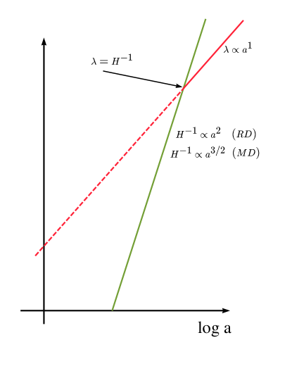
Figure 1: The horizon scale (solid line) and a physical scale $\lambda$ (dashed line) as function of the scale factor $a$

There were $\sim 10^{6}$ casually disconnected regions within the volume that now corresponds to our horizon! It is difficult to come up with a process other than an early hot and dense phase in the history of the universe that would lead to a precise black body for a bath of photons which were causally disconnected the last time they interacted with the surrounding plasma.

The horizon problem is well represented by Fig. 1 where the solid line indicates the horizon scale and the dashed line any generic physical length scale $\lambda$. Suppose, indeed, that $\lambda$ indicates the distance between two photons we detect today. From Eq. (17) we discover that at the time of emission (last-scattering) the two photons could not talk to each other, the dashed line is above the solid line [2]. [2]. There is another main point to mention with the horiton problem and it is related to the inhomogeneities. We know that the temperature anisotropy on the angular scale subtended by that length scale,

$$\left({\delta T\over T}\right)_{\theta}\approx\left({\delta\rho\over\rho}\right)_{\lambda},$$ (18)

where the scale $\lambda\sim 100h^{-1}\,{\rm Mpc}(\theta/{\rm deg})$ subtends an angle $\theta$ on the last-scattering surface. This is known as the Sachs–Wolfe effect [14, 15]. We shall come back to this piece of physics.

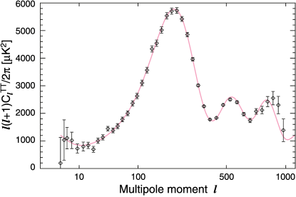
Figure 2: The CMBR anisotropy as function of $\ell$ (from Ref. [12])

The temperature anisotropy is commonly expanded in spherical harmonics

$$\frac{\Delta T}{T}(x_{0},\tau_{0},{\bf n})=\sum_{\ell m}a_{\ell,m}(x_{0})Y_{\ell m}({\bf n}),$$ (19)

where $x_{0}$ and $\tau_{0}$ are our position and the preset time, respectively, ${\bf n}$ is the direction of observation, $\ell^{\prime}$s are the different multipoles and

$$\langle a_{\ell m}a^{*}_{\ell^{\prime}m^{\prime}}\rangle=\delta_{\ell,\ell^{\prime}}\delta_{m,m^{\prime}}C_{\ell},$$ (20)

where the deltas are due to the fact that the process that created the anisotropy is statistically isotropic. The $C_{\ell}$’s are the so-called CMB power spectrum. For homogeneity and isotropy, the $C_{\ell}$’s are neither a function of $x_{0}$, nor of $m$. The two-point correlation function is related to the $C_{l}$’s in the following way

$$\Big{<}\frac{\delta T({\bf n})}{T}\frac{\delta T({\bf n}^{\prime})}{T}\Big{>} = \sum_{\ell\ell^{\prime}mm^{\prime}}\langle a_{\ell m}a^{*}_{\ell^{\prime}m^{\prime}}\rangle Y_{\ell m}({\bf n})Y^{*}_{\ell^{\prime}m^{\prime}}({\bf n}^{\prime})$$ (21)

$$= \sum_{\ell}C_{\ell}\sum_{m}Y_{\ell m}({\bf n})Y^{*}_{\ell m}({\bf n}^{\prime})=\frac{1}{4\pi}\sum_{\ell}(2\ell+1)C_{\ell}P_{\ell}(\mu={\bf n}\cdot{\bf n}^{\prime})$$

where we have used the addition theorem for the spherical harmonics, and $P_{\ell}$ is the Legendre polynom of order $\ell$. In expression (21) the expectation value is an ensemble average. It can be regarded as an average over the possible observer positions, but not in general as an average over the single sky we observe, because of the cosmic variance. WMAP5 data are given in Fig. 2.

Let us now consider the last scatteringsurface. In co-moving coordinates the latter is ‘far’ from us a distance equal to

$$\int_{t_{\rm LS}}^{t_{0}}\,\frac{dt}{a}=\int_{\tau_{\rm LS}}^{\tau_{0}}\,d\tau=\left(\tau_{0}-\tau_{\rm LS}\right).$$ (22)

A given co-moving scale $\lambda$ is therefore projected on the last scatteringsurface sky on an angular scale

$$\theta\simeq\frac{\lambda}{\left(\tau_{0}-\tau_{\rm LS}\right)},$$ (23)

where we have neglected tiny curvature effects. Consider now that the scale $\lambda$ is of the order of the co-moving sound horizon at the time of last-scattering, $\lambda\sim c_{s}\tau_{\rm LS}$, where $c_{s}\simeq 1/\sqrt{3}$ is the sound velocity at which photons propagate in the plasma at the last-scattering. This corresponds to an angle

$$\theta\simeq c_{s}\frac{\tau_{\rm LS}}{\left(\tau_{0}-\tau_{\rm LS}\right)}\simeq c_{s}\frac{\tau_{\rm LS}}{\tau_{0}},$$ (24)

where the last passage has been performed knowing that $\tau_{0}\gg\tau_{\rm LS}$. Since the universe is matter-dominated from the time of last scatteringonwards, the scale factor has the following behaviour: $a\sim T^{-1}\sim t^{2/3}\sim\tau^{2}$. The angle $\theta_{\rm HOR}$ subtended by the sound horizon on the last-scattering surface then becomes

$$\theta_{\rm HOR}\simeq c_{s}\left(\frac{T_{0}}{T_{\rm LS}}\right)^{1/2}\sim 1^{\circ},$$ (25)

where we have used $T_{\rm LS}\simeq 0.3$ eV and $T_{0}\sim 10^{-13}$ GeV. This corresponds to a multipole $\ell_{\rm HOR}$

$$\ell_{\rm HOR}=\frac{\pi}{\theta_{\rm HOR}}\simeq 200\,.$$ (26)

From these estimates we conclude that two photons which on the last scatteringsurface were separated by an angle larger than $\theta_{\rm HOR}$, corresponding to multipoles smaller than $\ell_{\rm HOR}\sim 200$, were not in causal contact. On the other hand, from Fig. 2 it is clear that small anisotropies, of the same order of magnitude $\delta T/T\sim 10^{-5}$ are present at $\ell\ll 200$. We conclude that one of the striking features of the CMB fluctuations is that they appear to be non-causal.

As can be seen in Fig. 1, in the standard cosmology the physical size of a perturbation, which grows as the scale factor, begins larger than the horizon and, relatively late in the history of the universe, crosses inside the horizon. This precludes a causal microphysical explanation for the origin of the required density perturbations.

From the considerations made so far, it appears that solving the horizon problem of the standard Big Bang theory requires that the universe go through a primordial period during which the physical scales $\lambda$ evolve faster than the horizon scale $H^{-1}$.

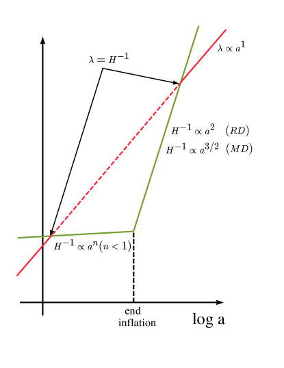
Figure 3: The behaviour of a generic scale $\lambda$ and the horizon scale $H^{-1}$ in the standard inflationary model

If there is period during which physical length scales grow faster than $H^{-1}$, length scales $\lambda$ which are within the horizon today, $\lambda<H^{-1}$ (such as the distance between two detected photons) and were outside the horizon for some period, $\lambda>H^{-1}$ (for instance at the time of last scatteringwhen the two photons were emitted), had a chance to be within the horizon at some primordial epoch, $\lambda<H^{-1}$ again, see Fig. 3. If this happens, the homogeneity and the isotropy of the CMB can easily be explained: photons that we receive today and were emitted from the last scattering surface from causally disconnected regions have the same temperature because they had a chance to ‘talk’ to each other at some primordial stage of the evolution of the universe.

The second condition can easily be expressed as a condition on the scale factor $a$. Since a given scale $\lambda$ scales like $\lambda\sim a$ and $H^{-1}=a/\dot{a}$, we need to impose that there is a period during which

$$\left(\frac{\lambda}{H^{-1}}\right)^{\cdot}=\ddot{a}>0\,.$$

We can therefore introduce the following rigorous definition: an inflationary stage is a period of the universe during which the latter accelerates

INFLATION   ⟺   ¨a>0.

Comment: Let us stress that during such an accelerating phase the universe expands adiabatically. This means that during inflation one can exploit the usual FRW equations (3) and (5). It must be clear therefore that the non-adiabaticity condition is satisfied not during inflation, but during the phase transition between the end of inflation and the beginning of the radiation-dominated phase. At this transition phase a large entropy is generated under the form of relativistic degrees of freedom: the Big Bang has taken place.

0.4 The standard inflationary universe

Some parts which follow are taken from [3] and [5]. We thank E.W. Kolb fand A. Linde or granting permission. From the previous section we have learned that an accelerating stage during the primordial phases of the evolution of the universe might be able to solve the horizon problem. From Eq. (5) we learn that

$$\ddot{a}>0\Longleftrightarrow(\rho+3P)<0\,.$$

An accelerating period is obtainable only if the overall pressure $p$ of the universe is negative: $p<-\rho/3$. Neither a radiation-dominated phase nor a matter-dominated phase (for which $p=\rho/3$ and $p=0$, respectively) satisfy such a condition. Let us postpone for the time being the problem of finding a ‘candidate’ able to provide the condition $P<-\rho/3$. For sure, inflation is a phase of the history of the universe occurring before the era of nucleosynthesis ($t\approx 1$ s, $T\approx 1$ MeV) during which the light elements abundances were formed. This is because nucleosynthesis is the earliest epoch from which we have experimental data and they are in agreement with the predictions of the standard Big Bang theory. However, the thermal history of the universe before the epoch of nucleosynthesis is unknown.

In order to study the properties of the period of inflation, we assume the extreme condition $p=-\rho$ which considerably simplifies the analysis. A period of the universe during which $P=-\rho$ is called the de Sitter stage. By inspecting Eqs. (3) and (4), we learn that during the de Sitter phase

$$\rho = \leavevmode\nobreak\ \leavevmode\nobreak\ {\rm constant}\,,$$

$$H_{I} = \leavevmode\nobreak\ \leavevmode\nobreak\ {\rm constant}\,,$$

where we have indicated by $H_{I}$ the value of the Hubble rate during inflation. Correspondingly, solving Eq. (3) gives

$$a=a_{i}\,e^{H_{I}(t-t_{i})},$$ (27)

where $t_{i}$ denotes the time at which inflation starts. Let us now see how such a period of exponential expansion takes care of the shortcomings of the standard Big Bang Theory.

0.4.1 Inflation and the horizon problem

During the inflationary (de Sitter) epoch the horizon scale $H^{-1}$ is constant. If inflation lasts long enough, all the physical scales that have left the horizon during the radiation-dominated or matter-dominated phase can re-enter the horizon in the past: this is because such scales are exponentially reduced. As we have seen in the previous section, this explains both the problem of the homogeneity of CMB and the initial condition problem of small cosmological perturbations. Once the physical length is within the horizon, microphysics can act, the universe can be made approximately homogeneous and the primeval inhomogeneities can be created.

Let us see how long inflation must be sustained in order to solve the horizon problem. Let $t_{i}$ and $t_{f}$ be, respectively, the time of beginning and end of inflation. We can define the corresponding number of e-foldings $N$

$$N={\rm ln}\left[H_{I}(t_{e}-t_{i})\right].$$ (28)

A necessary condition to solve the horizon problem is that the largest scale we observe today, the present horizon $H_{0}^{-1}$, was reduced during inflation to a value $\lambda_{H_{0}}(t_{i})$ smaller than the value of horizon length $H_{I}^{-1}$ during inflation. This gives

$$\lambda_{H_{0}}(t_{i})=H^{-1}_{0}\left(\frac{a_{t_{f}}}{a_{t_{0}}}\right)\left(\frac{a_{t_{i}}}{a_{t_{f}}}\right)=H_{0}^{-1}\left(\frac{T_{0}}{T_{f}}\right)e^{-N}\mathrel{\mathchoice{\lower 3.6pt\vbox{\halign{$\mathsurround=0pt\displaystyle\hfil#\hfil$\cr<\crcr\sim\crcr}}}{\lower 3.6pt\vbox{\halign{$\mathsurround=0pt\textstyle\hfil#\hfil$\cr<\crcr\sim\crcr}}}{\lower 3.6pt\vbox{\halign{$\mathsurround=0pt\scriptstyle\hfil#\hfil$\cr<\crcr\sim\crcr}}}{\lower 3.6pt\vbox{\halign{$\mathsurround=0pt\scriptscriptstyle\hfil#\hfil$\cr<\crcr\sim\crcr}}}}H_{I}^{-1},$$

where we have neglected for simplicity the short period of matter-domination and we have called $T_{f}$ the temperature at the end of inflation (to be indentified with the reheating temperature $T_{RH}$ at the beginning of the radiation-dominated phase after inflation, see later). We get

$$N\mathrel{\mathchoice{\lower 3.6pt\vbox{\halign{$\mathsurround=0pt\displaystyle\hfil#\hfil$\cr>\crcr\sim\crcr}}}{\lower 3.6pt\vbox{\halign{$\mathsurround=0pt\textstyle\hfil#\hfil$\cr>\crcr\sim\crcr}}}{\lower 3.6pt\vbox{\halign{$\mathsurround=0pt\scriptstyle\hfil#\hfil$\cr>\crcr\sim\crcr}}}{\lower 3.6pt\vbox{\halign{$\mathsurround=0pt\scriptscriptstyle\hfil#\hfil$\cr>\crcr\sim\crcr}}}}\ln\left(\frac{T_{0}}{H_{0}}\right)-\ln\left(\frac{T_{f}}{H_{I}}\right)\approx 67+\ln\left(\frac{T_{f}}{H_{I}}\right).$$

Apart from the logarithmic dependence, we obtain $N\mathrel{\mathchoice{\lower 3.6pt\vbox{\halign{$\mathsurround=0pt\displaystyle\hfil#\hfil$\cr>\crcr\sim\crcr}}}{\lower 3.6pt\vbox{\halign{$\mathsurround=0pt\textstyle\hfil#\hfil$\cr>\crcr\sim\crcr}}}{\lower 3.6pt\vbox{\halign{$\mathsurround=0pt\scriptstyle\hfil#\hfil$\cr>\crcr\sim\crcr}}}{\lower 3.6pt\vbox{\halign{$\mathsurround=0pt\scriptscriptstyle\hfil#\hfil$\cr>\crcr\sim\crcr}}}}70$.

0.4.2 A prediction of inflation

Since during inflation the Hubble rate is constant

$$\Omega-1=\frac{k}{a^{2}H^{2}}\propto\frac{1}{a^{2}}\ .$$

On the other hand it is easy to show that to reproduce a value of $(\Omega_{0}-1)$ of order of unity today, the initial value of $(\Omega-1)$ at the beginning of the radiation-dominated phase must be $\left|\Omega-1\right|\sim 10^{-60}$. Since we identify the beginning of the radiation-dominated phase with the beginning of inflation, we require

$$\left|\Omega-1\right|_{t=t_{f}}\sim 10^{-60}.$$

During inflation

$$\frac{\left|\Omega-1\right|_{t=t_{f}}}{\left|\Omega-1\right|_{t=t_{i}}}=\left(\frac{a_{i}}{a_{f}}\right)^{2}=e^{-2N}.$$ (29)

Taking $\left|\Omega-1\right|_{t=t_{i}}$ of order unity, it is enough to require that $N\approx 70$. However, IF the period of inflation lasts longer than 70 e-foldings the present-day value of $\Omega_{0}$ will be equal to unity with great precision. One can say that a generic prediction of inflation is that

INFLATION   ⟹   Ω_0=1.

This statement, however, must be taken cum grano salis and properly specified. Inflation does not change the global geometric properties of the space-time. If the universe is open or closed, it will always remain flat or closed, independently from inflation. What inflation does is to magnify the radius of curvature $R_{\rm curv}$ defined in Eq. (9) so that locally the universe is flat with a great precision. As we shall see, the current data on the CMB anisotropies confirm this prediction.

0.4.3 Inflation and the inflaton

In the previous subsections we have described the various advantages of having a period of accelerating phase. The latter required $P<-\rho/3$. Now, we would like to show that this condition can be attained by means of a simple scalar field. We shall call this field the inflaton $\phi$.

The action of the inflaton field reads

$$S=\int d^{4}x\,\sqrt{-g}\,\mathcal{L}=\int\,d^{4}x\,\sqrt{-g}\,\left[\frac{1}{2}\partial_{\mu}\phi\partial^{\mu}\phi+V(\phi)\right],$$ (30)

where $\sqrt{-g}=a^{3}$ for the FRW metric (1). From the Euler–Lagrange equations

$$\partial^{\mu}\frac{\delta(\sqrt{-g}\mathcal{L})}{\delta\,\partial^{\mu}\phi}-\frac{\delta(\sqrt{-g}\mathcal{L})}{\delta\phi}=0\,,$$ (31)

we obtain

$$\ddot{\phi}+3H\dot{\phi}-\frac{\nabla^{2}\phi}{a^{2}}+V^{\prime}(\phi)=0\,,$$ (32)

where $V^{\prime}(\phi)=\left(dV(\phi)/d\phi\right)$. Note, in particular, the appearance of the friction term $3H\dot{\phi}$: a scalar field rolling down its potential suffers a friction due to the expansion of the universe.

We can write the energy momentum tensor of the scalar field

$$T_{\mu\nu}=\partial_{\mu}\phi\partial_{\nu}\phi-g_{\mu\nu}\,\mathcal{L}\,.$$

The corresponding energy density $\rho_{\phi}$ and pressure density $P_{\phi}$ are

$$T_{00}=\rho_{\phi}=\frac{\dot{\phi}^{2}}{2}+V(\phi)+\frac{(\nabla\phi)^{2}}{2a^{2}},$$ (33)

$$T_{ii}=P_{\phi}=\frac{\dot{\phi}^{2}}{2}-V(\phi)-\frac{(\nabla\phi)^{2}}{6a^{2}}\,.$$ (34)

Note that, if the gradient term were dominant, we would obtain $P_{\phi}=-\frac{\rho_{\phi}}{3}$, not enough to drive inflation. We can now split the inflaton field in

$$\phi(t)=\phi_{0}(t)+\delta\phi({\bf x},t)\,,$$

where $\phi_{0}$ is the ‘classical’ (infinite wavelength) field, that is the expectation value of the inflaton field on the initial isotropic and homogeneous state, while $\delta\phi({\bf x},t)$ represents the quantum fluctuations around $\phi_{0}$. In this section, we shall be concerned only with the evolution of the classical field $\phi_{0}$. The next section will be devoted to the crucial issue of the evolution of quantum perturbations during inflation. This separation is justified by the fact that quantum fluctuations are much smaller than the classical value and therefore negligible when looking at the classical evolution. Not to be overwhelmed by the notation, we shall indicate the classical value of the inflaton field by $\phi$ from now on. The energy momentum tensor becomes

$$T_{00}=\rho_{\phi}=\frac{\dot{\phi}^{2}}{2}+V(\phi)$$ (35)

$$T_{ii}=P_{\phi}=\frac{\dot{\phi}^{2}}{2}-V(\phi).$$ (36)

If

$$V(\phi)\gg\dot{\phi}^{2}$$

we obtain the following condition

$$P_{\phi}\simeq-\rho_{\phi}\,.$$

From this simple calculation, we realize that a scalar field whose energy is dominant in the universe and whose potential energy dominates over the kinetic term gives inflation. Inflation is driven by the vacuum energy of the inflaton field.

0.4.4 Slow-roll conditions

Let us now quantify better under which circumstances a scalar field may give rise to a period of inflation. The equation of motion of the field is

$$\ddot{\phi}+3H\dot{\phi}+V^{\prime}(\phi)=0\,.$$ (37)

If we require that $\dot{\phi}^{2}\ll V(\phi)$, the scalar field is slowly rolling down its potential. This is the reason why such a period is called slow-roll. We may also expect that since the potential is flat, $\ddot{\phi}$ is negligible as well. We shall assume that this is true and we shall quantify this condition soon. The FRW equation (3) becomes

$$H^{2}\simeq\frac{8\pi G}{3}\,V(\phi),$$ (38)

where we have assumed that the inflaton field dominates the energy density of the universe. The new equation of motion becomes

$$3H\dot{\phi}=-V^{\prime}(\phi)$$ (39)

which gives $\dot{\phi}$ as a function of $V^{\prime}(\phi)$. Using Eq. (39) slow-roll conditions then require

$$\dot{\phi}^{2}\ll V(\phi)\\ \Longrightarrow\\ \frac{(V^{\prime})^{2}}{V}\ll H^{2}$$

and

$$\ddot{\phi}\ll 3H\dot{\phi}\\ \Longrightarrow\\ V^{\prime\prime}\ll H^{2}.$$

It is now useful to define the slow-roll parameters $\epsilon$ and $\eta$ in the following way

$\displaystyle\epsilon$ $\displaystyle=$ $\displaystyle-\frac{\dot{H}}{H^{2}}=4\pi G\frac{\dot{\phi}^{2}}{H^{2}}=\frac{1}{16\pi G}\left(\frac{V^{\prime}}{V}\right)^{2},$ $\displaystyle\eta$ $\displaystyle=$ $\displaystyle\frac{1}{8\pi G}\left(\frac{V^{\prime\prime}}{V}\right)=\frac{1}{3}\frac{V^{\prime\prime}}{H^{2}},$ $\displaystyle\delta$ $\displaystyle=$ $\displaystyle\eta-\epsilon=-\frac{\ddot{\phi}}{H\dot{\phi}}\,.$

It might be useful to have the same parameters expressed in terms of conformal time

$\displaystyle\epsilon$ $\displaystyle=$ $\displaystyle 1-\frac{\,{\cal H}^{\prime}}{\,{\cal H}^{2}}=4\pi G\frac{\phi{{}^{\prime}}^{2}}{\,{\cal H}^{2}}$ $\displaystyle\delta$ $\displaystyle=$ $\displaystyle\eta-\epsilon=1-\frac{\phi^{\prime\prime}}{\,{\cal H}\phi^{\prime}}\,.$

The parameter $\epsilon$ quantifies how much the Hubble rate $H$ changes with time during inflation. Notice that, since

$$\frac{\ddot{a}}{a}=\dot{H}+H^{2}=\left(1-\epsilon\right)H^{2},$$

inflation can be attained only if $\epsilon<1$:

INFLATION   ⟺   ϵ<1.

As soon as this condition fails, inflation ends. In general, slow-roll inflation is attained if $\epsilon\ll 1$ and $|\eta|\ll 1$. During inflation the slow-roll parameters $\epsilon$ and $\eta$ can be considered to be approximately constant since the potential $V(\phi)$ is very flat.

Comment: In the following, we shall work at first-order perturbation in the slow-roll parameters, that is we shall take only the first power of them. Since, using their definition, it is easy to see that $\dot{\epsilon},\dot{\eta}={\cal O}\left(\epsilon^{2},\eta^{2}\right)$, this amounts to saying that we shall treat the slow-roll parameters as constant in time.

Within these approximations, it is easy to compute the number of e-foldings between the beginning and the end of inflation. If we indicate by $\phi_{i}$ and $\phi_{f}$ the values of the inflaton field at the beginning and at the end of inflation, respectively, we find that the total number of e-foldings is

$$N \equiv \int_{t_{i}}^{t_{f}}\,H\,dt$$ (40)

$$\simeq H\int^{\phi_{f}}_{\phi_{i}}\frac{d\phi}{\dot{\phi}}$$

$$\simeq -3H^{2}\int^{\phi_{f}}_{\phi_{i}}\frac{d\phi}{V^{\prime}}$$

$$\simeq -8\pi G\int^{\phi_{f}}_{\phi_{i}}\frac{V}{V^{\prime}}\,d\phi\,.$$

We may also compute the number of e-foldings $\Delta N$ which are left to go to the end of inflation

$$\Delta N\simeq 8\pi G\int^{\phi_{\Delta N}}_{\phi_{f}}\frac{V}{V^{\prime}}\,d\phi,$$ (41)

where $\phi_{\Delta N}$ is the value of the inflaton field when there are $\Delta N$ e-foldings to the end of inflation.

1. Comment: According to the criterion given in Subsection 2.4, a given scale length $\lambda=a/k$ leaves the horizon when $k=aH_{k}$ where $H_{k}$ is the the value of the Hubble rate at that time. One can easily compute the rate of change of $H^{2}_{k}$ as a function of $k$

$$\frac{d{\rm ln}\,H_{k}^{2}}{d{\rm ln}\,k}=\left(\frac{d{\rm ln}\,H_{k}^{2}}{dt}\right)\left(\frac{dt}{d{\rm ln}\,a}\right)\left(\frac{d{\rm ln}\,a}{d{\rm ln}\,k}\right)=2\frac{\dot{H}}{H}\times\frac{1}{H}\times 1=2\frac{\dot{H}}{H^{2}}=-2\epsilon.$$ (42)

2. Comment: Take a given physical scale $\lambda$ today which crossed the horizon scale during inflation. This happened when

$$\lambda\left(\frac{a_{f}}{a_{0}}\right)e^{-\Delta N_{\lambda}}=\lambda\left(\frac{T_{0}}{T_{f}}\right)e^{-\Delta N_{\lambda}}=H_{I}^{-1}$$

where $\Delta N_{\lambda}$ indicates the number of e-foldings from the time the scale crossed the horizon during inflation and the end of inflation. This relation gives a way to determine the number of e-foldings to the end of inflation corresponding to a given scale

$$\Delta N_{\lambda}\simeq 65+{\rm ln}\left(\frac{\lambda}{3000\,\,{\rm Mpc}}\right)+2\,{\rm ln}\left(\frac{V^{1/4}}{10^{14}\,\,{\rm GeV}}\right)-{\rm ln}\left(\frac{T_{f}}{10^{10}\,\,{\rm GeV}}\right).$$

Scales relevant for the CMB anisotropies correspond to $\Delta N\sim$60.

Inflation ended when the potential energy associated with the inflaton field became smaller than the kinetic energy of the field. By that time, any pre-inflation entropy in the universe had been inflated away, and the energy of the universe was entirely in the form of coherent oscillations of the inflaton condensate around the minimum of its potential. The universe may be said to be frozen after the end of inflation. We know that somehow the low-entropy cold universe dominated by the energy of coherent motion of the $\phi$ field must be transformed into a high-entropy hot universe dominated by radiation. The process by which the energy of the inflaton field is transferred from the inflaton field to radiation has been dubbed reheating. In the theory of reheating, the simplest way to envisage this process is if the co-moving energy density in the zero mode of the inflaton decays into normal particles, which then scatter and thermalize to form a thermal background. It is usually assumed that the decay width of this process is the same as the decay width of a free inflaton field.

Of particular interest is a quantity usually known as the reheat temperature, denoted as $T_{RH}$. The reheat temperature is calculated by assuming an instantaneous conversion of the energy density in the inflaton field into radiation when the decay width of the inflaton energy, $\Gamma_{\phi}$, is equal to $H$, the expansion rate of the universe.

The reheat temperature is calculated quite easily. After inflation the inflaton field executes coherent oscillations about the minimum of the potential. Averaged over several oscillations, the coherent oscillation energy density redshifts as matter: $\rho_{\phi}\propto a^{-3}$, where $a$ is the Robertson–Walker scale factor. If we denote as $\rho_{I}$ and $a_{I}$ the total inflaton energy density and the scale factor at the initiation of coherent oscillations, then the Hubble expansion rate as a function of $a$ is

$$H^{2}(a)=\frac{8\pi}{3}\frac{\rho_{I}}{{m_{\rm Pl}}^{2}}\left(\frac{a_{I}}{a}\right)^{3}.$$ (43)

Equating $H(a)$ and $\Gamma_{\phi}$ leads to an expression for $a_{I}/a$. Now if we assume that all available coherent energy density is instantaneously converted into radiation at this value of $a_{I}/a$, we can find the reheat temperature by setting the coherent energy density, $\rho_{\phi}=\rho_{I}(a_{I}/a)^{3}$, equal to the radiation energy density, $\rho_{R}=(\pi^{2}/30)g_{*}T_{RH}^{4}$, where $g_{*}$ is the effective number of relativistic degrees of freedom at temperature $T_{RH}$. The result is

$$T_{RH}=\left(\frac{90}{8\pi^{3}g_{*}}\right)^{1/4}\sqrt{\Gamma_{\phi}{m_{\rm Pl}}}\ =0.2\left(\frac{200}{g_{*}}\right)^{1/4}\sqrt{\Gamma_{\phi}{m_{\rm Pl}}}\ .$$ (44)

0.5 Inflation and the cosmological perturbations

In order for structure formation to occur via gravitational instability, there must have been small pre-existing fluctuations on physical length scales when they crossed the Hubble radius in the radiation-dominated and matter-dominated eras [7]. These fluctuations are given by inflation. Indeed, In an exponentially expanding universe the wavelenghts of all vacuum fluctuations of the inflaton field $\phi$ grow exponentially in the expanding universe. When the wavelength of any particular fluctuation becomes greater than $H^{-1}$, this fluctuation stops propagating, and its amplitude freezes at some non-zero value $\delta\phi$ because of the large friction term $3H\dot{\phi}$ the equation of motion of the field $\phi$. The amplitude of this fluctuation then remains almost unchanged for a very long time, whereas its wavelength grows exponentially to cosmological scales.

Once inflation has ended, however, the Hubble radius increases faster than the scale factor, so the fluctuations eventually re-enter the Hubble radius during the radiation- or matter-dominated eras and provide the necessary seeds.

In summary, these are the key ingredients for understanding the observed structures in the universe within the inflationary scenario:

• Quantum fluctuations of the inflaton field are excited during inflation and stretched to cosmological scales. At the same time, being the inflaton fluctuations connected to the metric perturbations through Einstein’s equations, ripples on the metric are also excited and stretched to cosmological scales.

• Gravity acts a messenger since it communicates the small seed perturbations to photons and baryons once a given wavelength becomes smaller than the horizon scale after inflation.

Let us now see how quantum fluctuations are generated during inflation. we shall proceed by steps. First, we shall consider the simplest problem of studying the quantum fluctuations of a generic scalar field during inflation: we shall learn how perturbations evolve as a function of time and compute their spectrum. Then—since a satisfactory description of the generation of quantum fluctuations has to take both the inflaton and the metric perturbations into account— we shall study the system composed by quantum fluctuations of the inflaton field and quantum fluctuations of the metric.

0.6 Quantum fluctuations of a generic massless scalar field during inflation

Let us first see how the fluctuations of a generic scalar field $\chi$, which is not the inflaton field, behave during inflation. To warm up we first consider a de Sitter epoch during which the Hubble rate is constant.

0.6.1 Quantum fluctuations of a generic massless scalar field during a de Sitter stage

We assume this field to be massless. The massive case will be analysed in the next subsection.

Expanding the scalar field $\chi$ in Fourier modes

$$\delta\chi({\bf x},t)=\int\,\frac{d^{3}{\bf k}}{(2\pi)^{3/2}}\,e^{i{\bf k}\cdot{\bf x}}\,\delta\chi_{{\bf k}}(t),$$

we can write the equation for the fluctuations as

$$\delta\ddot{\chi}_{\bf k}+3H\,\delta\dot{\chi}_{\bf k}+\frac{k^{2}}{a^{2}}\,\delta\chi_{\bf k}=0\,.$$ (45)

Let us study the qualitative behaviour of the solution to Eq. (45).

• For wavelengths within the horizon, $\lambda\ll H^{-1}$, the corresponding wave-number satisfies the relation $k\gg a\,H$. In this regime, we can neglect the friction term $3H\,\delta\dot{\chi}_{\bf k}$ and Eq. (45) reduces to

  $$\delta\ddot{\chi}_{\bf k}+\frac{k^{2}}{a^{2}}\,\delta\chi_{\bf k}=0,$$ (46)

  which is basically the equation of motion of an harmonic oscillator. Of course, the frequency term $k^{2}/a^{2}$ depends upon time because the scale factor $a$ grows exponentially. On the qualitative level, however, one expects that when the wavelength of the fluctuation is within the horizon, the fluctuation oscillates.

• For wavelengths above the horizon, $\lambda\gg H^{-1}$, the corresponding wave-number satisfies the relation $k\ll aH$ and the term $k^{2}/a^{2}$ can be safely neglected. Equation (45) reduces to

  $$\delta\ddot{\chi}_{\bf k}+3H\,\delta\dot{\chi}_{\bf k}=0,$$ (47)

  which tells us that on superhorizon scales $\delta\chi_{\bf k}$ remains constant.

We have therefore the following picture: take a given fluctuation whose initial wavelength $\lambda\sim a/k$ is within the horizon. The fluctuations oscillate till the wavelength becomes of the order of the horizon scale. When the wavelength crosses the horizon, the fluctuation ceases to oscillate and gets frozen in.

Let us now study the evolution of the fluctuation in a more quantitative way. To do so, we perform the following redefinition

$$\delta\chi_{\bf k}=\frac{\delta\sigma_{\bf k}}{a}$$

and we work in conformal time $d\tau=dt/a$. For the time being, we solve the problem for a pure de Sitter expansion and we take the scale factor exponentially growing as $a\sim e^{Ht}$; the corresponding conformal factor reads (after choosing properly the integration constants)

$$a(\tau)=-\frac{1}{H\tau}\,\,\,\,(\tau<0).$$

In the following we shall also solve the problem in the case of quasi de Sitter expansion. The beginning of inflation coincides with some initial time $\tau_{i}\ll 0$. We find that Eq. (45) becomes

$$\delta\sigma^{\prime\prime}_{\bf k}+\left(k^{2}-\frac{a^{\prime\prime}}{a}\right)\delta\sigma_{\bf k}=0.$$ (48)

We obtain an equation which is very ‘close’ to the equation for a Klein–Gordon scalar field in flat space-time, the only difference being a negative time-dependent mass term $-a^{\prime\prime}/a=-2/\tau^{2}$. Equation (48) can be obtained from an action of the type

$$\delta S_{\bf k}=\int\,d\tau\,\left[\frac{1}{2}\delta\sigma^{\prime 2}_{\bf k}-\frac{1}{2}\left(k^{2}-\frac{a^{\prime\prime}}{a}\right)\delta\sigma^{2}_{\bf k}\right],$$ (49)

which is the canonical action for a simple harmonic oscillator with canonical commutation relations $\delta\sigma^{*}_{\bf k}\delta\sigma^{\prime}_{\bf k}-\delta\sigma_{\bf k}\delta\sigma^{*\prime}_{\bf k}=-i$.

Let us study the behaviour of this equation on subhorizon and superhorizon scales. Since

$$\frac{k}{aH}=-k\,\tau\,,$$

on subhorizon scales $k^{2}\gg a^{\prime\prime}/a$ Equation (48) reduces to

$$\delta\sigma^{\prime\prime}_{\bf k}+k^{2}\,\delta\sigma_{\bf k}=0\,,$$

whose solution is a plane wave

$$\delta\sigma_{\bf k}=\frac{e^{-ik\tau}}{\sqrt{2k}}\,\,\,\,(k\gg aH)\,.$$ (50)

We find again that fluctuations with wavelength within the horizon oscillate exactly like in flat space-time. This does not come as a surprise. In the ultraviolet regime, that is for wavelengths much smaller than the horizon scale, one expects that approximating the space-time as flat is a good approximation.

On superhorizon scales, $k^{2}\ll a^{\prime\prime}/a$ Equation (48) reduces to

$$\delta\sigma^{\prime\prime}_{\bf k}-\frac{a^{\prime\prime}}{a}\delta\sigma_{\bf k}=0,$$

which is satisfied by

$$\delta\sigma_{\bf k}=B(k)\,a\,\,\,\,(k\ll aH)\,$$ (51)

where $B(k)$ is a constant of integration. Roughly matching the (absolute values of the) solutions $(\ref{q1})$ and $(\ref{x2})$ at $k=aH$ ($-k\tau=1$), we can determine the (absolute value of the) constant $B(k)$

$$\left|B(k)\right|a=\frac{1}{\sqrt{2k}}\Longrightarrow\left|B(k)\right|=\frac{1}{a\sqrt{2k}}=\frac{H}{\sqrt{2k^{3}}}.$$

Going back to the original variable $\delta\chi_{\bf k}$, we obtain that the quantum fluctuation of the $\chi$ field on superhorizon scales is constant and approximately equal to

|δχ_k|≃H2k3     (ON  SUPERHORIZON  SCALES)

In fact we can do much better, since Eq. (48) has an exact solution:

$$\delta\sigma_{\bf k}=\frac{e^{-ik\tau}}{\sqrt{2k}}\left(1+\frac{i}{k\tau}\right).$$ (52)

This solution reproduces all that we have found by qualitative arguments in the two extreme regimes $k\ll aH$ and $k\gg aH$. We have performed the matching procedure to show that the latter can be very useful to determine the behaviour of the solution on superhorizon scales when the exact solution is not known.

0.6.2 The power spectrum

Let us define now the power spectrum, a useful quantity to characterize the properties of the perturbations. For a generic quantity $g({\bf x},t)$, which can expanded in Fourier space as

$$g({\bf x},t)=\int\,\frac{d^{3}{\bf k}}{(2\pi)^{3/2}}\,e^{i{\bf k}\cdot{\bf x}}\,g_{{\bf k}}(t),$$

the power spectrum can be defined as

$$\langle 0|g^{*}_{{\bf k}_{1}}g_{{\bf k}_{2}}|0\rangle\equiv\delta^{(3)}\left({\bf k}_{1}-{\bf k}_{2}\right)\,\frac{2\pi^{2}}{k^{3}}\,{\cal P}_{g}(k),$$ (53)

where $\left|0\right.\rangle$ is the vacuum quantum state of the system. This definition leads to the usual relation

$$\langle 0|g^{2}({\bf x},t)|0\rangle=\int\,\frac{dk}{k}\,{\cal P}_{g}(k).$$ (54)

0.6.3 Quantum fluctuations of a generic scalar field in a quasi de Sitter stage

So far, we have computed the time evolution and the spectrum of the quantum fluctuations of a generic scalar field $\chi$ supposing that the scale factor evolves like in a pure de Sitter expansion, $a(\tau)=-1/(H\tau)$. However, during inflation the Hubble rate is not exactly constant, but changes with time as $\dot{H}=-\epsilon\,H^{2}$ (quasi de Sitter expansion). In this subsection, we shall solve for the perturbations in a quasi de Sitter expansion. Using the definition of the conformal time, one can show that the scale factor for small values of $\epsilon$ becomes

$$a(\tau)=-\frac{1}{H}\frac{1}{\tau(1-\epsilon)}.$$

The fluctuation mass-squared mass term is

$$M^{2}(\tau)=m_{\chi}^{2}a^{2}-\frac{a^{\prime\prime}}{a},$$

where

$$\frac{a^{\prime\prime}}{a} = a^{2}\left(\frac{\ddot{a}}{a}+H^{2}\right)=a^{2}\left(\dot{H}+2\,H^{2}\right)$$ (55)

$$= a^{2}\left(2-\epsilon\right)H^{2}=\frac{\left(2-\epsilon\right)}{\tau^{2}\left(1-\epsilon\right)^{2}}$$

$$\simeq \frac{1}{\tau^{2}}\left(2+3\epsilon\right).$$

Armed with these results, we may compute the variance of the perturbations of the generic $\chi$ field

$$\langle 0|\left(\delta\chi({\bf x},t)\right)^{2}|0\rangle = \int\,\frac{d^{3}k}{(2\pi)^{3}}\,\left|\delta\chi_{\bf k}\right|^{2}$$ (56)

$$= \int\,\frac{dk}{k}\,\frac{k^{3}}{2\pi^{2}}\,\left|\delta\chi_{\bf k}\right|^{2}$$

$$= \int\,\frac{dk}{k}\,{\cal P}_{\delta\chi}(k),$$

which defines the power spectrum of the fluctuations of the scalar field $\chi$

$${\cal P}_{\delta\chi}(k)\equiv\frac{k^{3}}{2\pi^{2}}\,\left|\delta\chi_{\bf k}\right|^{2}.$$ (57)

Since we have seen that fluctuations are (nearly) frozen in on superhorizon scales, a way of characterizing the perturbations is to compute the spectrum on scales larger than the horizon. For a massive scalar field, we obtain

$${\cal P}_{\delta\chi}(k)=\left(\frac{H}{2\pi}\right)^{2}\left(\frac{k}{aH}\right)^{3-2\nu_{\chi}},$$ (58)

where, taking $m_{\chi}^{2}/H^{2}=3\eta_{\chi}$ and expanding for small values of $\epsilon$ and $\eta$,

$$\nu_{\chi}\simeq\frac{3}{2}+\epsilon-\eta_{\chi}.$$ (59)

We may also define the spectral index $n_{\delta\chi}$ of the fluctuations as

n_δχ-1= d ln  Pδϕd ln  k=3-2ν_χ= 2η_χ-2ϵ.

The power spectrum of fluctuations of the scalar field $\chi$ is therefore nearly flat, that is is nearly independent of the wavelength $\lambda=\pi/k$: the amplitude of the fluctuation on superhorizon scales does almost not depend upon the time at which the fluctuation crosses the horizon and becomes frozen in. The small tilt of the power spectrum arises from the fact that the scalar field $\chi$ is massive and because during inflation the Hubble rate is not exactly constant, but nearly constant, where ‘nearly’ is quantified by the slow-roll parameters $\epsilon$. Adopting the traditional terminology, we may say that the spectrum of perturbations is blue if $n_{\delta\chi}>1$ (more power in the ultraviolet) and red if $n_{\delta\chi}<1$ (more power in the infrared). The power spectrum of the perturbations of a generic scalar field $\chi$ generated during a period of slow-roll inflation may be either blue or red. This depends upon the relative magnitude between $\eta_{\chi}$ and $\epsilon$.

Comment: We might have computed the spectral index of the spectrum ${\cal P}_{\delta\chi}(k)$ by first solving the equation for the perturbations of the field $\chi$ in a di Sitter stage, with $H=$ constant and therefore $\epsilon=0$, and then taking into account the time evolution of the Hubble rate introducing the subscript in $H_{k}$ whose time variation is determined by Eq. (42). Correspondingly, $H_{k}$ is the value of the Hubble rate when a given wavelength $\sim k^{-1}$ crosses the horizon (from that point on the fluctuation remains frozen in). The power spectrum in such an approach would read

$${\cal P}_{\delta\chi}(k)=\left(\frac{H_{k}}{2\pi}\right)^{2}\left(\frac{k}{aH}\right)^{3-2\nu_{\chi}}$$ (60)

with $3-2\nu_{\chi}\simeq\eta_{\chi}$. Using Eq. (42), one finds

$$n_{\delta\chi}-1=\frac{d{\rm ln}\,{\cal P}_{\delta\phi}}{d{\rm ln}\,k}=\frac{d{\rm ln}\,H_{k}^{2}}{d{\rm ln}\,k}+3-2\nu_{\chi}=2\eta_{\chi}-2\epsilon$$

which reproduces our previous findings.

Comment: Since on superhorizon scales

$$\delta\chi_{\bf k}\simeq\frac{H}{\sqrt{2k^{3}}}\left(\frac{k}{aH}\right)^{\eta_{\chi}-\epsilon}\simeq\frac{H}{\sqrt{2k^{3}}}\left[1+\left(\eta_{\chi}-\epsilon\right){\rm ln}\,\left(\frac{k}{aH}\right)\right],$$

we discover that

$$\left|\delta\dot{\chi}_{\bf k}\right|\simeq\left|H\left(\eta_{\chi}-\epsilon\right)\,\delta\chi_{\bf k}\right|\ll\left|H\,\delta\chi_{\bf k}\right|,$$ (61)

that is, on superhorizon scales the time variation of the perturbations can be safely neglected.

0.7 Quantum fluctuations during inflation

As we have mentioned in the previous section, the linear theory of the cosmological perturbations represents a cornerstone of modern cosmology and is used to describe the formation and evolution of structures in the universe as well as the anisotropies of the CMB. The seeds for these inhomogeneities were generated during inflation and stretched over astronomical scales because of the rapid superluminal expansion of the universe during the (quasi) de Sitter epoch.

In the previous section we have already seen that pertubations of a generic scalar field $\chi$ are generated during a (quasi) de Sitter expansion. The inflaton field is a scalar field and, as such, we conclude that inflaton fluctuations will be generated as well. However, the inflaton is special from the point of view of perturbations. The reason is very simple. By assumption, the inflaton field dominates the energy density of the universe during inflation. Any perturbation in the inflaton field means a perturbation of the stress energy momentum tensor

$$\delta\phi\Longrightarrow\delta T_{\mu\nu}.$$

A perturbation in the stress energy momentum tensor implies, through Einstein’s equations of motion, a perturbation of the metric

$$\delta T_{\mu\nu}\Longrightarrow\left[\delta R_{\mu\nu}-\frac{1}{2}\delta\left(g_{\mu\nu}R\right)\right]=8\pi G\delta T_{\mu\nu}\Longrightarrow\delta g_{\mu\nu}.$$

On the other hand, a pertubation of the metric induces a back-reaction on the evolution of the inflaton perturbation through the perturbed Klein–Gordon equation of the inflaton field

$$\delta g_{\mu\nu}\Longrightarrow\delta\left(\partial_{\mu}\partial^{\mu}\phi+\frac{\partial V}{\partial\phi}\right)=0\Longrightarrow\delta\phi.$$

This logic chain makes us conclude that the perturbations of the inflaton field and of the metric are tightly coupled to each other and have to be studied together

δϕ⟺δg_μν  .

As we shall see shortly, this relation is stronger than one might think because of the issue of gauge invariance.

Before launching ourselves into the problem of finding the evolution of the quantum perturbations of the inflaton field when they are coupled to gravity, let us give a heuristic explanation of why we expect that during inflation such fluctuations are indeed present.

If we take Eq. (32) and split the inflaton field as its classical value $\phi_{0}$ plus the quantum flucutation $\delta\phi$, $\phi({\bf x},t)=\phi_{0}(t)+\delta\phi({\bf x},t)$, the quantum perturbation $\delta\phi$ satisfies the equation of motion

$$\delta\ddot{\phi}+3H\,\delta{\dot{\phi}}-\frac{\nabla^{2}\delta\phi}{a^{2}}+V^{\prime\prime}\,\delta\phi=0.$$ (62)

Differentiating Eq. (37) wrt time and taking $H$ constant (de Sitter expansion) we find

$$({\phi}_{0})^{\cdot\cdot\cdot}+3H\ddot{\phi}_{0}+V^{\prime\prime}\,\dot{\phi}_{0}=0.$$ (63)

Let us consider for simplicity the limit ${\bf k}^{2}/a^{2}\ll 1$ and let us disregard the gradient term. Under this condition we see that $\dot{\phi}_{0}$ and $\delta\phi$ solve the same equation. The solutions have therefore to be related to each other by a constant of proportionality which depends upon time

$$\delta\phi=-\dot{\phi}_{0}\,\delta t({\bf x}).$$ (64)

This tells us that $\phi({\bf x},t)$ will have the form

$$\phi({\bf x},t)=\phi_{0}\left({\bf x},t-\delta t({\bf x})\right).$$

This equation indicates that the inflaton field does not acquire the same value at a given time $t$ in all the space. On the contrary, when the inflaton field is rolling down its potential, it acquires different values from one spatial point ${\bf x}$ to the next. The inflaton field is not homogeneous and fluctuations are present. These fluctuations, in turn, will induce fluctuations in the metric.

0.7.1 The metric fluctuations

The mathematical tool to describe the linear evolution of the cosmological perturbations is obtained by perturbing at the first order the FRW metric $g^{(0)}_{\mu\nu}$, see Eq. (1)

$$g_{\mu\nu}\quad=\quad g^{(0)}_{\mu\nu}(t)\,+\,g_{\mu\nu}(\mathbf{x},t)\,;\qquad g_{\mu\nu}\,\ll\,g^{(0)}_{\mu\nu}\,.$$ (65)

The metric perturbations can be decomposed according to their spin with respect to a local rotation of the spatial coordinates on hypersurfaces of constant time. This leads to

• scalar perturbations

• vector perturbations

• tensor perturbations

Tensor perturbations or gravitational waves have spin 2 and are the true degrees of freedom of the gravitational fields in the sense that they can exist even in the vacuum. Vector perturbations are spin 1 modes arising from rotational velocity fields and are also called vorticity modes. Finally, scalar perturbations have spin 0.

Let us do a simple exercise to count how many scalar degrees of freedom are present. Take a space-time of dimensions $D=n+1$, of which $n$ coordinates are spatial coordinates. The symmetric metric tensor $g_{\mu\nu}$ has $\frac{1}{2}(n+2)(n+1)$ degrees of freedom. We can perform $(n+1)$ coordinate transformations in order to eliminate $(n+1)$ degrees of freedom, this leaves us with $\frac{1}{2}n(n+1)$ degrees of freedom. These $\frac{1}{2}n(n+1)$ degrees of freedom contain scalar, vector and tensor modes. According to Helmholtz’s theorem we can always decompose a vector $u_{i}$ $(i=1,\cdots,n)$ as $u_{i}=\partial_{i}v+v_{i}$, where $v$ is a scalar (usually called potential flow) which is curl-free, $v_{[i,j]}=0$, and $v_{i}$ is a real vector (usually called vorticity) which is divergence-free, $\nabla\cdot v=0$. This means that the real vector (vorticity) modes are $(n-1)$. Furthermore, a generic traceless tensor $\Pi_{ij}$ can always be decomposed as $\Pi_{ij}=\Pi^{S}_{ij}+\Pi_{ij}^{V}+\Pi_{ij}^{T}$, where $\Pi^{S}_{ij}=\left(-\frac{k_{i}k_{j}}{k^{2}}+\frac{1}{3}\delta_{ij}\right)\Pi$, $\Pi^{V}_{ij}=(-i/2k)\left(k_{i}\Pi_{j}+k_{j}\Pi_{i}\right)$ $(k_{i}\Pi_{i}=0)$ and $k_{i}\Pi^{T}_{ij}=0$. This means that the true symmetric, traceless and transverse tensor degreees of freedom are $\frac{1}{2}(n-2)(n+1)$.

The number of scalar degrees of freedom is therefore

$$\frac{1}{2}n(n+1)-(n-1)-\frac{1}{2}(n-2)(n+1)=2,$$

while the degrees of freedom of true vector modes are $(n-1)$ and the number of degrees of freedom of true tensor modes (gravitational waves) is $\frac{1}{2}(n-2)(n+1)$. In four dimensions $n=3$, meaning that one expects 2 scalar degrees of freedom, 2 vector degrees of freedom and 2 tensor degrees of freedom. As we shall see, to the 2 scalar degrees of freedom from the metric, one has to add another one, the inflaton field perturbation $\delta\phi$. However, since Einstein’s equations will tell us that the two scalar degrees of freedom from the metric are equal during inflation, we expect a total number of scalar degrees of freedom equal to 2.

At the linear order, the scalar, vector, and tensor perturbations evolve independently (they decouple) and it is therefore possible to analyse them separately. Vector perturbations are not excited during inflation because there are no rotational velocity fields during the inflationary stage. we shall analyse the generation of tensor modes (gravitational waves) in the following. For the time being we want to focus on the scalar degrees of freedom of the metric.

Considering only the scalar degrees of freedom of the perturbed metric, the most generic perturbed metric reads

$$g_{\mu\nu}\,=\,a^{2}\left(\begin{array}[]{c c}-1\,-\,2\,\Phi&\partial_{i}B\\ \partial_{i}B&\left(1\,-\,2\,\psi\right)\delta_{ij}\,+\,D_{ij}E\\ \end{array}\right),$$ (66)

while the line-element can be written as

$$ds^{2}\,=\,a^{2}\big{(}(-1-2\,\Phi)d\tau^{2}\,+\,2\,\partial_{i}B\,d\tau\,dx^{i}\,+\,\left((1-2\,\psi)\delta_{ij}\,+\,D_{ij}E\right)\,dx^{i}\,dx^{j}\big{)}.$$ (67)

Here $D_{ij}\,=\left(\partial_{i}\partial_{j}\,-\,\frac{1}{3}\,\delta_{ij}\,\nabla^{2}\right)$.

0.7.2 The issue of gauge invariance

When studying the cosmological density perturbations, what we are interested in is following the evolution of a space-time which is neither homogeneous nor isotropic. This is done by following the evolution of the differences between the actual space-time and a well understood reference space-time. So we shall consider small perturbations away from the homogeneous, isotropic space-time.

The reference system in our case is the spatially flat Friedmann–Robertson–Walker (FRW) space-time, with line element $ds^{2}=a^{2}(\tau)\left\{d\tau^{2}-\delta_{ij}dx^{i}dx^{j}\right\}$. Now, the key issue is that general relativity is a gauge theory where the gauge transformations are the generic coordinate transformations from one local reference frame to another.

When we compute the perturbation of a given quantity, this is defined to be the difference between the value that this quantity assumes on the real physical space-time and the value it assumes on the unperturbed background. Nonetheless, to perform a comparison between these two values, it is necessary to compute them at the same space-time point. Since the two values live on two different geometries, it is necessary to specify a map which allows one to link univocally the same point on the two different space-times. This correspondence is called a gauge choice and changing the map means performing a gauge transformation.

Fixing a gauge in general relativity implies choosing a coordinate system. A choice of coordinates defines a threading of space-time into lines (corresponding to fixed spatial coordinates ${\bf x}$) and a slicing into hypersurfaces (corresponding to fixed time $\tau$). A choice of coordinates is called a gauge and there is no unique preferred gauge

GAUGE   CHOICE   ⟺   SLICING   AND   THREADING

From a more formal point of view, operating an infinitesimal gauge transformation on the coordinates

$$\widetilde{x^{\mu}}\,=\,x^{\mu}\,+\,\delta x^{\mu}$$ (68)

implies on a generic quantity $Q$ a transformation on its perturbation

$$\widetilde{{\delta Q}}\,=\,{\delta Q}\,+\,\pounds_{\delta x}\,Q_{0}\,$$ (69)

where $Q_{0}$ is the value assumed by the quantity $Q$ on the background and $\pounds_{\delta x}$ is the Lie-derivative of $Q$ along the vector $\delta x^{\mu}$.

Decomposing in the usual manner the vector $\delta x^{\mu}$

$$\delta x^{0}\, = \,\xi^{0}(x^{\mu})\,;$$

$$\delta x^{i}\, = \,\partial^{i}\beta(x^{\mu})\,+\,v^{i}(x^{\mu})\,;\qquad\partial_{i}v^{i}\,=\,0\,,$$ (70)

we can easily deduce the transformation law of a scalar quantity $f$ (like the inflaton scalar field $\phi$ and energy density $\rho$). Instead of applying the formal definition (69), we find the transformation law in an alternative (and more pedagogical) way. We first write $\delta f(x)=f(x)-f_{0}(x)$, where $f_{0}(x)$ is the background value. Under a gauge transformation we have $\widetilde{\delta f}(\widetilde{x^{\mu}})=\widetilde{f}(\widetilde{x^{\mu}})-\widetilde{f}_{0}(\widetilde{x^{\mu}})$. Since $f$ is a scalar we can write $f(\widetilde{x^{\mu}})=f(x^{\mu})$ (the value of the scalar function in a given physical point is the same in all the coordinate system). On the other side, on the unperturbed background hypersurface $\widetilde{f}_{0}=f_{0}$. We have therefore

$$\widetilde{\delta f}(\widetilde{x^{\mu}}) = \widetilde{f}(\widetilde{x^{\mu}})-\widetilde{f}_{0}(\widetilde{x^{\mu}})$$

$$= f(x^{\mu})-f_{0}(\widetilde{x^{\mu}})$$

$$= f\left(\widetilde{x^{\mu}}\right)-f_{0}(\widetilde{x^{\mu}})$$

$$= f(\widetilde{x^{\mu}})-\delta x^{\mu}\,\frac{\partial f}{\partial x^{\mu}}(\widetilde{x})-f_{0}(\widetilde{x^{\mu}}),$$

from which we finally deduce, being $f_{0}=f_{0}(x^{0})$,

~δf=δf-f^′ ξ^0

For the spin-zero perturbations of the metric, we can proceed analogously. We use the following trick. Upon a coordinate transformation $x^{\mu}\rightarrow\widetilde{x^{\mu}}=x^{\mu}+\delta x^{\mu}$, the line element is left invariant, $ds^{2}=\widetilde{ds^{2}}$. This implies, for instance, that $a^{2}(\widetilde{x^{0}})\left(1+\widetilde{\Phi}\right)\left(d\widetilde{x^{0}}\right)^{2}=a^{2}(x^{0})\left(1+\Phi\right)(dx^{0})^{2}$. Since $a^{2}(\widetilde{x^{0}})\simeq a^{2}(x^{0})+2a\,a^{\prime}\,\xi^{0}$ and $d\widetilde{x^{0}}=\left(1+\xi^{0\prime}\right)dx^{0}+\frac{\partial x^{0}}{\partial x^{i}}\,dx^{i}$, we obtain $1+2\Phi=1+2\widetilde{\Phi}+2\,{\cal H}\xi^{0}+2\xi^{0\prime}$. We now may introduce in detail some gauge-invariant quantities which play a major role in the computation of the density perturbations. In the following we shall be interested only in the coordinate transformations on constant time hypersurfaces and therefore gauge invariance will be equivalent to independence of the slicing.

0.7.3 The co-moving curvature perturbation

The intrinsic spatial curvature on hypersurfaces on constant conformal time $\tau$ and for a flat universe is given by

$${}^{(3)}R=\frac{4}{a^{2}}\nabla^{2}\,\psi.$$

The quantity $\psi$ is usually referred to as the curvature perturbation. We have seen, however, that the curvature potential $\psi$ is not gauge invariant, but is defined only on a given slicing. Under a transformation on constant time hypersurfaces $t\rightarrow t+\delta\tau$ (change of the slicing)

$$\psi\rightarrow\psi+\,{\cal H}\,\delta\tau.$$

We now consider the co-moving slicing which is defined to be the slicing orthogonal to the worldlines of co-moving observers. The latter are are free-falling and the expansion defined by them is isotropic. In practice, what this means is that there is no flux of energy measured by these observers, that is $T_{0i}=0$. During inflation this means that these observers measure $\delta\phi_{\rm com}=0$ since $T_{0i}$ goes like $\partial_{i}\delta\phi({\bf x},\tau)\phi^{\prime}(\tau)$.

Since $\delta\phi\rightarrow\delta\phi-\phi^{\prime}\delta\tau$ for a transformation on constant time hypersurfaces, this means that

$$\delta\phi\rightarrow\delta\phi_{\rm com}=\delta\phi-\phi^{\prime}\,\delta\tau=0\Longrightarrow\delta\tau=\frac{\delta\phi}{\phi^{\prime}},$$

that is $\delta\tau=\frac{\delta\phi}{\phi^{\prime}}$ is the time-displacement needed to go from a generic slicing with generic $\delta\phi$ to the co-moving slicing where $\delta\phi_{\rm com}=0$. At the same time the curvature perturbation $\psi$ transforms into

$$\psi\rightarrow\psi_{\rm com}=\psi+\,{\cal H}\,\delta\tau=\psi+\,{\cal H}\frac{\delta\phi}{\phi^{\prime}}.$$

The quantity

R=ψ+  Hδϕϕ′=ψ+Hδϕ˙ϕ

is the co-moving curvature perturbation. This quantity is gauge invariant by construction and is related to the gauge-dependent curvature perturbation $\psi$ on a generic slicing to the inflaton perturbation $\delta\phi$ in that gauge. By construction, the meaning of ${\cal R}$ is that it represents the gravitational potential on co-moving hypersurfaces where $\delta\phi=0$ or the inflaton fluctuation hypersurfaces where $\psi=0$:

$${\cal R}=\left.\psi\right|_{\delta\phi=0}=\left.H\frac{\delta\phi}{\dot{\phi}}\right|_{\psi=0}.$$

The power spectrum of the curvature perturbation may then be easily computed

$${\cal R}_{\bf k}=H\,\frac{\delta\phi_{\bf k}}{\dot{\phi}}.$$ (72)

We may now compute the power spectrum of the co-moving curvature perturbation on superhorizon scales

P_R(k)=12mPl2ϵ(H2π)^2 (kaH)^n_R-1≡A^2_R (kaH)^n_R-1

where we have defined the spectral index $n_{{\cal R}}$ of the co-moving curvature perturbation as

n_R-1= d ln  PRd ln  k=3-2ν= 2η-6ϵ.

We conclude that inflation is responsible for the generation of adiabatic/curvature perturbations with an almost scale-independent spectrum. To compute the spectral index of the spectrum ${\cal P}_{{\cal R}}(k)$ we have proceeded as follows: first solve the equation for the perturbation $\delta\phi_{\bf k}$ in a de Sitter stage, with $H=$ constant ($\epsilon=\eta=0$), whose solution is Eq. (52) and then taking into account the time-evolution of the Hubble rate and of $\phi$ introducing the subscript in $H_{k}$ and $\dot{\phi}_{k}$. The time variation of the latter is determined by

$$\frac{d{\rm ln}\,\dot{\phi}_{k}}{d{\rm ln}\,k}=\left(\frac{d{\rm ln}\,\dot{\phi}_{k}}{dt}\right)\left(\frac{dt}{d{\rm ln}\,a}\right)\left(\frac{d{\rm ln}\,a}{d{\rm ln}\,k}\right)=\frac{\ddot{\phi}_{k}}{\dot{\phi}_{k}}\times\frac{1}{H}\times 1=-\delta=\epsilon-\eta.$$ (73)

Correspondingly, $\dot{\phi}_{k}$ is the value of the time derivative of the inflaton field when a given wavelength $\sim k^{-1}$ crosses the horizon (from that point on the fluctuations remains frozen in). The curvature perturbation in such an approach would read

$${\cal R}_{\bf k}\simeq\frac{H_{k}}{\dot{\phi}_{k}}\,\delta\phi_{\bf k}\simeq\frac{1}{2\pi}\left(\frac{H_{k}^{2}}{\dot{\phi}_{k}}\right).$$

Correspondingly

$$n_{{\cal R}}-1=\frac{d{\rm ln}\,{\cal P}_{{\cal R}}}{d{\rm ln}\,k}=\frac{d{\rm ln}\,H_{k}^{4}}{d{\rm ln}\,k}-\frac{d{\rm ln}\,\dot{\phi}_{k}^{2}}{d{\rm ln}\,k}=-4\epsilon+(2\eta-2\epsilon)=2\eta-6\epsilon.$$

During inflation the curvature perturbation is generated on superhorizon scales with a spectrum which is nearly scale invariant [16], that is, is nearly independent of the wavelength $\lambda=\pi/k$: the amplitude of the fluctuation on superhorizon scales does not (almost) depend upon the time at which the fluctuation crosses the horizon and becomes frozen in. The small tilt of the power spectrum arises from the fact that the inflaton field is massive, giving rise to a non-vanishing $\eta$ and because during inflation the Hubble rate is not exactly constant, but nearly constant, where ‘nearly’ is quantified by the slow-roll parameters $\epsilon$.

Comment: From what we have found so far, we may conclude that on superhorizon scales the co-moving curvature perturbation ${\cal R}$ and the uniform-density gauge curvature $\zeta$ satisfy on superhorizon scales the relation

$$\dot{\cal R}_{\bf k}\simeq 0.$$

0.7.4 Gravitational waves

Quantum fluctuations in the gravitational fields are generated in a similar fashion to that of the scalar perturbations discussed so far. A gravitational wave may be viewed as a ripple of space-time in the FRW background metric (1) and in general the linear tensor perturbations may be written as

$$g_{\mu\nu}=a^{2}(\tau)\left[-d\tau^{2}+\left(\delta_{ij}+h_{ij}\right)dx^{i}dx^{j}\right],$$

where $\left|h_{ij}\right|\ll 1$. The tensor $h_{ij}$ has six degrees of freedom, but, as we studied in Subsection 7.1, the tensor perturbations are traceless, $\delta^{ij}h_{ij}=0$, and transverse $\partial^{i}h_{ij}=0$ $(i=1,2,3)$. With these four constraints, there remain two physical degrees of freedom, or polarizations, which are usually indicated $\lambda=+,\times$. More precisely, we can write

$$h_{ij}=h_{+}\,e_{ij}^{+}+h_{\times}\,e_{ij}^{\times},$$

where $e^{+}$ and $e^{\times}$ are the polarization tensors which have the following properties

$$e_{ij}=e_{ji},\leavevmode\nobreak\ \leavevmode\nobreak\ \leavevmode\nobreak\ k^{i}e_{ij}=0,\leavevmode\nobreak\ \leavevmode\nobreak\ \leavevmode\nobreak\ ,e_{ii}=0,$$

$$e_{ij}(-{\bf k},\lambda)=e^{*}_{ij}({\bf k},\lambda),\leavevmode\nobreak\ \leavevmode\nobreak\ \leavevmode\nobreak\ \sum_{\lambda}\,e^{*}_{ij}({\bf k},\lambda)e^{ij}({\bf k},\lambda)=4.$$

Notice also that the tensors $h_{ij}$ are gauge-invariant and therefore represent physical degrees of freedom.

If the stress-energy momentum tensor is diagonal, as the one provided by the inflaton potential $T_{\mu\nu}=\partial_{\mu}\phi\partial_{\nu}\phi-g_{\mu\nu}{\cal L}$, the tensor modes do not have any source in their equation and their action can be written as

$$\frac{{m_{\rm Pl}}^{2}}{2}\,\int\,d^{4}x\,\sqrt{-g}\,\frac{1}{2}\partial_{\sigma}h_{ij}\,\partial^{\sigma}h_{ij},$$

that is the action of four independent massless scalar fields. The gauge-invariant tensor amplitude

$$v_{\bf k}=a{m_{\rm Pl}}\frac{1}{\sqrt{2}}\,h_{\bf k},$$

satisfies therefore the equation

$$v_{\bf k}^{\prime\prime}+\left(k^{2}-\frac{a^{\prime\prime}}{a}\right)v_{\bf k}=0,$$

which is the equation of motion of a massless scalar field in a quasi-de Sitter epoch. We can therefore make use of the results present in Subsection 6.5 and Eq. (59) to conclude that on superhorizon scales the tensor modes scale like

$$\left|v_{\bf k}\right|=\left(\frac{H}{2\pi}\right)\left(\frac{k}{aH}\right)^{\frac{3}{2}-\nu_{T}},$$

where

$$\nu_{T}\simeq\frac{3}{2}-\epsilon.$$

Since fluctuations are (nearly) frozen in on superhorizon scales, a way of characterizing the tensor perturbations is to compute the spectrum on scales larger than the horizon

$${\cal P}_{T}(k)=\frac{k^{3}}{2\pi^{2}}\sum_{\lambda}\left|h_{\bf k}\right|^{2}=4\times 2\frac{k^{3}}{2\pi^{2}}\left|v_{\bf k}\right|^{2}.$$ (74)

This gives the power spectrum on superhorizon scales

P_T(k)=8mPl2(H2π)^2 (kaH)^n_T≡A^2_T (kaH)^n_T

where we have defined the spectral index $n_{T}$ of the tensor perturbations as

n_T= d ln  PTd ln  k=3-2ν_T= -2ϵ.

The tensor perturbation is almost scale-invariant. Notice that the amplitude of the tensor modes depends only on the value of the Hubble rate during inflation. This amounts to saying that it depends only on the energy scale $V^{1/4}$ associated to the inflaton potential. A detection of gravitational waves from inflation will therefore be a direct measurement of the energy scale associated to inflation.

0.7.5 The consistency relation

The results obtained so far for the scalar and tensor perturbations allow one to predict a consistency relation which holds for the models of inflation addressed in these lectures, i.e., the models of inflation driven by one-single field $\phi$. We define the tensor-to-scalar amplitude ratio to be

$$r=\frac{\frac{1}{100}A_{T}^{2}}{\frac{4}{25}A_{\cal R}^{2}}=\frac{\frac{1}{100}8\left(\frac{H}{2\,\pi\,{m_{\rm Pl}}}\right)^{2}}{\frac{4}{25}(2\epsilon)^{-1}\left(\frac{H}{2\,\pi\,{m_{\rm Pl}}}\right)^{2}}=\epsilon.$$

This means that

r=-nT2

One-single models of inflation predict that during inflation driven by a single scalar field, the ratio between the amplitude of the tensor modes and that of the curvature perturbations is equal to minus one-half of the tilt of the spectrum of tensor modes. If this relation turns out to be falsified by the future measurements of the CMB anisotropies, this does not mean that inflation is wrong, but only that inflation has not been driven by only one field.

0.7.6 From the inflationary seeds to the matter power spectrum

As the curvature perturbations enter the causal horizon during radiation- or matter-domination, they create density fluctuations $\delta\rho_{\bf k}$ via gravitational attractions of the potential wells. The density contrast $\delta_{\bf k}=\frac{\delta\rho_{\bf k}}{\overline{\rho}}$ can be deduced from the Poisson equation

$$\frac{k^{2}\Phi_{\bf k}}{a^{2}}=-4\pi G\,\delta\rho_{\bf k}=-4\pi G\,\frac{\delta\rho_{\bf k}}{\overline{\rho}}\,\overline{\rho}=\frac{3}{2}\,H^{2}\,\frac{\delta\rho_{\bf k}}{\overline{\rho}}$$

where $\overline{\rho}$ is the background average energy density. This means that

$$\delta_{\bf k}=\frac{2}{3}\,\left(\frac{k}{aH}\right)^{2}\,\Phi_{\bf k}.$$

From this expression we can compute the power spectrum of matter density perturbations induced by inflation when they re-enter the horizon during matter-domination:

$${\cal P}_{\delta\rho}=\langle\left|\delta_{\bf k}\right|^{2}\rangle=A\,\left(\frac{k}{aH}\right)^{n}=\frac{2\pi^{2}}{k^{3}}\left(\frac{2}{5}\right)^{2}A^{2}_{\cal R}\left(\frac{k}{aH}\right)^{4}\,\left(\frac{k}{aH}\right)^{n_{{\cal R}}-1}$$

from which we deduce that matter perturbations scale linearly with the wave-number and have a scalar tilt

$$n=n_{{\cal R}}=1+2\eta-6\epsilon.$$

The primordial spectrum ${\cal P}_{\delta\rho}$ is of course reprocessed by gravitational instabilities after the universe becomes matter-dominated. Indeed, as we have seen in Section 6, perturbations evolve after entering the horizon and the power spectrum will not remain constant. To see how the density contrast is reprocessed we have first to analyse how it evolves on superhorizon scales before horizon-crossing. We use the following trick. Consider a flat universe with average energy density $\overline{\rho}$. The corresponding Hubble rate is

$$H^{2}=\frac{8\pi G}{3}\,\overline{\rho}.$$

A small positive fluctuation $\delta\rho$ will cause the universe to be closed:

$$H^{2}=\frac{8\pi G}{3}\left(\overline{\rho}+\delta\rho\right)-\frac{k}{a^{2}}.$$

Substracting the two equations we find

$$\frac{\delta\rho}{\rho}=\frac{3}{8\pi G}\frac{k}{a^{2}\rho}\sim\left\{\begin{array}[]{cc}a^{2}&{\rm RD}\\ a&{\rm MD}\end{array}\right.$$

Notice that $\Phi_{\bf k}\sim\delta\rho a^{2}/k^{2}\sim(\delta\rho/\rho)\rho a^{2}/k^{2}=$ constant for both RD and MD which confirms our previous findings.

When the matter densities enter the horizon, they do not increase appreciably before matter-domination because before matter-domination pressure is too large and does not allow the matter inhomogeneities to grow. On the other hand, the suppression of growth due to radiation is restricted to scales smaller than the horizon, while large-scale perturbations remain unaffected. This is why the horizon size at equality sets an important scale for structure growth:

$$k_{\rm EQ}=H^{-1}\left(a_{\rm EQ}\right)\simeq 0.08\,h\,{\rm Mpc}^{-1}.$$

Therefore, perturbations with $k\gg k_{\rm EQ}$ are perturbations which have entered the horizon before matter-domination and have remained nearly constant till equality. This means that they are suppressed with respect to those perturbations having $k\ll k_{\rm EQ}$ by a factor $(a_{\rm ENT}/a_{\rm EQ})^{2}=(k_{\rm EQ}/k)^{2}$. If we define the transfer function $T(k)$ by the relation ${\cal R}_{\rm final}=T(k)\,{\cal R}_{\rm initial}$ we find therefore that roughly speaking

$$T(k)=\left\{\begin{array}[]{cc}1&k\ll k_{\rm EQ},\\ (k_{\rm EQ}/k)^{2}&k\gg k_{\rm EQ}.\end{array}\right.$$

The corresponding power spectrum will be

$${\cal P}_{\delta\rho}(k)\sim\left\{\begin{array}[]{cc}\left(\frac{k}{aH}\right)&k\ll k_{\rm EQ},\\ \left(\frac{k}{aH}\right)^{-3}&k\gg k_{\rm EQ}.\end{array}\right.$$

Of course, a more careful computation needs to include many other effects such as neutrino free-streaming, photon diffusion and the diffusion of baryons along with photons. It is encouraging, however, that this rough estimate turns out to be confirmed by present data on large-scale structures [7].

The next step would be to investigate how the primordial perturbations generated by inflation flow into the CMB to produce their anisotropies.

0.8 From inflation to large-angle CMB anisotropy

Temperature fluctuations in the CMB arise due to various distinct physical effects: first of all due to our peculiar velocity with respect to the cosmic rest frame; fluctuations in the gravitational potential on the last scattering surface appear also at the last scattering period; fluctuations are also intrinsic to the radiation field itself on the last scattering surface. Finally, there is the contribution from the evolution of the anisotropies from the last scattering surface till today (which we shall neglect from now on).

The second effect, known as the Sachs–Wolfe effect is the dominat contribution to the anisotropy on large-angular scales, $\theta\gg\theta_{\rm HOR}\sim 1^{\circ}$. The last three effects provide the dominant contributions to the anisotropy on small-angular scales, $\theta\ll 1^{\circ}$.

0.8.1 Sachs–Wolfe plateau

We consider first the temperature fluctuations on large-angular scales that arise due to the Sachs–Wolfe effect. They provide a probe of the original spectrum of primeval fluctuations produced during inflation. One can show that

$$\left(\frac{\delta T}{T}\right)_{*}=\int_{0}^{x_{\rm LS}}\,\frac{t}{a}\frac{d^{2}\Phi}{dx^{2}}\,dx.$$ (75)

The photon trajectory is $ad{\bf x}/dt={\bf n}$. Using $a\sim t^{2/3}$ gives

$$x(t)=\int_{t}^{t_{0}}\frac{dt^{\prime}}{a}=3\left(\frac{a_{0}}{t_{0}}-\frac{t}{a}\right).$$

Integrating by parts Eq. (75), we finally find

$$\left(\frac{\delta T}{T}\right)_{*}=\frac{1}{3}\left[\Phi({\bf x}_{\rm LS})-\Phi(0)\right]+{\bf e}\cdot\left[{\bf v}(0,t_{0})-{\bf v}({\bf x}_{\rm LS},t_{\rm LS})\right].$$

The potential at our position contributes only to the unobservable monopole and can be dropped. On scales outside the horizon, ${\bf v}=-t\nabla\Phi\sim 0$. The remaining term is the Sachs–Wolfe effect

$$\frac{\delta T({\bf e})}{T}=\frac{1}{3}\Phi({\bf x}_{\rm LS})=\frac{1}{5}{\cal R}({\bf x}_{\rm LS}).$$

This relation has been obtained as follows. The co-moving curvature perturbation is given during the radiation phase by ${\cal R}=\psi+H\delta\rho/\dot{\rho}=\psi-1/3\delta\rho_{\gamma}/\rho_{\gamma}$. Einstein equations set $\psi=\Phi$ and $\delta\rho_{\gamma}/\rho_{\gamma}=-2\Phi$ on super-horizon scales. Therefore ${\cal R}=5/3\Phi$ beyond the horizon.

At large angular scales, the theory of cosmological perturbations predicts a remarkably simple formula relating the CMB anisotropy to the curvature perturbation generated during inflation.

We have seen previously that the temperature anisotropy is commonly expanded in spherical harmonics $\frac{\Delta T}{T}(x_{0},\tau_{0},{\bf n})=\sum_{\ell m}a_{\ell,m}(x_{0})Y_{\ell m}({\bf n}),$ where $x_{0}$ and $\tau_{0}$ are our position and the preset time, respectively, ${\bf n}$ is the direction of observation, $\ell^{\prime}$s are the different multipoles, and $\langle a_{\ell m}a^{*}_{\ell^{\prime}m^{\prime}}\rangle=\delta_{\ell,\ell^{\prime}}\delta_{m,m^{\prime}}C_{\ell}$, where the deltas are due to the fact that the process that created the anisotropy is statistically isotropic. The $C_{\ell}$’s are the so-called CMB power spectrum. For homogeneity and isotropy, the $C_{\ell}$’s are neither a function of $x_{0}$, nor of $m$. The two-point-correlation function is related to the $C_{l}$’s according to Eq. (21).

For adiabatic perturbations we have seen that on large scales, larger than the horizon on the last scatteringsurface (corresponding to angles larger than $\theta_{\rm HOR}\sim 1^{\circ}$) $\delta T/T=\frac{1}{3}\Phi({\bf x}_{\rm LS})$. In Fourier transform

$$\frac{\delta T({\bf k},\tau_{0},{\bf n})}{T}=\frac{1}{3}\Phi_{{\bf k}}\,e^{i\,{\bf k}\cdot{\bf n}(\tau_{0}-\tau_{{\rm LS}})}.$$ (76)

Using the decomposition

$$\exp(i\,{\bf k}\cdot{\bf n}(\tau_{0}-\tau_{{\rm LS}}))=\sum_{\ell=0}^{\infty}(2\ell+1)i^{\ell}j_{\ell}(k(\tau_{0}-\tau_{{\rm LS}}))P_{\ell}({\bf k}\cdot{\bf n})$$ (77)

where $j_{\ell}$ is the spherical Bessel function of order $\ell$ and substituting, we get

$$\Big{<}\frac{\delta T(x_{0},\tau_{0},{\bf n})}{T}\frac{\delta T(x_{0},\tau_{0},{\bf n^{\prime}})}{T}\Big{>}=$$ (78)

$$=\frac{1}{V}\int d^{3}x\Big{<}\frac{\delta T(x_{0},\tau_{0},{\bf n})}{T}\frac{\delta T(x_{0},\tau_{0},{\bf n}^{\prime})}{T}\Big{>}=$$

$$=\frac{1}{(2\pi)^{3}}\int d^{3}k\Big{<}\frac{\delta T({\bf k},\tau_{0},{\bf n})}{T}\left(\frac{\delta T({\bf k},\tau_{0},{\bf n}^{\prime})}{T}\right)^{*}\Big{>}=$$

$$=\frac{1}{(2\pi)^{3}}\int d^{3}k\Big{(}\Big{<}\frac{1}{3}|\Phi|^{2}\Big{>}\sum_{\ell,\ell^{\prime}=0}^{\infty}(2\ell+1)(2\ell^{\prime}+1)j_{\ell}(k(\tau_{0}-\tau_{\rm LS}))$$

$$j_{\ell^{\prime}}(k(\tau_{0}-\tau_{{\rm LS}}))P_{\ell}({\bf k}\cdot{\bf n})P_{\ell^{\prime}}({\bf k}^{\prime}\cdot{\bf n}^{\prime})\Big{)}$$ (79)

Inserting $P_{\ell}({\bf k}\cdot{\bf n})=\frac{4\pi}{2\ell+1}\sum_{m}Y^{*}_{lm}({\bf k})Y_{\ell m}({\bf n})$ and analogously for $P_{\ell}({\bf k}^{\prime}\cdot{\bf n}^{\prime})$, integrating over the directions $d\Omega_{k}$ generates $\delta_{\ell\ell^{\prime}}\delta_{mm^{\prime}}\sum_{m}Y^{*}_{\ell m}({\bf n})Y_{\ell m}({\bf n}^{\prime})$. Using as well $\sum_{m}Y^{*}_{\ell m}({\bf n})Y_{\ell m}({\bf n}^{\prime})=\frac{2\ell+1}{4\pi}P_{\ell}({\bf n}\cdot{\bf n}^{\prime})$, we get

$$\Big{<}\frac{\delta T(x_{0},\tau_{0},{\bf n})}{T}\frac{\delta T(x_{0},\tau_{0},{\bf n}^{\prime})}{T}\Big{>}$$ (80)

$$=\Sigma_{\ell}\frac{2\ell+1}{4\pi}P_{\ell}({\bf n}\cdot{\bf n}^{\prime})\frac{2}{\pi}\int\frac{dk}{k}\Big{<}\frac{1}{9}|\Phi|^{2}\Big{>}k^{3}j^{2}_{\ell}(k(\tau_{0}-\tau_{\rm LS})).$$

Comparing this expression with that for the $C_{\ell}$, we get the expression for the $C^{{\rm AD}}_{\ell}$, where the suffix “AD” stands for adiabatic:

$$C^{\rm AD}_{\ell}=\frac{2}{\pi}\int\frac{dk}{k}\Big{<}\frac{1}{9}\left|\Phi\right|^{2}\Big{>}k^{3}j^{2}_{\ell}(k(\tau_{0}-\tau_{\rm LS}))$$ (81)

which is valid for $2\leq\ell\ll(\tau_{0}-\tau_{\rm LS})/\tau_{\rm LS}\sim 100$.

If we generically indicate by $\langle|\Phi_{\bf k}|^{2}\rangle k^{3}=A^{2}\,(k\tau_{0})^{n-1}$, we can perform the integration and get

$$\frac{\ell(\ell+1)C^{\rm AD}_{\ell}}{2\pi}=\left[\frac{\sqrt{\pi}}{2}\ell(\ell+1)\frac{\Gamma(\frac{3-n}{2})\Gamma(\ell+\frac{n-)}{2})}{\Gamma\left(\frac{4-n}{2}\right)\Gamma\left(\ell+\frac{5-n}{2}\right)}\right]\frac{A^{2}}{9}\left(\frac{H_{0}}{2}\right)^{n-1}.$$ (82)

For $n\simeq 1$ and $\ell\gg 1$, we can approximate this expression to

$$\frac{\ell(\ell+1)C^{\rm AD}_{l}}{2\pi}=\frac{A^{2}}{9}.$$ (83)

This result shows that inflation predicts a very flat spectrum for low $\ell$. Furthermore, since inflation predicts $\Phi_{\bf k}=\frac{3}{5}{\cal R}_{\bf k}$, we find that

$$\pi\,\ell(\ell+1)C^{\rm AD}_{l}=\frac{A_{\cal R}^{2}}{25}=\frac{1}{25}\frac{1}{2\,{m_{\rm Pl}}^{2}\,\epsilon}\left(\frac{H}{2\pi}\right)^{2}.$$ (84)

WMAP5 data imply that $\frac{\ell(\ell+1)C^{\rm AD}_{l}}{2\pi}\simeq 10^{-10}$ or

(Vϵ)^1/4≃6.7×10^16 GeV

0.8.2 Acoustic peaks

This part is heavily taken from [17]. We thank M. Zaldarriaga for granting permission. To be able to calculate the power spectrum of the anisotropies even on angular scales larger than $1^{\circ}$, we need to consider the evolution of the photon anistoropies. As we already mentioned, before recombination Thomson scattering was very efficient. As a result it is a good approximation to treat photons and baryons as a single fluid. This treatment is called the tight-coupling approximation and will allow us to evolve the perturbations until recombination.

The equation for the photon density perturbations for one Fourier mode of wave-number $k$ is that of a forced and damped harmonic oscillator

$$\ddot{\delta}_{\gamma}+{\dot{R}\over(1+R)}\dot{\delta}_{\gamma}+k^{2}c^{2}_{s}\delta_{\gamma}=F,$$

$$F=4[\ddot{\psi}+{\dot{R}\over(1+R)}\dot{\psi}-{1\over 3}k^{2}\Phi],$$

$$\dot{\delta}_{\gamma}=-{4\over 3}kv_{\gamma}+4\dot{\psi}.$$ (85)

The photon–baryon fluid can sustain acoustic oscillations. The inertia is provided by the baryons, while the pressure is provided by the photons. The sound speed is $c_{s}^{2}=1/3(1+R)$, with $R=3\rho_{b}/4\rho_{\gamma}=31.5\ (\Omega_{b}h^{2})(T/2.7)^{-4}[(1+z)/10^{3}]^{-1}$. As the baryon fraction goes down, the sound speed approaches $c_{s}^{2}\rightarrow 1/3$. The third equation above is the continuity equation.

As a toy problem, we shall solve Eq. (0.8.2) under some simplifying assumptions. If we consider a matter-dominated universe, the driving force becomes a constant, $F=-4/3k^{2}\Phi$, because the gravitational potential remains constant in time. We neglect anisotropic stresses so that $\psi=\Phi$, and, furthermore, we neglect the time dependence of $R$. Equation (0.8.2) becomes that of a harmonic oscillator that can be trivially solved. This is a very simplified picture, but it captures most of the relevant physics we want to discuss.

To obtain the final solution we need again to specify the initial conditions. we shall restrict ourselves to adiabatic initial conditions, the most natural outcome of inflation. In our context this means that initially $\Phi=\psi=\Phi_{0}$, $\delta_{\gamma}=-8/3\Phi_{0}$, and $v_{\gamma}=0$. We have denoted $\Phi_{0}$ the initial amplitude of the potential fluctuations. We shall take $\Phi_{0}$ to be a Gaussian random variable with power spectrum $P_{\Phi_{0}}$.

We have made enough approximations that the evaluation of the sources in the integral solution has become trivial. The solution for the density and velocity of the photon fluid at recombination is

$$\left({\delta_{\gamma}\over 4}+\Phi\right)|_{\rm LS} = {\Phi_{0}\over 3}(1+3R)\cos(kc_{s}\tau_{\rm LS})-\Phi_{0}R,$$

$$v_{\gamma}|_{\tau_{\rm LS}} = -\Phi_{0}(1+3R)c_{s}\sin(kc_{s}\tau_{\rm LS}).$$ (86)

Equation (0.8.2) is the solution for a single Fourier mode. All quantities have an additional spatial dependence ($e^{i\bf k\cdot\bf x}$), which we have not included in order to make the notation more compact. With that additional term the solution we have is

$$\frac{\delta T}{T}({\bf n}) = e^{ikD_{\rm LS}\cos\theta}S$$

$$S = \Phi_{0}{(1+3R)\over 3}[\cos(kc_{s}\tau_{\rm LS})-{3R\over(1+3R)},$$ (87)

$$-i\sqrt{3\over 1+R}\cos\theta\sin(kc_{s}\tau_{\rm LS})],$$

where we have neglected the $\Phi$ on the left-hand side because it is a constant. We have introduced $\cos\theta$, the cosine of the angle between the direction of observation and the wavevector ${\bf k}$; for example, ${\bf k}\cdot{\bf x}=kD_{\rm LS}\cos\theta$ . The term proportional to $\cos\theta$ is the Doppler contribution.

Once the temperature perturbation produced by one Fourier mode has been calculated, we need to expand it into spherical harmonics. The power spectrum of temperature anisotropies is expressed in terms of the $a_{lm}$ coefficients as $C_{T\ell}=\sum_{m}|a_{\ell m}|^{2}$. The contribution to $C_{Tl}$ from each Fourier mode is weighted by the amplitude of primordial fluctuations in this mode, characterized by the power spectrum of $\Phi_{0}=3/5{\cal R}$, $P_{\Phi_{0}}=Ak^{-3}$ as dictated by inflation. In practice, fluctuations on angular scale $\ell$ receive most of their contributions from wavevectors around $k_{*}=\ell/D_{\rm LS}$, so roughly the amplitude of the power spectrum at multipole $\ell$ is given by the value of the sources in Eq. (0.8.2) at $k_{*}$.

After summing the contributions from all modes, the power spectrum is roughly given by

$$\ell(\ell+1)C_{Tl} \approx A\{[{(1+3R)\over 3}\cos(k_{*}c_{s}\tau_{\rm LS})-R]^{2}+$$ (88)

$${(1+3R)^{2}\over 3}c_{s}^{2}\sin^{2}(k_{*}c_{s}\tau_{\rm LS})\}.$$

Equation (88) can be used to understand the basic features in the CMB power spectra. The baryon drag on the photon–baryon fluid reduces its sound speed below $1/3$ and makes the monopole contribution dominant (the one proportional to $\cos(k_{*}c_{s}\tau_{\rm LS}$). Thus, the $C_{Tl}$ spectrum peaks where the monopole term peaks, $k_{*}c_{s}\tau_{\rm LS}=\pi,2\pi,3\pi,\cdots$, which correspond to $\ell_{\rm peak}=n\pi D_{\rm LS}/c_{S}\tau_{\rm LS}$.

It is very important to understand the origin of the acoustic peaks. In this model the universe is filled with standing waves; all modes of wave-number $k$ are in phase, which leads to the oscillatory terms. The sine and cosine in Eq. (88) originate in the time dependence of the modes. Each mode $\ell$ receives contributions preferentially from Fourier modes of a particular wavelength $k_{*}$ (but pointing in all directions), so to obtain peaks in $C_{\ell}$, it is crucial that all modes of a given $k$ be in phase. If this is not the case, the features in the $C_{T\ell}$ spectra will be blurred and can even disappear. This is what happens when one considers the spectra produced by topological defects. The phase coherence of all modes of a given wave-number can be traced to the fact that perturbations were produced very early on and had wavelengths larger than the horizon during many expansion times.

There are additional physical effects we have neglected. The universe was radiation dominated early on, and modes of wavelength smaller and bigger than the horizon at matter-radiation equality behave differently. During the radiation era the perturbations in the photon–baryon fluid are the main source for the gravitational potentials which decay once a mode enters into the horizon. The gravitational potential decay acts as a driving force for the oscillator in Eq. (0.8.2), so a feedback loop is established. As a result, the acoustic oscillations for modes that entered the horizon before matter-radiation equality have a higher amplitude. In the $C_{T\ell}$ spectrum the separation between modes that experience this feedback and those that do not occurs at $\ell\sim D_{\rm LS}/\tau_{\rm LS}$. Larger $\ell$ values receive their contributions from modes that entered the horizon before matter-radiation equality. Finally, when a mode is inside the horizon during the radiation era the gravitational potentials decay.

There is a competing effect, Silk damping, that reduces the amplitude of the large-$l$ modes. The photon–baryon fluid is not a perfect fluid. Photons have a finite mean free path and thus can random-walk away from the peaks and valleys of the standing waves. Thus perturbations of wavelength comparable to or smaller than the distance the photons can random-walk get damped. This effect can be modelled by multiplying Eq. 87 by $\exp(-k^{2}/k_{s}^{2})$, with $k^{-1}_{s}\propto\tau_{\rm LS}^{1/2}(\Omega_{b}h^{2})^{-1/2}$. Silk damping is important for multipoles of order $\ell_{\rm Silk}\sim k_{s}D_{\rm LS}$. Finally, the last scatteringsurface has a finite width. Perturbations with wavelength comparable to this width get smeared out due to cancellations along the line of sight. This effect introduces an additional damping with a characteristic scale $k^{-1}_{w}\propto\delta\tau_{\rm LS}$.

The location of the first peak is by itself a measurement of the geometry of the universe. In fact, photons propagating on geodesics from the last scattering surface to us feel the spatial geometry, whose properties we learned are dictated by $\Omega_{0}$. In fact, the location of the first peak is given by $\ell_{1}\simeq 220/\sqrt{\Omega_{0}}$. WMAP5 gives $\Omega_{0}=1.00^{+0.07}_{-0.03}$. This tells us that the spatial (local) geometry of the universe is flat. This is precisely what inflation predicts.

0.8.3 The polarization of the CMB anisotropies

The anisotropy field is characterized by a $2\times 2$ intensity tensor $I_{ij}$. For convenience, we normalize this tensor so that it represents the fluctuations in units of the mean intensity ($I_{ij}=\delta I/I_{0}$). The intensity tensor is a function of direction on the sky, ${\bf n}$, and two directions perpendicular to ${\bf n}$ that are used to define its components (${\bf e}_{1}$,${\bf e}_{2}$). The Stokes parameters $Q$ and $U$ are defined as $Q=(I_{11}-I_{22})/4$ and $U=I_{12}/2$, while the temperature anisotropy is given by $T=(I_{11}+I_{22})/4$ (the factor of $4$ relates fluctuations in the intensity with those in the temperature, $I\propto T^{4}$). When representing polarization using “rods” in a map, the magnitude is given by $P=\sqrt{Q^{2}+U^{2}}$, and the orientation makes an angle $\alpha={1\over 2}\arctan({U/Q})$ with ${\bf e}_{1}$. In principle the fourth Stokes parameter $V$ that describes circular polarization is needed, but we ignore it because it cannot be generated through Thomson scattering, so the CMB is not expected to be circularly polarized. While the temperature is invariant under a right-handed rotation in the plane perpendicular to direction ${\bf n}$, $Q$ and $U$ transform under rotation by an angle $\psi$ as

$$(Q\pm iU)^{\prime}({\bf n})=e^{\mp 2i\psi}(Q\pm iU)({\bf n}),$$ (89)

where ${\bf e}_{1}^{\prime}=\cos\psi\ {\bf e}_{1}+\sin\psi\ {\bf e}_{2}$ and ${\bf e}_{2}^{\prime}=-\sin\psi\ {\bf e}_{1}+\cos\psi\ {\bf e}_{2}$. The quantities $Q\pm iU$ are said to be spin 2.

We already mentioned that the statistical properties of the radiation field are usually described in terms of the spherical harmonic decomposition of the maps. This basis, basically the Fourier basis, is very natural because the statistical properties of anisotropies are rotationally invariant. The standard spherical harmonics are not the appropriate basis for $Q\pm iU$ because they are spin-2 variables, but generalizations (called ${}_{\pm 2}Y_{lm}$) exist. We can expand

$$(Q\pm iU)({\bf n}) = \sum_{\ell m}a_{\pm 2,\ell m}\;{}_{\pm 2}Y_{\ell m}({\bf n}).$$ (90)

Here $Q$ and $U$ are defined at each direction $\hat{{\bf n}}$ with respect to the spherical coordinate system $({\bf e}_{\theta},{\bf e}_{\phi})$. To ensure that $Q$ and $U$ are real, the expansion coefficients must satisfy $a_{-2,\ell m}^{*}=a_{2,\ell-m}$. The equivalent relation for the temperature coefficients is $a_{T,\ell m}^{*}=a_{T,\ell-m}$. Instead of $a_{\pm 2,\ell m}$, it is convenient to introduce their linear combinations $a_{E,\ell m}=-(a_{2,\ell m}+a_{-2,\ell m})/2$ and $a_{B,\ell m}=i(a_{2,\ell m}-a_{-2,\ell m})/2$. We define two quantities in real space, $E({\bf n})=\sum_{\ell,m}a_{E,\ell m}Y_{\ell m}({\bf n})$ and $B({\bf n})=\sum_{\ell,m}a_{B,\ell m}Y_{\ell m}({\bf n})$. Here $E$ and $B$ completely specify the linear polarization field.

The temperature is a scalar quantity under a rotation of the coordinate system, $T^{\prime}({\bf n}^{\prime}={\bf\cal R}{\bf n})=T({\bf n})$, where $\bf{\cal R}$ is the rotation matrix. We denote with a prime the quantities in the transformed coordinate system. While $Q\pm iU$ are spin 2, $E({\bf n})$ and $B({\bf n})$ are invariant under rotations. Under parity, however, $E$ and $B$ behave differently, $E$ remains unchanged, while $B$ changes sign.

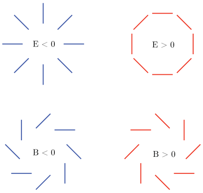
Figure 4: Examples of $E$- and $B$-mode patterns of polarization

To characterize the statistics of the CMB perturbations, only four power spectra are needed, those for $T$, $E$, $B$ and the cross correlation between $T$ and $E$. The cross correlation between $B$ and $E$ or $B$ and $T$ vanishes if there are no parity-violating interactions because $B$ has the opposite parity to $T$ or $E$. The power spectra are defined as the rotationally invariant quantities $C_{T\ell}={1\over 2\ell+1}\sum_{m}\langle a_{T,\ell m}^{*}a_{T,\ell m}\rangle$, $C_{E\ell}={1\over 2\ell+1}\sum_{m}\langle a_{E,\ell m}^{*}a_{E,\ell m}\rangle$, $C_{B\ell}={1\over 2\ell+1}\sum_{m}\langle a_{B,\ell m}^{*}a_{B,\ell m}\rangle$, and $C_{C\ell}={1\over 2\ell+1}\sum_{m}\langle a_{T,\ell m}^{*}a_{E,\ell m}\rangle$. The brackets $\langle\cdots\rangle$ denote ensemble averages.

Polarization is generated by Thomson scattering between photons and electrons, which means that polarization cannot be generated after recombination (except for re-ionization, which we shall discuss later). But Thomson scattering is not enough. The radiation incident on the electrons must also be anisotropic. In fact, its intensity needs to have a quadrupole moment. This requirement of having both Thomson scattering and anisotropies is what makes polarization relatively small. After recombination, anisotropies grow by free streaming, but there is no scattering to generate polarization. Before recombination there were so many scatterings that they erased any anisotropy present in the photon–baryon fluid.

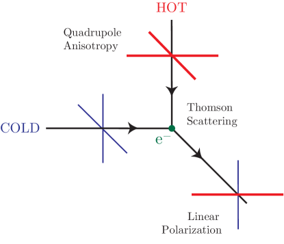
Figure 5: Thomson scattering of radiation where quadrupole anisotropy generates linear polarization

In the context of anisotropies induced by density perturbations, velocity gradients in the photon–baryon fluid are responsible for the quadrupole that generates polarization. Let us consider a scattering occurring at position $\hbox{\boldmath{$x$}}_{0}$: the scattered photons came from a distance of order the mean free path ($\lambda_{T}$) away from this point. If we are considering photons traveling in direction $\hat{n}$, they roughly come from $\hbox{\boldmath{$x$}}=\hbox{\boldmath{$x$}}_{0}+\lambda_{T}\hbox{\boldmath{$\hat{n}$}}$. The photon–baryon fluid at that point was moving at velocity $\hbox{\boldmath{$v$}}(\hbox{\boldmath{$x$}})\approx\hbox{\boldmath{$v$}}(\hbox{\boldmath{$x$}}_{0})+\lambda_{T}{\hbox{\boldmath{$\hat{n}$}}}_{i}\partial_{i}{\hbox{\boldmath{$v$}}}(\hbox{\boldmath{$x$}}_{0})$. Due to the Doppler effect the temperature seen by the scatterer at $\hbox{\boldmath{$x$}}_{0}$ is $\delta T(\hbox{\boldmath{$x$}}_{0},\hbox{\boldmath{$\hat{n}$}})=\hbox{\boldmath{$\hat{n}$}}\cdot[\hbox{\boldmath{$v$}}(\hbox{\boldmath{$x$}})-\hbox{\boldmath{$v$}}(\hbox{\boldmath{$x$}}_{0})]\approx\lambda_{T}{\hbox{\boldmath{$\hat{n}$}}}_{i}{\hbox{\boldmath{$\hat{n}$}}}_{j}\partial_{i}{\hbox{\boldmath{$v$}}}_{j}(\hbox{\boldmath{$x$}}_{0})$, which is quadratic in $\hat{n}$ (i.e., it has a quadrupole). Velocity gradients in the photon–baryon fluid lead to a quadrupole component of the intensity distribution, which, through Thomson scattering, is converted into polarization.

The polarization of the scattered radiation field, expressed in terms of the Stokes parameters $Q$ and $U$, is given by $(Q+iU)\propto\sigma_{T}\int d\Omega^{\prime}({\bf m}\cdot\hat{{\bf n}}^{\prime})^{2}T(\hat{{\bf n}}^{\prime})$ $\propto\lambda_{p}{\bf m}^{i}{\bf m}^{j}\partial_{i}v_{j}|_{\tau_{\rm LS}}$, where $\sigma_{T}$ is the Thomson scattering cross-section and we have written the scattering matrix as $P({\bf m},\hat{{\bf n}}^{\prime})=-3/4\sigma_{T}({\bf m}\cdot\hat{{\bf n}}^{\prime})^{2}$, with ${\bf m}=\hat{{\bf e}}_{1}+i\hat{{\bf e}}_{2}$ . In the last step, we integrated over all directions of the incident photons $\hat{{\bf n}}^{\prime}$. As photons decouple from the baryons, their mean free path grows very rapidly, so a more careful analysis is needed to obtain the final polarization:

$$(Q+iU)(\hat{{\bf n}})\approx\epsilon\delta\tau_{\rm LS}{\bf m}^{i}{\bf m}^{j}\partial_{i}v_{j}|_{\tau_{\rm LS}},$$ (91)

where $\delta\tau_{\rm LS}$ is the width of the last scattering surface and gives a measure of the distance that photons travel between their last two scatterings, and $\epsilon$ is a numerical constant that depends on the shape of the visibility function. The appearance of ${\bf m}^{i}{\bf m}^{j}$ in Eq. (91) ensures that $(Q+iU)$ transforms correctly under rotations of $(\hat{{\bf e}}_{1},\hat{{\bf e}}_{2})$.

If we evaluate Eq. (91) for each Fourier mode and combine them to obtain the total power, we get the equivalent of Eq. (88),

$$\ell(\ell+1)C_{E\ell}\approx A\epsilon^{2}(1+3R)^{2}(k_{*}\delta\tau_{\rm LS})^{2}\sin^{2}(k_{*}c_{s}\tau_{\rm LS}),$$ (92)

where we are assuming $n=1$ and that $\ell$ is large enough that factors like $(\ell+2)!/(\ell-2)!\approx\ell^{4}$. The extra $k_{*}$ in Eq. (92) originates in the gradient in Eq. (91). The large-angular scale polarization is greatly suppressed by the $k\delta\tau_{\rm LS}$ factor. Correlations over large angles can only be created by the long-wavelength perturbations, but these cannot produce a large polarization signal because of the tight coupling between photons and electrons prior to recombination. Multiple scatterings make the plasma very homogeneous; only wavelengths that are small enough to produce anisotropies over the mean free path of the photons will give rise to a significant quadrupole in the temperature distribution, and thus to polarization. Wavelengths much smaller than the mean free path decay due to photon diffusion (Silk damping) and so are unable to create a large quadrupole and polarization. As a result polarization peaks at the scale of the mean free path.

On sub-degree angular scales, temperature, polarization, and the cross-correlation power spectra show acoustic oscillations. In the polarization and cross-correlation spectra the peaks are much sharper. The polarization is produced by velocity gradients of the photon—baryon fluid at the last scatteringsurface. The temperature receives contributions from density and velocity perturbations, and the oscillations in each partially cancel one another, making the features in the temperature spectrum less sharp. The dominant contribution to the temperature comes from the oscillations in the density [Eq. (0.8.2)], which are out of phase with the velocity. This explains the difference in location between the temperature and polarization peaks. The extra gradient in the polarization signal, Eq. (91), explains why its overall amplitude peaks at a smaller angular scale.

Now, as photons travel in the metric perturbed by a GW [$ds^{2}=a^{2}(\tau)$ $[-d\tau^{2}$ $+(\delta_{ij}+h^{T}_{ij})dx^{i}dx^{j}]$], they get redshifted or blueshifted depending on their direction of propagation relative to the direction of propagation of the GW and the polarization of the GW. For example, for a GW travelling along the $z$ axis, the frequency shift is given by

$${1\over\nu}{d\nu\over d\tau}={1\over 2}\ \hat{n}^{i}\hat{n}^{j}{\dot{h}}^{T(\pm)}_{ij}={1\over 2}\ (1-\cos^{2}\theta)e^{\pm i2\phi}\ \ \dot{h}_{t}\ \exp(i\bf k\cdot\bf x),$$ (93)

where $(\theta,\phi)$ describe the direction of propagation of the photon, the $\pm$ correspond to the different polarizations of the GW, and $h_{t}$ gives the time-dependent amplitude of the GW. During the matter-dominated era, for example, $h_{t}=3j_{1}(k\tau)/k\tau$: time changes in the metric lead to frequency shifts (or equivalently shifts in the temperature of the black body spectrum). Notice that the angular dependence of this frequency shift is quadrupolar in nature. As a result, the temperature fluctuations induced by this effect as photons travel between successive scatterings before recombination produce a quadrupole intensity distribution, which, through Thomson scattering, lead to polarization. Both $E$ and $B$ power spectra are generated by GW. The current push to improve polarization measurements follows from the fact that density perturbations, to linear order in perturbation theory, cannot create any $B$-type polarization. As a rough rule of thumb, the amplitude of the peak in the $B$-mode power spectrum for GW is

[ℓ(ℓ+1)C_Bl/ 2π]^1/2=0.024 (V^1/4/ 10^16GeV)^2 μK

where

$$V^{1/4}\simeq 6.7\,r^{1/4}\,\times 10^{16}\,{\rm GeV}$$ (94)

is the energy scale of inflation. A future experiment like CMBPol [18] can probe values of $r$ as small as $10^{-2}$, corresponding to an inflation energy scale of about $2\times\times 10^{16}$ GeV. Furthermore, using the consistency relation $r=\epsilon$ valid in one-single field models of inflation, one deduces that

$$\frac{\Delta\phi}{m_{\rm Pl}}\simeq\left(\frac{r}{10^{-2}}\right)^{1/2},$$ (95)

meaning that a future measurement of the $B$-mode of CMB polarization will imply an inflaton excursus of Planckian values. Therefore, A future measurement of the $B$-mode polarization of the CMB will allow a determination of the value of the energy scale of inflation. This explains the utility of CMB polarization measurements as probes of the physics of inflation. A detection of primordial $B$-mode polarization would also demonstrate that inflation occurred at a very high energy scale, and that the inflaton traversed a super-Planckian distance in field space.

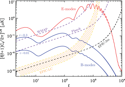
Figure 6: E- and B-mode power spectra for a tensor-to-scalar ratio saturating the current bounds, $r=0.3$ and for $r=0.01$. Shown are the experimental sensitivities of WMAP, Planck and two different realizations of CMBPol (EPIC-LC and EPIC-2m)

0.8.4 Dark matter

Another topic we marginally touched in the lectures was dark matter, while we will not discuss the dark energy puzzle we did not have time to cover in detail. This section is taken verbatim from Freese [19]. We thank K. Freese for granting permission. The evidence that 95% of the mass of galaxies and clusters is made of some unknown component of Dark Matter (DM) comes from (i) rotation curves (out to tens of kpc), (ii) gravitational lensing (out to 200 kpc), and (iii) hot gas in clusters. They lead us to believe that DM makes up about 30% of the entire energy of the universe.

In the 1970s, Ford and Rubin discovered that rotation curves of galaxies are flat. The velocities of objects (stars or gas) orbiting the centres of galaxies, rather than decreasing as a function of the distance from the galactic centres as had been expected, remain constant out to very large radii. Similar observations of flat rotation curves have now been found for all galaxies studied, including our Milky Way. The simplest explanation is that galaxies contain far more mass than can be explained by the bright stellar objects residing in galactic disks. This mass provides the force to speed up the orbits. To explain the data, galaxies must have enormous dark haloes made of unknown matter. Indeed, more than 95% of the mass of galaxies consists of dark matter. The baryonic matter which accounts for the gas and disk cannot alone explain the galactic rotation curve. However, adding a DM halo allows a good fit to data.

The limitations of rotation curves are that one can only look out as far as there is light or neutral hydrogen (21 cm), namely to distances of tens of kpc. Thus one can see the beginnings of DM haloes, but cannot trace where most of the DM is. The lensing experiments discussed in the next section go beyond these limitations.

Einstein’s theory of General Relativity predicts that mass bends, or lenses, light. This effect can be used to gravitationally ascertain the existence of mass even when it emits no light. Lensing measurements confirm the existence of enormous quantities of DM both in galaxies and in clusters of galaxies. Observations are made of distant bright objects such as galaxies or quasars. As the result of intervening matter, the light from these distant objects is bent towards the regions of large mass. Hence there may be multiple images of the distant objects, or, if these images cannot be individually resolved, the background object may appear brighter. Some of these images may be distorted or sheared. The Sloan Digital Sky Survey used weak lensing (statistical studies of lensed galaxies) to conclude that galaxies, including the Milky Way, are even larger and more massive than previously thought, and require even more DM out to great distances. Again, the predominance of DM in galaxies is observed. The key success of the lensing of DM to date is the evidence that DM is seen out to much larger distances than could be probed by rotation curves: the DM is seen in galaxies out to 200 kpc from the centres of galaxies, in agreement with N-body simulations. On even larger Mpc scales, there is evidence for DM in filaments (the cosmic web). Another piece of gravitational evidence for DM is the hot gas in clusters. The X-ray data indicates the presence of hot gas. The existence of this gas in the cluster can only be explained by a large DM component that provides the potential well to hold on to the gas. In summary, the evidence is overwhelming for the existence of an unknown component of DM that comprises 95% of the mass in galaxies and clusters.

There is another basic reason why DM is necessary: to form structures as we observe them. Let us assume that the matter content of the universe is dominated by a pressureless and self-gravitating fluid. This approximation holds if we are dealing with the evolution of the perturbations in the DM component or in case we are dealing with structures whose size is much larger than the typical Jeans scale length of baryons. Let us also define $\rm{\bf x}$ to be the co-moving coordinate and ${\bf r}=a(t){\bf x}$ the proper coordinate, $a(t)$ being the cosmic expansion factor. Furthermore, if ${\bf v}=\dot{\bf r}$ is the physical velocity, then ${\bf v}=\dot{a}{\bf x}+{\bf u}$, where the first term describes the Hubble flow, while the second term, ${\bf u}=a(t)\dot{\bf x}$, gives the peculiar velocity of a fluid element which moves in an expanding background.

In this case the equations that regulate the Newtonian description of the evolution of density perturbations are the continuity equation:

$${\partial\delta\over\partial t}+\nabla\cdot[(1+\delta){\bf u}]=0\,,$$ (96)

which gives the mass conservation, the Euler equation

$${\partial{\bf u}\over\partial t}+2H(t){\bf u}+({\bf u}\cdot\nabla){\bf u}=-{\nabla\phi\over a^{2}}\,,$$ (97)

which gives the relation between the acceleration of the fluid element and the gravitational force, and the Poisson equation

$$\nabla^{2}\phi=4\pi G\bar{\rho}a^{2}\delta$$ (98)

which specifies the Newtonian nature of the gravitational force. In the above equations, $\nabla$ is the gradient computed with respect to the co-moving coordinate ${\bf x}$, $\phi({\bf x})$ describes the fluctuations of the gravitational potential, and $H(t)=\dot{a}/a$ is the Hubble parameter at the time $t$. Its time-dependence is given by $H(t)=E(t)H_{0}$, where

$$E(z)=[(1+z)^{3}\Omega_{m}+(1+z)^{2}(1-\Omega_{m}-\Omega_{DE})+(1+z)^{3(1+w)}\Omega_{DE}]^{1/2}.$$ (99)

In the case of small perturbations, these equations can be linearized by neglecting all the terms which are of second order in the fields $\delta$ and ${\bf u}$. In this case, using the Euler equation to eliminate the term $\partial\rm{\bf u}/\partial t$, and using the Poisson equation to eliminate $\nabla^{2}\phi$, one ends up with

$${\partial^{2}\delta\over\partial t^{2}}+2H(t){\partial\delta\over\partial t}-4\pi G\bar{\rho}\delta=0\,.$$ (100)

This equation describes the Jeans instability of a pressureless fluid, with the additional “Hubble drag” term $2H(t){\partial\delta/\partial t}$, which describes the counter-action of the expanding background on the perturbation growth. Its effect is to prevent the exponential growth of the gravitational instability taking place in a non-expanding background. The solution of the above equation can be cast in the form:

$$\delta({\bf x},t)=\delta_{+}({\bf x},t_{i})D_{+}(t)+\delta_{-}({\bf x},t_{i})D_{-}(t)\,,$$ (101)

where $D_{+}$ and $D_{-}$ describe the growing and decaying modes of the density perturbation, respectively. In the case of an Einstein–de-Sitter (EdS) universe ($\Omega_{m}=1$, $\Omega_{DE}=0$), it is $H(t)=2/(3t)$, so that $D_{+}(t)=(t/t_{i})^{2/3}$ and $D_{-}(t)=(t/t_{i})^{-1}$. The fact that $D_{+}(t)\propto a(t)$ for an EdS universe should not be surprising. Indeed, the dynamical time-scale for the collapse of a perturbation of uniform density $\rho$ is $t_{\rm dyn}\propto(G\rho)^{-1//2}$, while the expansion time-scale for the EdS model is $t_{\rm exp}\propto(G\bar{\rho})^{-1//2}$, where $\bar{\rho}$ is the mean cosmic density. Since for a linear (small) perturbation it is $\rho\simeq\bar{\rho}$, then $t_{\rm dyn}\sim t_{\rm exp}$, thus showing that the cosmic expansion and the perturbation evolution take place at the same pace. This argument also leads to understanding the behaviour for a $\Omega_{m}<1$ model. In this case, the expansion time scale becomes shorter than the above one at the redshift at which the universe recognizes that $\Omega_{m}<1$. This happens at $1+z\simeq\Omega_{m}^{-1/3}$ or at $1+z\simeq\Omega_{m}^{-1}$ in the presence or absence of a cosmological constant term, respectively. Therefore, after this redshift, cosmic expansion takes place at a quicker pace than gravitational instability, with the result that the perturbation growth is frozen.

The exact expression for the growing model of perturbations is given by

$$D_{+}(z)\,=\,{5\over 2}\,\Omega_{m}E(z)\,\int_{z}^{\infty}{1+z^{\prime}\over E(z^{\prime})^{3}}\,dz^{\prime}.$$ (102)

The EdS has the faster evolution, while the slowing down of the perturbation growth is more apparent for the open low-density model, the presence of a cosmological constant providing an intermediate degree of evolution. The key point is, however, that a pressureless fluid such as DM is needed for the perturbations to grow to give rise to collapsed objects. Baryon perturbations, being coupled to photons till the last-scattering epoch, feel a non-vanishing pressure and therefore they may not grow. After the last-scattering stage, the baryons fall into the gravitational potential generated by DM and the baryonic perturbations may promptly catch up with those of DM.

Dark matter candidates

There is a plethora of dark matter candidates. MACHOs, or Massive Compact Halo Objects, are made of ordinary matter in the form of faint stars or stellar remnants; they could also be primordial black holes or mirror matter. However, there are not enough of them to completely resolve the question. Of the non-baryonic candidates, the most popular are the WIMPS (Weakly Interacting Massive Particles) and the axions, as these particles have been proposed for other reasons in particle physics. Ordinary massive neutrinos are too light to be cosmologically significant, though sterile neutrinos remain a possibility. Other candidates include primordial black holes, non-thermal WIMPzillas, and Kaluza–Klein particles which arise in higher dimensional theories.

About axions, the good news is that cosmologists do not need to “invent” new particles. Two candidates already exist in particle physics for other reasons: axions and WIMPs. Axions with masses in the range $10^{-(3-6)}$ eV arise in the Peccei–Quinn solution to the strong-CP problem in the theory of strong interactions.

WIMPs are also natural dark matter candidates from particle physics. These particles, if present in thermal abundances in the early universe, annihilate with one another so that a predictable number of them remain today. The relic density of these particles comes out to be the right value:

$$\Omega_{\rm DM}h^{2}=(3\times 10^{-26}{\rm cm}^{3}/{\rm s})/\langle\sigma v\rangle_{\rm A}$$ (103)

where the annihilation cross-section $\langle\sigma v\rangle_{\rm A}$ of weak interaction strength automatically gives the right answer. The reason why the final abundance is inversely proportional to the annihilation cross-section is rather clear: the larger the annihilation cross-section, the more WIMPs annihilate and the fewer of them are left behind. Furthermore, annihilation is not eternal: owing to the expansion of the universe, annihilation stops when its rate becomes smaller than the expansion rate of the universe. When this happens, the abundance is said to freeze-out.

Figure 7: The abundance of WIMPs of a given mass $m$ as a function of temperature and for various annihilation cross-sections

This coincidence is known as ‘the WIMP miracle’ and is the reason why WIMPs are taken so seriously as DM candidates. The best WIMP candidate is motivated by Supersymmetry (SUSY): the lightest neutralino in the Minimal Supersymmetric Standard Model. Supersymmetry in particle theory is designed to keep particle masses at the right value. As a consequence, each particle we know has a partner: the photino is the partner of the photon, the squark is the quark’s partner, and the selectron is the partner of the electron. The lightest superysmmetric partner is a good dark matter candidate.

There are several ways to search for dark WIMPs. SUSY particles may be discovered at the LHC as missing energy in an event. In that case one knows that the particles live long enough to escape the detector, but it will still be unclear whether they are long-lived enough to be the dark matter. Thus complementary astrophysical experiments are needed. In direct detection experiments, the WIMP scatters off a nucleus in the detector, and a number of experimental signatures of the interaction can be detected. In indirect detection experiments, neutrinos that arise as annihilation products of captured WIMPs exit from the Sun and can be detected on Earth. Another way to detect WIMPs is to look for anomalous cosmic rays from the Galactic Halo: WIMPs in the Halo can annihilate with one another to give rise to antiprotons, positrons, or neutrinos. In addition, neutrinos, gamma rays, and radio waves may be detected as WIMP annihilation products from the Galactic Centre. For lack of time these issues were not discussed extensively in the lectures. The interested reader may find more about these issues in Ref. [20].

0.9 Conclusions

The period when we say that cosmology is entering a golden age has already passed: cosmology is in the middle of its golden age. Present observational data pose various puzzles whose solutions might either be around the corner or decades far in the future. It will require some young and creative researcher sitting in this room to solve them. This is why the cosmological puzzles are dark, but the future is brighter.

References

- [1] A. D. Linde, Particle Physics and Inflationary Cosmology (Harwood, Chur, Switzerland, 1990) and references therein.
- [2] E. W. Kolb and M. S. Turner, The Early Universe (Addison-Wesley, Redwood City, CA, 1990).
- [3] See http://cds.cern.ch/record/316856/files/9612138.pdf.
- [4] Michael Turner’s lectures, p353, of Quantitative Particle Physics: Cargese 1992.
- [5] . A. Linde in Physical cosmology : 25th anniversary of the cosmic background radiation discovery, Gif-sur-Yvette : Ed. Frontieres, 1991.
- [6] A. R. Liddle and D. H. Lyth, Phys. Rep. 231, 1 (1993) and references therein.
- [7] A. R. Liddle and D. H. Lyth, Cosmological Inflation and Large-Scale Structure (Cambridge University Press, 2000) and references therein.
- [8] D. H. Lyth and A. Riotto, Phys. Rep. 314, 1 (1999) and references therein.
- [9] A. Riotto, arXiv:hep-ph/0210162 and references therein.
- [10] For a review, see N. Bartolo, S. Matarrese, and A. Riotto, arXiv:astro-ph/0703496 and references therein.
- [11] E. J. Copeland, M. Sami, and S. Tsujikawa, Int. J. Mod. Phys. D 15, 1753 (2006) and references therein.
- [12] E. Komatsu et al. [WMAP Collaboration], Astrophys. J. Suppl. 180, 330 (2009) [arXiv:0803.0547 [astro-ph]].
- [13] For a review, see, for instance, N. A. Bahcall, J. P. Ostriker, S. Perlmutter, and P. J. Steinhardt, Science 284, 1481 (1999).
- [14] R. K. Sachs and A. M. Wolfe, Astrophys. J. 147, 73 (1967).
- [15] S. Dodelson, Modern Cosmology (Academic Press, New York, 2003).
- [16] V. F. Mukhanov, H. A. Feldman, and R. H. Brandenberger, Phys. Rep. 215, 203 (1992) and references therein.
- [17] M. Zaldarriaga, astro-ph/0305272.
- [18] S. Dodelson et al., CMBPol Science White Paper submitted to the US Astro2010 Decadal Survey, arXiv:0902.3796v1.
- [19] K. Freese, EAS Publ. Ser. 36, 113 (2009) doi:10.1051/eas/0936016 [arXiv:0812.4005 [astro-ph]].
- [20] G. Bertone, D. Hooper, and J. Silk, Phys. Rep. 405, 279 (2005).