A unique signal of excited bosons in dijet data from $\bm{pp}\,$-collisions

Abstract

With this note we would like to draw attention to a possible novel signal of new physics in dijet data at the hadron colliders. Usually it is accepted that all exotic models predict that these two jets populate the central (pseudo)rapidity region where $y_{1,2}\simeq 0$. Contrary, the excited bosons do not contribute into this region, but produce an excess of dijet events over the almost flat QCD background in $\chi=\exp|y_{1}-y_{2}|$ away from this region.

I Introduction

Due to the largest cross section of all processes at the hadron colliders dijet production opens a possibility to search for a signal of new physics in the very early data. In particular, a bump in the dijet invariant mass spectrum would indicate the presence of a resonance decaying into two energetic partons. However, due to the huge QCD background the bump could be just a statistical fluctuation of the limited integrated luminosity of the fist data. Besides this, the bump in the invariant mass distribution stems from the Breit–Wigner propagator form, which is characteristic for any type of the resonance regardless of its other properties, like spin, internal quantum number, etc. Therefore, other observables are necessary in order to confirm the bump and to reveal the resonance properties.

The distribution of dijets over the polar angle $\theta$  is directly sensitive to the resonance spin and the dynamics of the underlying process. While the QCD processes are dominated by $t$-channel gluon exchanges, which lead to a Rutherford-like distribution $1/(1-\cos\theta)^{2}$, exotic physics processes proceed mainly through the $s$-channel, where the spin of the resonance uniquely defines the angular distribution. For high-mass resonances and practically massless partons it is convenient to use the helicity formalism, since the helicity is a good quantum number for massless particles.

For example, the decay angular distribution in the centre-of-momentum frame of a particle with spin-$s$ and helicity $\lambda$ with $-s\leq\lambda\leq s$ decaying into two massless particles with helicities $\lambda_{1}$ and $\lambda_{2}$ can be written as Haber

$$\frac{{\rm d}\Gamma_{s}}{{\rm d}\cos\theta\;{\rm d}\phi}=\frac{1}{64\pi^{2}M}\,|\,{\cal M}^{s\lambda}_{\lambda_{1}\lambda_{2}}(\theta,\phi)|^{2},$$ (1)

where the helicity amplitude

$${\cal M}^{s\lambda}_{\lambda_{1}\lambda_{2}}(\theta,\phi)=\sqrt{\frac{2s+1}{4\pi}}\,e^{i(\lambda-\delta)\phi}\,d^{s}_{\lambda\delta}(\theta)\,{\cal M}^{s}_{\lambda_{1}\lambda_{2}}\vspace{0.2cm}$$ (2)

is expressed through the difference $\delta\equiv\lambda_{1}-\lambda_{2}$ with $-s\leq\delta\leq s$ and the reduced decay amplitude ${\cal M}^{s}_{\lambda_{1}\lambda_{2}}$, which is a function of $s$ and the helicities of the outgoing particles, but is independent on the azimuthal ($\phi$) and the polar ($\theta$) angles. The $\theta$-dependence is concentrated only in the well-known $d$-functions $d^{s}_{\lambda\delta}(\theta)$.

The absolute value of the dijet rapidity difference is related to the polar scattering angle $\theta$ with respect to the beam axis by $\Delta y\equiv|y_{1}-y_{2}|=\ln[(1+|\cos\theta|)/(1-|\cos\theta|)]\geq 0$ and is invariant under boosts along the beam direction. The choice of the other variable $\chi\equiv\exp(\Delta y)=(1+|\cos\theta|)/(1-|\cos\theta|)\geq 1$ is motivated by the fact that Rutherford scattering does not depend on it.

In the next section we will analyse a model independent signal of new physics using distributions on these variables and their combinations.

II A unique signal of excited bosons

Let us consider different possibilities for the spin of a resonance and its possible interactions with partons. The simplest case of the resonance production of a (pseudo)scalar particle $h$ with spin 0 in $s$-channel leads to a uniform decay distribution on the scattering angle

$$\frac{{\rm d}\Gamma_{0}(h\to q\bar{q})}{{\rm d}\cos\theta}\propto|d^{\,0}_{00}|\,^{2}\sim 1.$$ (3)

The spin-1/2 fermion resonance, like an excited quark $q^{*}$, leads to asymmetric decay distributions for the given spin parton configurations

$$\frac{{\rm d}\Gamma_{1/2}(q^{*}\to qg)}{{\rm d}\cos\theta}\propto|d^{1/2}_{1/2,1/2}|\,^{2}\sim 1+\cos\theta$$ (4)

and

$$\frac{{\rm d}\Gamma_{1/2}(q^{*}\to qg)}{{\rm d}\cos\theta}\propto|d^{1/2}_{1/2,-1/2}|\,^{2}\sim 1-\cos\theta.$$ (5)

However, the choice of the variables, which depend on the absolute value of $\cos\theta$, cancels out the apparent dependence on $\cos\theta$. In other words, the distributions (4) and (5) for dijet events look like uniform distributions on $\Delta y$ and $\chi$.

According to the simple formula

$$\frac{{\rm d}\Gamma}{{\rm d}(\Delta y/\chi)}=\frac{{\rm d}\cos\theta}{{\rm d}(\Delta y/\chi)}\;\frac{{\rm d}\Gamma}{{\rm d}\cos\theta}\,,$$ (6)

the uniform distribution leads to kinematical peaks at small values of $\Delta y=0$ (the dotted curve in the left panel of Fig. 1)

$$\frac{{\rm d}\Gamma_{0}}{{\rm d}\Delta y}\propto\frac{{\rm e}^{\Delta y}}{({\rm e}^{\Delta y}+1)^{2}}$$ (7)

and $\chi=1$ (the dotted curve in the right panel of Fig. 1)

$$\frac{{\rm d}\Gamma_{0}}{{\rm d}\chi}\propto\frac{1}{(\chi+1)^{2}}.$$ (8)

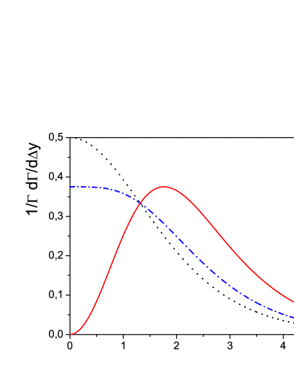
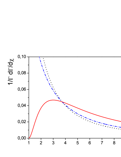
Figure 1: The normalized angular dijet distributions as functions of the absolute value of the rapidity difference (left) and the $\chi$ variable (right) for the scalar (or/and spin-1/2), the gauge bosons with the minimal coupling and the excited bosons are shown correspondingly with the dotted, dash-dotted and solid curves.

A novel situation can occur for the spin-1 resonances, which appear as new gauge bosons in the extended gauge symmetry groups. We will consider all possible interactions of such bosons with the ordinary fermions. There are two different possibilities.

The gauge bosons, which are associated with additional $U(1)^{\prime}$ gauge symmetry (or transform under the adjoint representation of the extra gauge group), are generally called $Z^{\prime}(\bm{W}^{\prime})$ particles. They have minimal gauge interactions with the known light fermions

$${\cal L}_{Z^{\prime}}=\sum_{f}\left(g^{f}_{LL}\;\overline{\psi^{f}_{L}}\gamma^{\mu}\psi^{f}_{L}+g^{f}_{RR}\;\overline{\psi^{f}_{R}}\gamma^{\mu}\psi^{f}_{R}\right)Z^{\prime}_{\mu}\,,$$ (9)

which preserve the fermion chiralities and possess maximal helicities $\lambda=\pm 1$. At a symmetric $pp$ collider, like the LHC, such interactions lead to the specific symmetric angular distribution of the resonance decay products over the polar angle $\theta$,

$$\frac{{\rm d}\Gamma_{1}(Z^{\prime}\to q\bar{q})}{{\rm d}\cos\theta}\propto|d^{1}_{11}|^{2}+|d^{1}_{-11}|^{2}\sim 1+\cos^{2}\theta\,.$$ (10)

Similar to the uniform distribution, eq. (10) leads to kinematical peaks also at small values of $\Delta y=0$ (the dash-dotted curve in the left panel of Fig. 1)

$$\frac{{\rm d}\Gamma^{\prime}_{1}}{{\rm d}\Delta y}\propto\frac{{\rm e}^{\Delta y}({\rm e}^{2\Delta y}+1)}{({\rm e}^{\Delta y}+1)^{4}}$$ (11)

and $\chi=1$ (the dash-dotted curve in the right panel of Fig. 1)

$$\frac{{\rm d}\Gamma^{\prime}_{1}}{{\rm d}\chi}\propto\frac{\chi^{2}+1}{(\chi+1)^{4}}.$$ (12)

Another possibility is the resonance production and decay of new longitudinal spin-1 bosons with helicity $\lambda=0$. The new gauge bosons with such properties arise in many extensions Gia of the Standard Model (SM), which solve the Hierarchy Problem. They transform as doublets $(Z^{*}\;W^{*})$ under the fundamental representation of the SM $SU(2)_{W}$ group like the SM Higgs boson.

While the $Z^{\prime}$ bosons with helicities $\lambda=\pm 1$ are produced in left(right)-handed quark and right(left)-handed antiquark fusion, the longitudinal $Z^{*}$ bosons can be produced through the anomalous chiral couplings with the ordinary light fermions

$${\cal L}_{Z^{*}}=\sum_{f}\left(\frac{g^{f}_{LR}}{M}\,\overline{\psi^{f}_{L}}\sigma^{\mu\nu}\psi^{f}_{R}\;\partial_{[\mu}\bar{Z}^{*}_{\nu]}+\frac{g^{f}_{RL}}{M}\,\overline{\psi^{f}_{R}}\sigma^{\mu\nu}\psi^{f}_{L}\;\partial_{[\mu}Z^{*}_{\nu]}\right)$$ (13)

in left-handed or right-handed quark-antiquark fusion proposal . The anomalous interactions (13) are generated on the level of the quantum loop corrections and can be considered as effective interactions. The gauge doublets, coupled to the tensor quark currents, are some types of “excited” states as far as the only orbital angular momentum with $L=1$ contributes to the total angular moment, while the total spin of the system is zero. This property manifests itself in their derivative couplings to fermions and a different chiral structure of the interactions in contrast to the minimal gauge interactions (9).

The anomalous couplings lead to a different angular distribution of the resonance decay

$$\frac{{\rm d}\Gamma^{*}_{1}(Z^{*}\to q\bar{q})}{{\rm d}\cos\theta}\propto|d^{1}_{00}|\,^{2}\sim\cos^{2}\theta.$$ (14)

than the previously considered ones. At first sight, the small difference between the distributions (10) and (14) seems unimportant. However, the absence of the constant term in the latter case results in novel experimental signatures.

First of all, the uniform distribution (3) for scalar and spin-1/2 particles and the distribution (10) for gauge vector bosons with minimal coupling include a nonzero constant term, which leads, to a kinematic singularity in the transverse momentum distribution of the final parton

$$\frac{{\rm d}\cos\theta}{{\rm d}p_{\rm T}}\sim\frac{1}{\cos\theta}\propto\frac{1}{\sqrt{(M/2)^{2}-p^{2}_{\rm T}}}$$ (15)

in the narrow width approximation $\Gamma\ll M$

$$\frac{1}{(s-M^{2})^{2}+M^{2}\Gamma^{2}}\approx\frac{\pi}{M\Gamma}\,\delta(s-M^{2}).$$ (16)

After smearing from the resonance finite width the singularity is transformed into the well-known Jacobian peak (the dash-dotted curve in the left panel of Fig. 2). The analytic expression of the $p_{\rm T}$ distribution can be found in Barger .

Using the same method one can derive the analogous distribution for the excited bosons (the solid curve in the left panel of Fig. 2).

$$\frac{{\rm d}\Gamma^{*}_{1}}{{\rm d}p_{\rm T}}\propto\frac{p_{\rm T}}{\sqrt{\sqrt{\left(4p^{2}_{\rm T}-M^{2}\right)^{2}+\Gamma^{2}M^{2}}+4p^{2}_{\rm T}-M^{2}}}.$$ (17)

In contrast to the previous case, the pole in the decay distribution of the excited bosons is canceled out and the final parton $p_{\rm T}$ distribution has a broad smooth hump ICTP with a maximum at $p_{\rm T}=\sqrt{(M^{2}+\Gamma^{2})/8}\simeq M/\sqrt{8}$ below the kinematical endpoint $p_{\rm T}=M/2$, instead of a sharp Jacobian peak, that obscures their experimental identification as resonances. Therefore, the transverse jet momentum is not the appropriate variable for the excited boson search.

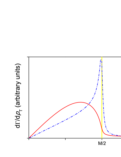
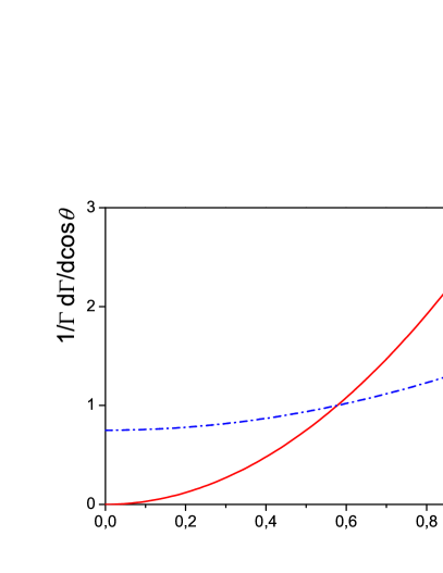
Figure 2: The final parton transverse momentum (left) and angular (right) distributions from the gauge (dash-dotted curves) and the excited (solid curves) bosons decays.

Another striking feature of the distribution (14) is the forbidden decay direction perpendicular to the boost of the excited boson in the rest frame of the latter (the Collins–Soper frame CS ). It leads to a profound dip at $\cos\theta=0$ in the Collins–Soper frame proposal in comparison with the gauge boson distribution (the right panel in Fig. 2). The same dips present also at small values of $\Delta y=0$ LaTuile10 (the solid curve in the left panel of Fig. 1)

$$\frac{{\rm d}\Gamma^{*}_{1}}{{\rm d}\Delta y}\propto\frac{{\rm e}^{\Delta y}({\rm e}^{\Delta y}-1)^{2}}{({\rm e}^{\Delta y}+1)^{4}}$$ (18)

and $\chi=1$ (the solid curve in the right panel of Fig. 1)

$$\frac{{\rm d}\Gamma^{*}_{1}}{{\rm d}\chi}\propto\frac{(\chi-1)^{2}}{(\chi+1)^{4}}.$$ (19)

It can be seen from Fig. 1 that the excited bosons have unique signature in the angular distributions. They manifest themselves through the absolute minima at small values of $\Delta y=0$ and $\chi=1$ and absolute maxima right away from the origin. So, the rapidity difference distribution reaches the absolute maximum at $\Delta y=\ln(3+\sqrt{8})\approx 1.76$ and at $\chi=3$ for the angular distribution on the dijet variable $\chi$.

III First look at preliminary LHC data

In order to satisfy to bin purity and stability for physics studies it is convenient to use equidistant binning in $\log\chi$ PLB , which corresponds to periodic cell granularity of calorimeter in $\eta$. In this case the smooth $\chi$-spectra (see eqs. (12) and (19)) transform into histograms with maximum in the lowest bin for the gauge bosons with the minimal coupling and with maximum in the bin containing value of $\chi=3+\sqrt{8}\approx 5.8$ for the excited bosons (Fig. 3).

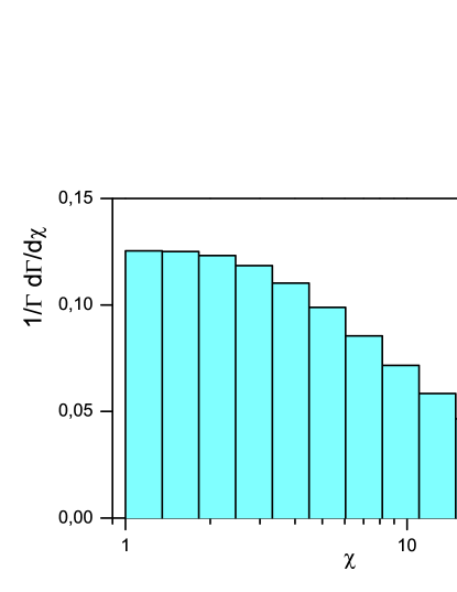
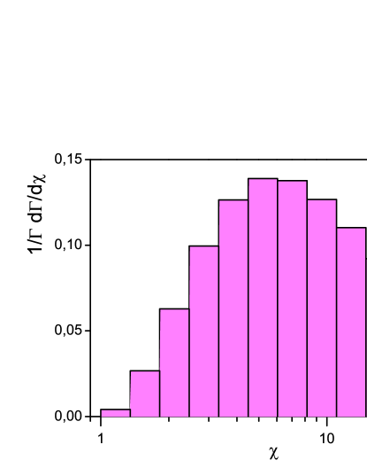
Figure 3: The normalized histograms of $\chi$-spectra for the gauge bosons with the minimal coupling (left) and for the excited bosons (right).

It is interesting to note that a shape similar to the excited-boson one (right panel in Fig. 3) can be observed in the preliminary ATLAS data PLB in $\chi$-distribution for the highest dijet mass region $M_{jj}>1200$ GeV.

Using distributions in (pseudo)rapidity and $\chi$ we can construct two useful ratios: the wide-angle to small-angle ratio

$$R_{\chi}(a,b)=\frac{N(1<\chi<a)}{N(a<\chi<b)}$$ (20)

and the centrality or $\eta$-ratio of both jets

$$R_{\eta}(a,b)=\frac{N(|\eta_{1,2}|<a)}{N(a<|\eta_{1,2}|<b)},$$ (21)

which are less affected by the systematic errors and, therefore, used for search of new physics in dijet data.

Let us suppose that we have found some bump in the dijet invariant mass distribution. For example, an excess at 550 GeV can be seen in the preliminary ATLAS data bumpATLAS for dijet processes at 0.315 nb^-1 of integrated luminosity. Then we can compare the angular distributions for “on peak” and “off peak” events, using, for example, the aforementioned ratios. Since the QCD backgrounds is dominated by the Rutherford-like distribution, we can consider, as an approximation, a simple case when the QCD dijet $\chi$-distribution is flat. It means that for the selected equal regions $b-a=a-1$ ($b=2a-1$), the $R_{\chi}$ ratio for the “off peak” events should be approximately one and does not depend on the dijet mass.

In the case, when the “on peak” events have originated from the new physics and have angular distribution different from the QCD one, this $R_{\chi}$ ratio should deviate from one. All known exotic models, besides the excited bosons, predict $R_{\chi}>1$ due to an excess at low $\chi$ values independent on $a$. In order to emphasize the effect of new physics in the case of the specific signature of the excited bosons, when $R_{\chi}<1$, we need to choose $a$ value, which minimizes the ratio

$$R_{\chi}(a,2a-1)=\frac{N_{\rm QCD}+N_{\rm new}({\rm low-}\chi)}{N_{\rm QCD}+N_{\rm new}({\rm high-}\chi)}\approx 1+\frac{N_{\rm new}({\rm low-}\chi)-N_{\rm new}({\rm high-}\chi)}{N_{\rm QCD}}<1.$$ (22)

Since $N_{\rm QCD}\propto(a-1)$, $N_{\rm new}({\rm low-}\chi)\propto(a-1)^{3}/(a+1)^{3}$ and $N_{\rm new}({\rm high-}\chi)\propto(a-1)^{3}/a^{3}-N_{\rm new}({\rm low-}\chi)$, it is possible for the choice of the parameters $a\approx 1.87$ and $b\approx 2.74$ due to the monotonic increase of the distribution for the excited bosons until the maximum at $\chi=3$. The larger value of $a\geq 1/(\sqrt[3]{2}-1)\approx 3.85$ will lead to a compensation of the contributions from low and high $\chi$-parts and $R_{\chi}\geq 1$.

For the fixed parameters $a$ and $b$ the centrality ratio $R_{\eta}$ for the QCD processes is also almost constant and should not depend on the dijet invariant mass. In the case of a presence of new physics signal this ratio could deviate from its constant value. For almost all exotic models the signal events are concentrated in the central region and usually this lead to a bump in $R_{\eta}$ distribution versus the dijet masses. By contrast to this, the signal from the excited bosons can lead to a novel signature: a dip in the distribution at the resonance mass.

We have used the CompHEP package CompHEP and the extended model with the excited bosons EMS to generate two dimensional pseudorapidity distributions for “$\,2\to 2\,$” processes proceeding through the gauge $W^{\prime}$ and excited $W^{*}$ boson resonances with the same mass 550 GeV at $\sqrt{s}=7$ TeV $pp$ collider (Fig. 4).

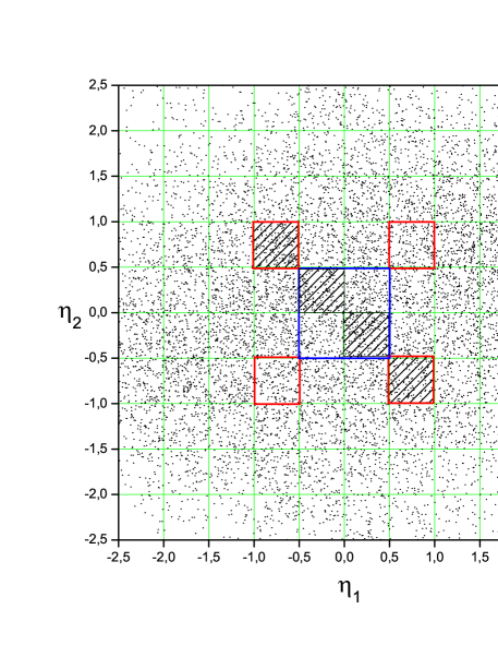
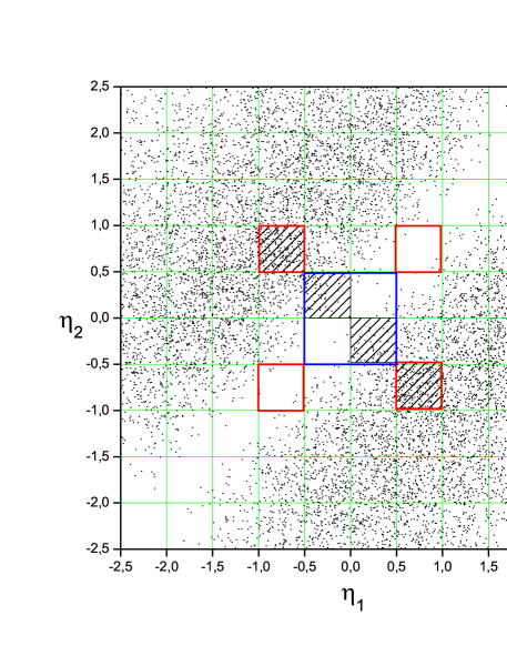
Figure 4: The two dimensional pseudorapidity distributions (scatter plots) of dijet events for the gauge bosons with the minimal coupling (left) and for the excited bosons (right). The central region $|\eta_{1,2}|<0.5$ and outer regions $0.5<|\eta_{1,2}|<1.0$ are depicted. The hatched squared regions correspond to selected events with opposite pseudorapidity signs.

The CTEQ6L parton distribution functions were used. For both final jets we impose cuts on the pseudorapidity $|\eta|<2.5$ and the transverse momentum $p_{\rm T}>30$ GeV.

To minimize the potential differences in jet response between the inner and outer dijet events one can choose the central region of the calorimeter $|\eta|<1$. Using the scatter plots in Fig. 4 one can estimate the centrality ratios (21) for the gauge

$$R^{\prime}_{\eta}(0.5,1.0)\simeq 1.08$$ (23)

and the excited

$$R^{*}_{\eta}(0.5,1.0)\simeq 0.29$$ (24)

bosons. There is dramatic difference between these two cases, which should lead to corresponding experimental signature. Since the QCD ratio $R^{\rm QCD}_{\eta}(0.5,1.0)\simeq 0.6$ is between the numbers in (23) and (24) the gauge bosons with the minimal coupling will lead to increasing the QCD ratio at the resonance mass, while the excited bosons should decrease the ratio. Just the second type of the novel signature can be observed in the distribution of the $\eta$-ratio versus the dijet invariant mass in the ATLAS data ICHEP10ATLAS in approximately the same mass range, $450~{}{\rm GeV}<M_{jj}<600$ GeV, as for the resonance bump in the dijet events bumpATLAS .

Let us stress here that the extensions of the signal region up to $|\eta|<1.3$ and the central region up to $|\eta|<0.7$ do not change drastically the QCD ratio $R^{\rm QCD}_{\eta}(0.7,1.3)\simeq 0.55$, but dilute the signal from the excited bosons, since $R^{*}_{\eta}(0.7,1.3)\simeq 0.68$.

In order to increase the sensitivity to new physics one can consider the centrality ratio only for the dijet events with opposite pseudorapidities $\left.R_{\eta}\right|_{(\eta_{1}\cdot\eta_{2})\leq 0}={\cal R}_{\eta}$ (the hatched regions in Fig. 4). In this case we get a bit larger deviation form one:

$${\cal R}^{\prime}_{\eta}(0.5,1.0)\simeq 1.12$$ (25)

for the gauge and

$${\cal R}^{*}_{\eta}(0.5,1.0)\simeq 0.25$$ (26)

for the excited bosons. But in this case we lose half of the statistics. Therefore, it is convenient to consider the distribution on $\Delta\eta\equiv|\eta_{1}-\eta_{2}|\geq 0$ for the events in the rectangle region $\Delta\eta<b$ and $\eta_{B}\equiv|\eta_{1}+\eta_{2}|<c$. The corresponding centrality ratio $R_{\Delta\eta}$ is defined as

$$R_{\Delta\eta}(a,b,c)=\left.\frac{N(\Delta\eta<a)}{N(a<\Delta\eta<b)}\right|_{\eta_{B}<c}.$$ (27)

The normalized histograms of $\Delta\eta$-spectra and the theoretical curves are shown in Fig. 5 for the following parameters values: $b=3.5$ and $c=1.5$.

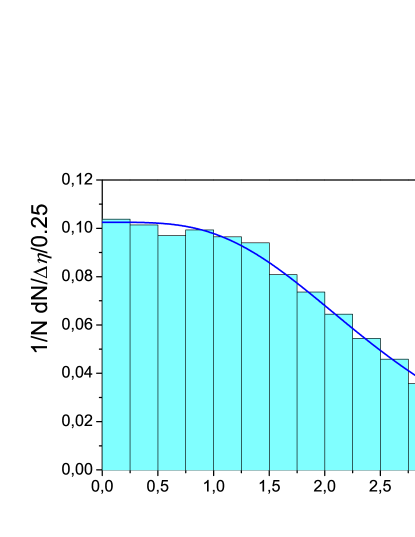
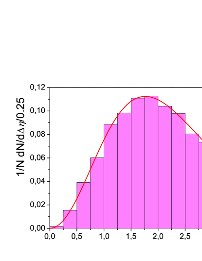
Figure 5: The normalized histograms of $\Delta\eta\,$-spectra for the gauge bosons with the minimal coupling (left) and for the excited bosons (right). The solid curves correspond to the theoretical formulae (11) and (18).

It can be seen from the figure, that the theoretical distributions describe very well the above-mentioned simulation data. In the same way as it was done for the $\chi$-distribution of the excited bosons one can maximize the deviation from the QCD ratio $R^{\rm QCD}_{\Delta\eta}=N_{\rm QCD}^{(a)}/N_{\rm QCD}^{(b-a)}$

$$R_{\Delta\eta}(a,b,c)=\frac{N_{\rm QCD}^{(a)}+N_{\rm new}^{(a)}}{N_{\rm QCD}^{(b-a)}+N_{\rm new}^{(b-a)}}\approx R^{\rm QCD}_{\Delta\eta}\left(1+\frac{N_{\rm new}^{(a)}}{N_{\rm QCD}^{(a)}}-\frac{N_{\rm new}^{(b-a)}}{N_{\rm QCD}^{(b-a)}}\right)<1.$$ (28)

Since $N_{\rm QCD}^{(a)}\propto{\rm e}^{a}-1$, $N_{\rm new}^{(a)}\propto({\rm e}^{a}-1)^{3}/({\rm e}^{a}+1)^{3}$ and $N_{\rm QCD}^{(b-a)}\propto{\rm e}^{b}-{\rm e}^{a}$, $N_{\rm new}^{(b-a)}\propto({\rm e}^{b}-1)^{3}/({\rm e}^{b}+1)^{3}-N_{\rm new}^{(a)}$, for the central calorimeter $b=1$ the minimum appears at $a=0.67$ .

IV Conclusions

In this paper we have considered the novel experimental signatures of the chiral excited bosons in the dijet data. They possess drastically different angular distributions from all previously discussed exotic models. For the special choice of parameters the wide-angle to small-angle ratio and the centrality ratio could be less than their QCD values, that will be definitely pointing out to the presence of excited bosons.

References

- (1) J.C. Collins and D.E. Soper, Phys. Rev. D 16 (1977) 2219.
- (2) H.E. Haber, “Spin formalism and applications to new physics searches”, hep-ph/9405376.
- (3) M.V. Chizhov and Gia Dvali, “Origin and Phenomenology of Weak-Doublet Spin-1 Bosons”, arXiv:0908.0924 [hep-ph].
- (4) V. Barger, A.D. Martin and R.J.N. Phillips, Z. Phys. C 21 (1983) 99.
- (5) M.V. Chizhov, “Production of new chiral bosons at Tevatron and LHC”, hep-ph/0609141.
- (6) M.V. Chizhov, V.A. Bednyakov and J.A. Budagov, Phys. Atom. Nucl. 71 (2008) 2096, arXiv:0801.4235 [hep-ph].
- (7) M.V. Chizhov, V.A. Bednyakov and J.A. Budagov, “Anomalously interacting extra neutral bosons”, arXiv:1005.2728 [hep-ph] (to be published in Nuovo Cimento B).
- (8) The ATLAS Collaboration, “Search for Quark Contact Interactions in Dijet Angular Distributions in Collisions at TeV Measured with the ATLAS Detector”, arXiv:1009.5069 [hep-ex].
- (9) G. Aad et al. (ATLAS Collaboration) “Search for New Particles in Two-Jet Final States in 7 TeV Proton-Proton Collisions with the ATLAS Detector at the LHC”, Phys. Rev. Lett. 105 (2010) 161801, arXiv:1008.2461 [hep-ex].
- (10) The ATLAS Collaboration, “Update of the search for new particles decaying into dijets in proton-proton collisions at TeV with the ATLAS detector”, ATL-CONF-2010-088.
- (11) E. Boos et al. (CompHEP Coll.), NIM A 534 (2004) 250, hep-ph/0403113; A. Pukhov et al., INP MSU report 98-41/542, hep-ph/9908288; Home page: http://comphep.sinp.msu.ru.
- (12) M.V. Chizhov, “A Reference Model for Anomalously Interacting Bosons”, arXiv:1005.4287 [hep-ph].
- (13) The ATLAS Collaboration, “High- dijet angular distributions in interactions at TeV measured with the ATLAS detector at the LHC”, ATL-CONF-2010-074.