Acoustic transient event reconstruction and sensitivity studies with the South Pole Acoustic Test Setup

Abstract

The South Pole Acoustic Test Setup (SPATS) consists of four strings instrumented with seven acoustic sensors and transmitters each, which are deployed in the upper 500 m of the IceCube holes. Since end of August 2008 SPATS is operating in transient mode, where three sensor channels of each string, located at three different depth levels, are used for triggered data taking within the 10 to 100 kHz frequency range. This allows to reconstruct the position of the source of acoustic signals in the antarctic ice with high precision. Acoustic signals from re-freezing IceCube holes are identified. All detected acoustic events seen are associated to sources caused by human activities at the South Pole [1]. Further, the sensitive volume for $\nu$ interactions outside the IceCube instrumented area has been determined by simulation and a flux limit for high energy neutrinos was derived.

1 Vertex reconstruction

The reconstruction of acoustic transient events is based on the solution of the idealised global positioning equation system

$$(x_{n}-x_{0})^{2}+(y_{n}-y_{0})^{2}+(z_{n}-z_{0})^{2}=[v_{s}(t_{n}-t_{0})]^{2},$$

where four sensor positions and the signal arrival times $t_{n},x_{n},y_{n},z_{n}$ are used in a single reconstruction $n=1,..,4$. The event vertex is located at the space time point $t_{0},x_{0},y_{0},z_{0}$. As an idealisation a sound propagation in ice without refraction and a constant velocity of $v_{s}=3850~{}{\rm m/s}$ is used. The assumption of a constant speed of sound is only suitable for events below a depth of around 200 m and leads to a spread of reconstructed events for shallower depths, as one can see from simulation. Solving the equation system above leads to two exact real solutions, where one of them is the event vertex located at the space time point $t_{0},x_{0},y_{0},z_{0}$ and the other turns out to be unphysical.

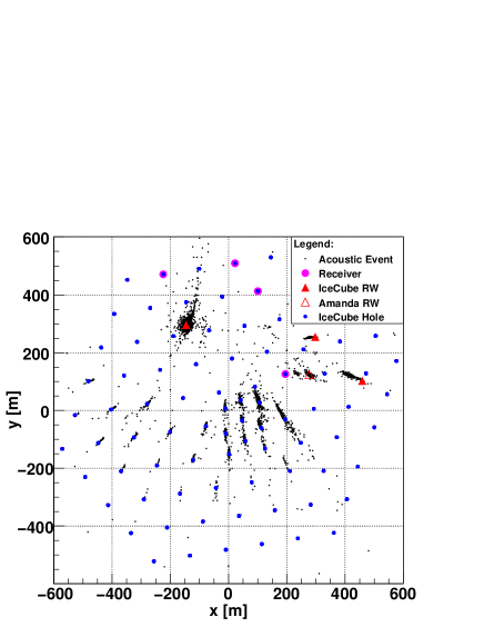
Figure 1: Horizontal distribution of all transient event vertices recorded since August 2008. The sources of transient noise are the Rodriguez Wells (RW), large caverns melted in the ice for water storage during IceCube drilling, and the re-freezing IceCube holes.

The recently used SPATS 12-channel configuration [7] allows statistical predictions by use of all possible sensor combinations per acoustic event. In case of a noise hit in a sensor the reconstruction algorithm for this combination does not converge or the result lies far outside the sensitive SPATS area. To improve the reconstruction result a cut at the tails of the vertex distribution of all sensor combinations has been applied. A horizontal distribution of all reconstructed transient events recorded since August 2008 is shown in Fig. 1.

2 Events from IceCube holes

Acoustic events were observed from nearly all IceCube holes drilled when transient data taking was active. The results for different holes are similar, therefore hole 81 is chosen below as an example.

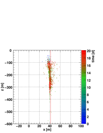
Figure 2: Events around the region of hole 81 between 10.12 till 31.12.2009 in the x-z plane. Visible are events before (firn drill), during and after (re-freezing) enhanced hot water drilling starts at the 20.12. The red line indicates the bore hole position.

Events are observed within 20 days in the hole region ($\pm 20$ m with respect to the center of hole 81) during the periods of firn ice drilling ($<50$ m depth), bulk ice drilling ($50-2500$ m depth) and re-freezing. Fig. 2 shows the depth position of the events versus the x-position, in chronological order. A few early events observed at 40 m - 100 m depth are connected with noise from the firn drill hole. During bulk ice drilling events are found in the same region but also at larger depth. Strong sound production starts about three days after drilling is finished, due to the refreezing process.

About 30 % of the registered events from this hole are concentrated in two spots at 120 m and 250 m depth but reaching down to about 600 m . The reason is that the hole doesn’t re-freeze homogeneously but forms frozen ice plugs between still water filled regions. The pressure produced in this way may give rise to cracks near the ice water boundary which appear with sound in the 10-100 kHz frequency region. Relaxation later continues within “arms” freezing upwards to the hole surface and down to the lower ice plug.
Besides providing information about the re-freezing process of water-filled IceCube holes one can use the corresponding acoustic events also to understand the precision of the vertex localization algorithm. The average values for the (x,y) position of hole 81 are determined to: 40.1$\pm$0.1 m in x and 39.4$\pm$0.1 m in y. The width of the distributions is 2.4 m and 4.6 m respectively to be compared with a hole diameter of about 70 cm. The calculated values deviate from the actual ones by 1.4 m (in x) and 3.9 m (in y). The possible reason for this deviation will be discussed in the simulation section 4 below.

3 Noise from Rodriguez-wells

When the first acoustic events had been reconstructed during the period from August to November 2008 (quiet period) a strong clustering in a certain region of the x-y plane at about (-150 m, 300 m) became visible. It was found that this was the position of the 2007/08 Rodriguez well (Rod-well or RW for short) used for the hot water drilling system.

This type of well has been introduced by Rodriguez and others in the early 1960s [2] for water supply at a glacier in Greenland. Hot water cycled by a pump system is used to melt ice below the firn layer at 60-80 m depth to maintain a fresh water reservoir. An expanding cavity is formed with a diameter as large as 15-20 m. For IceCube and its predecessor AMANDA this technique has been used in connection with drilling at the South Pole since mid 1990s. If the well is used a second time a year later, a second cavern is formed at a deeper level.

Having identified acoustic events arising from the 2007/08 Rod-well, three other event clusters were found, two of them could be attributed to other IceCube Rod-wells, from 2006/07 and 2004/05-2005/06. The fourth event cluster turned out to be located at the probable position of the last AMANDA Rod-well used in the final two drilling seasons up to 2001. No specific coordinates could, however, be found documented for that position anymore. The acoustic events from the Rod-wells used during two seasons are located at larger depths than those from Rod-wells used only once. The latter were seen to emit acoustic signals from smaller and smaller regions around the well core and finally stopped, the older one in October 2008, the younger one in May 2009.

In contrast to that, acoustic events are observed until today from the six and ten years old deeper wells (see Fig. 3). The mechanism of sound production in and around the Rod-well caverns is still under debate in particular for the older wells.

Table 1: Parameters of acoustic events from different Rod-wells.

Name	$x_{fit}[m]$	$y_{fit}[m]$	$z_{fit}[m]$	used	until
Amanda	$276.2\pm 0.4$	$123.6\pm 1.0$	$147.3\pm 1.1$	2y	now
IC 04-06	$412.6\pm 5.3$	$124.0\pm 2.4$	$147.8\pm 11.0$	2y	now
IC 06/07	$279.6\pm 0.4$	$252.2\pm 1.0$	$114.2\pm 0.7$	1y	Oct’08
IC 07/08	$-138.6\pm 0.4$	$297.7\pm 0.6$	$118.3\pm 1.0$	1y	May’09

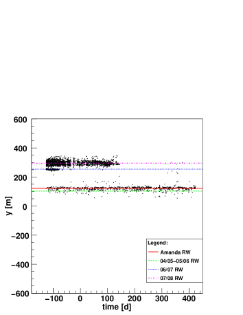
Figure 3: Acoustic events distribution for y-coordinate versus time. Lines: fitted positions of AMANDA-RW (red), 04/05-05/06 IC-RW (green), 06/07 IC-RW (blue), 07/08 IC-RW (magenta). The zero at the time axis indicates Jan 1, 2009.

4 Acoustic event simulation

A simple approach to acoustic transient event simulation can be done by calculating the signal propagation times for the distances $d_{n}=\sqrt{(x_{n}-x)^{2}+(y_{n}-y)^{2}+(z_{n}-z)^{2}}$ between source (e.g. IceCube hole at x,y,z) and sensors $n=1,...,n_{max}$ with $\Delta t_{n}=d_{n}/v_{s}$. The signal is randomly transmitted from a certain cylindrical volume (radius 2 m, depth 2000 m) around the source.

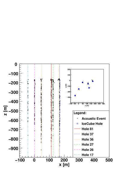
Figure 4: Reconstructed simulated events for visible holes of the drill season 08/09

Although knowing that the true IceCube hole diameter is about 70 cm, we take into account the possibility that tension cracks might appear outside the hole bounding surface which suggests a larger simulation radius. The reconstruction of events simulated with constant speed of sound and without considering attenuation effects implies an exact source localization, which is in contradiction to the real data vertex results, where a specific data spread around the source (Fig.1) and a lack of events below and above a certain depth (Fig.2) is visible. The major reason for misreconstruction of events at shallow depth (-200 m $<$ z $<$ 0 m) is probably the depth dependence of sound speed [3] which is, therefore, included in the simulation. Above 170 m depth, the parametrisation $v_{s}=-(262.379+199.833~{}|z|^{\frac{1}{2}}-1213.08~{}|z|^{\frac{1}{3}}){\rm ms^{-1}}$ and below a constant sound speed of $v_{s}=3850~{}{\rm ms^{-1}}$ is used. Further improvement is achieved using additional information on sound pressure wave attenuation in the ice [4]. We apply $S_{R}^{n}=(S_{0}\cdot d_{0}/d_{n})e^{-d_{n}/\lambda}$ with the initial amplitude $S_{0}$ at the distance $d_{0}$ chosen to fit the real data [5] and an attenuation length $\lambda$ of 300 m as measured for South Pole ice with SPATS [4]. If the signal strength at a sensor is above $\sim 300$ mV ($5.2~{}\sigma$ above the noise level) a hit is triggered as in real data.

A good agreement between reconstructed real and reconstructed simulated events is finally obtained as one can see by comparison of Fig.4 with Fig.1 and Fig.2. As expected we observe a large influence by the depth dependent sound speed on reconstructions in the upper region of SPATS (between 0 and 200 m depth). The significant deviation of the sound speed from the constant value used in the reconstruction explains the vertex spreading seen in the real data, whereas the direction of these “smearings” is caused by the detector geometry and points towards the center of SPATS. The inclusion of the attenuation length makes it more difficult to observe deep events which is in agreement with the real data distribution.

5 Noise from regions outside IceCube

In order to determine the number of events not connected to IceCube construction activities in the sensitive region of SPATS we omit the area of IceCube strings and the data-files from the drill periods keeping in mind that we have a lot of acoustic hits here due to detector construction. Furthermore we look at depths between 200 and 1000 m, in the region of constant speed of sound, to avoid the smearing described in section 4. In the 245 days of transient data taking we found no events for the recent SPATS-12 detector configuration in the region defined above which allows to determine a limit on the cosmogenic neutrino flux.

In order to determine a flux limit an effective volume for the SPATS-12 configuration is calculated. Neutrino interaction vertices were simulated in a cylindrical volume with an energy dependent sensitivity radius between $0.4-2~{}{\rm km}$ around the centre of SPATS and at depth between 200 and 1000 m. We omit again the area of IceCube strings. The neutrinos were assumed to be down going with random $\theta$ and $\phi$. Together with the interaction vertex, the direction ($\theta,\phi$) defines the plane of acoustic pressure wave. The sensor observation angle was then calculated relative to this plane for each vertex. $10^{7}$ events were simulated for neutrino energies $E_{\nu}$ increasing from $10^{18}{\rm eV}$ to $10^{22}{\rm eV}$. The hadronic component of the neutrino energy $E_{had}$ was assumed to be a constant fraction $y$ of the neutrino energy i.e. $E_{had}=0.2E_{\nu}$. In this simulation each acoustic sensor is simply a point at which to calculate the acoustic pressure $P_{max}$ as a function of $\theta$ and $R$. To get a reasonable value for the signal strength at the sensors we apply the Askaryan [6] model assuming a cylindrical energy deposition in the medium of length L and diameter d. No attempt has been made to model angular sensitivity or frequency response. A minimum threshold of $\sim$ 300 mV, like in the real SPATS-12 measurement is used, which transforms to a necessary minimum pressure of $\sim$ 70 mPa [7]. The observation of zero events inside the effective volume of SPATS-12 gives an upper limit of $N_{obs}=2.44$ events by a poissonian 90 % confidence level [8].

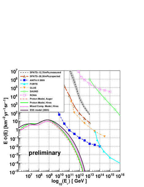
Figure 5: Neutrino flux limit of the recent SPATS configuration (70 mPa threshold, $\geq 5$ hits per events). The gray band (50-100 mPa threshold) around this limit considers uncertainties in absolute noise [7] and attenuation length [4].

The flux limit is shown in Fig.5 together with the cosmogenic neutrino flux predictions and results of other experiments. Additionally we show in Fig.5 the sensitivity for a SPATS-28 detector configuration which potentially would operate at a lower threshold of 30 mPa using a new detector readout.

References

- [1] R. Abbasi, et al., Background studies for acoustic neutrino detection at the South Pole, 2010, in preparation
- [2] R.P. Schmitt and R. Rodriguez, Glacier water supply and sewage disposal systems,Proceedings of the Symposium on Antarctic Logistics, Boulder, Colorado, 1962, National Academy of Sciences, National Research Council, 329-338.
- [3] R. Abbasi, et al., Measurement of sound speed vs depth in South Pole ice for neutrino astronomy, Astropart. Phys. 33 (2010) 277-286
- [4] R. Abbasi, et al., Measurement of Acoustic Attenuation in South Pole Ice, 2010, submitted to Astropart. Phys.
- [5] Juan-Pablo Yanez, Analysis of the acoustic attenuation length from transient signals in the South Pole ice, 2010, Master-Thesis Humboldt-Universität zu Berlin
- [6] G.Askaryan et al., Nucl. Instr. and Meth. A 164 (1979) 267.
- [7] T. Karg, Status and recent results of the South Pole Acoustic Test Setup, these proceedings.
- [8] G. J. Feldman and R. D. Cousins, Phys. Rev. D57 (1998) 3880 Table IV.