A Bregman Extension of quasi-Newton updates I:
An Information Geometrical framework

Abstract

We study quasi-Newton methods from the viewpoint of information geometry induced associated with Bregman divergences. Fletcher has studied a variational problem which derives the approximate Hessian update formula of the quasi-Newton methods. We point out that the variational problem is identical to optimization of the Kullback-Leibler divergence, which is a discrepancy measure between two probability distributions. The Kullback-Leibler divergence for the multinomial normal distribution corresponds to the objective function Fletcher has considered. We introduce the Bregman divergence as an extension of the Kullback-Leibler divergence, and derive extended quasi-Newton update formulae based on the variational problem with the Bregman divergence. As well as the Kullback-Leibler divergence, the Bregman divergence introduces the information geometrical structure on the set of positive definite matrices. From the geometrical viewpoint, we study the approximation Hessian update, the invariance property of the update formulae, and the sparse quasi-Newton methods. Especially, we point out that the sparse quasi-Newton method is closely related to statistical methods such as the EM-algorithm and the boosting algorithm. Information geometry is useful tool not only to better understand the quasi-Newton methods but also to design new update formulae.

1 Introduction

The main purpose of this article is to study the quasi-Newton methods from the view point of dualistic geometry or in other word information geometry [2, 26, 22]. Let us consider the unconstrained optimization problem

$$\text{minimize}\ f(x),\quad x\in\mathbb{R}^{n},$$ (1)

in which the function $f:\mathbb{R}^{n}\rightarrow\mathbb{R}$ is twice continuously differentiable on $\mathbb{R}^{n}$. The quasi-Newton method is known to be one of the most successful methods for unconstrained function optimization. In quasi-Newton method a sequence $\{x_{k}\}_{k=0}^{\infty}\subset\mathbb{R}^{n}$ is successively generated in a manner such that $x_{k+1}=x_{k}-\alpha_{k}B_{k}^{-1}\nabla f(x_{k})$, where $\alpha_{k}$ is a step length computed by a line search technique. The matrix $B_{k}$ is a positive definite matrix which is expected to approximate the Hessian matrix $\nabla^{2}f(x_{k})$. The matrix $B_{k}$ and the step length $\alpha_{k}$ are designed such that the sequence $x_{k}$ converges to a local minima of the problem (1). For the step length, the Wolfe condition [23, Section 3.1] is a standard criterion to determine the value of $\alpha_{k}$. In terms of the approximate Hessian matrix, mainly there are two methods of updating $B_{k}$ to $B_{k+1}$; one is called the DFP formula and the other is called the BFGS formula.

We introduce the DFP and the BFGS methods. Let $s_{k}$ and $y_{k}$ be column vectors defined by

$$s_{k}=x_{k+1}-x_{k}=-\alpha_{k}B_{k}^{-1}\nabla f(x_{k}),\qquad y_{k}=\nabla f(x_{k+1})-\nabla f(x_{k}),$$

and suppose that $s_{k}^{\top}y_{k}>0$ holds. In the DFP formula the approximate Hessian matrix $B_{k}$ is updated such that

$$B_{k+1} =B^{DFP}[B_{k};s_{k},y_{k}]:=B_{k}-\frac{B_{k}s_{k}y_{k}^{\top}+y_{k}s_{k}^{\top}B_{k}}{s_{k}^{\top}y_{k}}+s_{k}^{\top}B_{k}s_{k}\frac{y_{k}y_{k}^{\top}}{(s_{k}^{\top}y_{k})^{2}}+\frac{y_{k}y_{k}^{\top}}{s_{k}^{\top}y_{k}}.$$ (2)

In the BFGS update formula, the matrix $B_{k+1}$ is defined by

$$B_{k+1} =B^{BFGS}[B_{k};s_{k},y_{k}]:=B_{k}-\frac{B_{k}s_{k}s_{k}^{\top}B_{k}}{s_{k}^{\top}B_{k}s_{k}}+\frac{y_{k}y_{k}^{\top}}{s_{k}^{\top}y_{k}},$$ (3)

Under the condition that $B_{k}\in\mathrm{PD}(n)$ and $s_{k}^{\top}y_{k}>0$, the matrices $B^{DFP}[B_{k};s_{k},y_{k}]$ and $B^{BFGS}[B_{k};s_{k},y_{k}]$ are also positive definite matrices. If there is no confusion, the update formulae $B^{DFP}[B;s,y]$ and $B^{BFGS}[B;s,y]$ are written as $B^{DFP}[B]$ and $B^{BFGS}[B]$, respectively. In practice, the Cholesky decomposition of $B_{k}$ is successively updated in order to compute the search direction $-B_{k}^{-1}\nabla f(x_{k})$ efficiently [14]. Note that the equality

$$B^{DFP}[B;s,y]^{-1}=B^{BFGS}[B^{-1};y,s]$$

holds. Hence, we can derive the update formulae for the inverse $H_{k}=B_{k}^{-1}$ without inversion of matrix.

Both the DFP and the BFGS methods are derived from variational problems over the set of positive definite matrices [10]. Let $\mathrm{PD}(n)$ be the set of all $n$ by $n$ symmetric positive definite matrices, and the function $\psi:\mathrm{PD}(n)\rightarrow\mathbb{R}$ be a strictly convex function over $\mathrm{PD}(n)$ defined by

$$\psi(A)={\mathrm{tr}(A)}-\log\det{A}.$$

Fletcher [10] has shown that the DFP update formula (2) is obtained as the unique solution of the constraint optimization problem,

$$\min_{B\in\mathrm{PD}(n)}\ \psi(B_{k}^{1/2}B^{-1}B_{k}^{1/2})\quad\text{\rm subject to }\ Bs_{k}=y_{k},$$

where $A^{1/2}$ for $A\in\mathrm{PD}(n)$ is the matrix satisfying $A^{1/2}\in\mathrm{PD}(n)$ and $(A^{1/2})^{2}=A$. The BFGS formula is also obtained as the optimal solution of

$$\min_{B\in\mathrm{PD}(n)}\ \psi(B_{k}^{-1/2}BB_{k}^{-1/2})\quad\text{\rm subject to }\ Bs_{k}=y_{k},$$

in which $B_{k}^{-1/2}$ denotes $(B_{k}^{-1})^{1/2}$ or equivalently $(B_{k}^{1/2})^{-1}$.

It will be worthwhile to point out that the function $\psi$ is identical to Kullback-Leibler(KL) divergence [2, 19] up to an additive constant. For $P,Q\in\mathrm{PD}(n)$, the KL-divergence is defined by

$$\mathrm{KL}(P,Q) ={\mathrm{tr}(PQ^{-1})}-\log\det(PQ^{-1})-n$$

which is equal to $\psi(Q^{-1/2}PQ^{-1/2})-n$. The KL-divergence is regarded as a generalization of squared distance. Using the KL-divergence, we can represent the update formulae as the optimal solutions of the following minimization problems,

(DFP) $$\min_{B\in\mathrm{PD}(n)}\ \mathrm{KL}(B_{k},B)\quad\text{\rm subject to }\ Bs_{k}=y_{k},$$ (4)

(BFGS) $$\min_{B\in\mathrm{PD}(n)}\ \mathrm{KL}(B,B_{k})\quad\text{\rm subject to }\ Bs_{k}=y_{k}.$$ (5)

The KL-divergence is asymmetric, that is, $\mathrm{KL}(P,Q)\neq\mathrm{KL}(Q,P)$ in general. Hence the above problems will provide different solutions.

In the information geometry [2], the KL-divergence defines a geometrical structure over the space of probability densities. Statistical inference such that the maximum likelihood estimator is better understood based on the geometrical intuition. Originally, the KL-divergence is defined as the discrepancy measure between two multinomial normal distributions with mean zero. In this paper, we show that the information geometrical approach is useful to understand the behaviour of quasi-Newton methods. On the set of positive definite matrices, $\mathrm{PD}(n)$, we define the so-called Bregman divergence which is an extension of the KL-divergence. The Bregman divergence induces a dualistic geometrical structure on $\mathrm{PD}(n)$. Then we can derive new Hessian update formulae based on the Bregman divergence. We present a geometrical view of quasi-Newton updates, and discuss the relation between the Hessian update formula and the statistical inference based on the information geometry.

Here is the brief outline of the article. In Section 2, we introduce the elements of information geometry based on the Bregman divergence, especially over the set of positive definite matrices. In Section 3, an extended quasi-Newton formula is derived from the Bregman divergence. Section 4 is devoted to discuss the invariance property of the quasi-Newton update formula under the group action. In Section 5, we discuss the sparse quasi-Newton methods [32] from the viewpoint of the information geometry, and point out that the sparse quasi-Newton method is closely related to statistical methods such as the EM-algorithm [20] or the boosting algorithm [12, 22]. We conclude with a discussion and outlook in Section 6. Some proofs of the theorems are postponed to Appendix.

Throughout the paper, we use the following notations: The set of positive real numbers are denoted as $\mathbb{R}_{+}\subset\mathbb{R}$. Let $\det{A}$ be the determinant of square matrix $A$, and $\mathrm{GL}(n)$ denotes the set of $n$ by $n$ non-degenerate real matrices. $\mathrm{SL}(n)\subset\mathrm{GL}(n)$ is the set of $n$ by $n$ non-degenerate real matrices with determinant $1$, that is, $\mathrm{SL}(n)=\{A\in\mathrm{GL}(n)~{}|~{}\det{A}=1\}$. The set of all $n$ by $n$ real symmetric matrices is denoted as $\mathrm{Sym}(n)$, and let $\mathrm{PD}(n)\subset\mathrm{GL}(n)\cap\mathrm{Sym}(n)$ be the set of $n$ by $n$ symmetric positive definite matrices. For $P\in\mathrm{PD}(n)$, the square root of $P$ is denoted as $P^{1/2}$ which is defined as $P$ For a vector $x$, $\|x\|$ denotes the Euclidean norm. For two square matrices $A,\,B$, the inner product $\langle A,B\rangle$ is defined by ${\mathrm{tr}(AB^{\top})}$, and $\|A\|_{F}$ is the Frobenius norm defined by the square root of $\langle A,A\rangle$. Throughout the paper we only deal with the inner product of symmetric matrices, and the transposition in the trace can be dropped.

2 Bregman Divergences and Dualistic Geometry of Positive Definite Matrices

We introduce Bregman divergences which are regarded as an extension of the KL-divergence. Then we illustrate a differential geometrical structure defined from the Bregman divergence over the set of positive definite matrices. In sequel sections, we will provide a geometrical interpretation of quasi-Newton methods. For general Bregman divergences, however, the quasi-Newton update formula cannot be obtained in the explicit form. In order to obtain computationally tractable update formulae, we often use a specific Bregman divergence which is called the $V$-Bregman divergence in this article. First, we define general Bregman divergences, and then we introduce the $V$-Bregman divergence as a special case of general Bregman divergences. We will show the associated geometrical structure on the set of positive definite matrices.

2.1 Bregman divergences

The Bregman divergence [7] is defined through the so-called potential function. Below, we define the Bregman divergence over the set of positive definite matrices.

Definition 1 (Potential function and Bregman divergence).

Let $\varphi:\mathrm{PD}(n)\rightarrow\mathbb{R}$ be a continuously differentiable, strictly convex function that maps positive definite matrices to real numbers. The function $\varphi$ is referred to as potential function or potential for short. Given a potential $\varphi$, the Bregman divergence $D_{\varphi}(P,Q)$ is defined as

$$D_{\varphi}(P,Q)=\varphi(P)-\varphi(Q)-\langle\nabla\varphi(Q),P-Q\rangle$$ (6)

for $P,Q\in\mathrm{PD}(n)$, where $\nabla\varphi(Q)$ is the $n$ by $n$ matrix whose $(i,j)$ element is given as $\frac{\partial\varphi}{\partial Q_{ij}}(Q)$.

The Bregman divergence $D_{\varphi}(P,Q)$ is non-negative and equals zero if and only if $P=Q$ holds. Indeed, due to the strict convexity of $\varphi$, the function $\varphi(P)$ lies above its tangents $\varphi(Q)+\langle\nabla\varphi(Q),P-Q\rangle$ at $Q$. Hence, the non-negativity of the Bregman divergence $D_{\varphi}(P,Q)$ is guaranteed. Note that $D_{\varphi}(P,Q)$ is convex in $P$ but not necessarily convex in $Q$. Bregman divergences have been well studied in the fields of statistics and machine learning [3, 9, 22].

Example 1.

For $P\in\mathrm{PD}(n)$ let the function $\varphi$ be $\varphi(P)=-\log\det(P)$. Note that $\varphi(P)$ is a strictly convex function. Then, we have

$$(\nabla\varphi(Q))_{ij}=-\frac{\partial}{\partial Q_{ij}}\log\det Q=-(Q^{-1})_{ji}.$$

Hence the corresponding Bregman divergence is

$$D_{\varphi}(P,Q)=-\log\det{P}+\log\det{Q}+\langle Q^{-1},P-Q\rangle=\langle P,Q^{-1}\rangle-\log\det(PQ^{-1})-n,$$

is identical to the KL-divergence on the multivariate normal distribution with mean zero [2, 27].

By replacing the KL-divergence in (4) or (5) with a Bregman divergence, we will obtain another variational problem for the quasi-Newton method. In general, however, update formula cannot be explicitly obtained. Below we define a class of Bregman divergences called $V$-Bregman divergence. In Section 3, we show that the $V$-Bregman divergence provides an explicit update formula of the quasi-Newton method.

We prepare some ingredients to define the $V$-Bregman divergence. Let $V:\mathbb{R}_{+}\rightarrow\mathbb{R}$ be a strictly convex, decreasing, and third order continuously differentiable function. For the derivative $V^{\prime}$, the inequality $V^{\prime}<0$ holds from the condition. Indeed, the condition leads to $V^{\prime}\leq 0$ and $V^{\prime\prime}\geq 0$, and if $V^{\prime}(z_{0})=0$ holds for some $z_{0}\in\mathbb{R}_{+}$, then $V^{\prime}(z)=0$ holds for all $z\geq z_{0}$. Hence $V(z)$ is affine function for $z\geq z_{0}$. This contradicts the strict convexity of $V$. We define the functions $\nu_{V}:\mathbb{R}_{+}\rightarrow\mathbb{R}$ and $\beta_{V}:\mathbb{R}_{+}\rightarrow\mathbb{R}$ such that

$$\nu_{V}(z)=-zV^{\prime}(z),\qquad\beta_{V}(z)=\frac{z\nu_{V}^{\prime}(z)}{\nu_{V}(z)}=z\cdot\frac{d}{dz}\log\nu_{V}(z)$$

Since $\nu_{V}(z)>0$ holds for $z>0$, the function $\beta_{V}$ is well defined on $\mathbb{R}_{+}$. The subscript $V$ of $\nu_{V}$ and $\beta_{V}$ will be dropped if there is no confusion. We now are ready to present the definition of $V$-Bregman divergence over $\mathrm{PD}(n)$.

Definition 2 ($V$-Bregman divergence).

Let $V:\mathbb{R}_{+}\rightarrow\mathbb{R}$ be a function which is strictly convex, decreasing, and third order continuously differentiable. Suppose that the functions $\nu$ and $\beta$ defined from $V$ satisfy the following conditions:

$$\beta(z)<\frac{1}{n}\qquad(z>0)$$ (7)

and

$$\lim_{z\rightarrow+0}\frac{z}{\nu(z)^{n-1}}=0.$$ (8)

The Bregman divergence defined from the potential $\varphi(P)=V(\det{P})$ is called $V$-Bregman divergence, and denoted as $D_{V}(P,Q)$. Not only $V(\det{P})$ but also $V(z)$ is also referred to as potential.

As shown in [26], the function $V(\det{P})$ is strictly convex in $P\in\mathrm{PD}(n)$ if and only if the potential $V$ satisfies (7). The $V$-Bregman divergence has the form of

$$D_{V}(P,Q)=V(\det{P})-V(\det{Q})+\nu(\det{Q})\langle Q^{-1},P\rangle-n\nu(\det{Q}).$$ (9)

Indeed, substituting

$$(\nabla\varphi(Q))_{ij}=\frac{\partial V(\det{Q})}{\partial Q_{ij}}=V^{\prime}(\det{Q})\frac{\partial\det{Q}}{\partial Q_{ij}}=-\nu(\det{Q})(Q^{-1})_{ij},$$

into (6), we obtain the expression of $D_{V}(P,Q)$. The KL-divergence $\mathrm{KL}(P,Q)$ is represented as $D_{V}(P,Q)$ with the potential $V(z)=-\log z$. Below we show some examples of $V$-Bregman divergence.

Example 2.

For the power potential $V(z)=(1-z^{\gamma})/\gamma$ with $\gamma<1/n$, we have $\nu(z)=z^{\gamma}$ and $\beta(z)=\gamma$. Then, we obtain

$$D_{V}(P,Q)=(\det{Q})^{\gamma}\bigg{\{}\langle P,Q^{-1}\rangle+\frac{1-(\det{PQ^{-1}})^{\gamma}}{\gamma}-n\bigg{\}}.$$

The KL-divergence is recovered by taking the limit of $\gamma\rightarrow 0$.

Example 3.

For $0\leq c<1$, let us define $V(z)=c\log(cz+1)-\log(z)$. Then $V(z)$ is a strictly convex and decreasing function, and we obtain

$$\nu(z)=1-c+\frac{c}{cz+1}>0,\qquad\beta(z)=\frac{-c^{2}z}{(cz+1)(c(1-c)z+1)}\leq 0$$

for $z>0$. The negative-log potential, $V(z)=-\log z$, is recovered by setting $c=0$. The potential satisfies the bounding condition $0<1-c\leq\nu(z)\leq 1$. As shown in the sequel [17], the bounding condition of $\nu$ will be assumed to prove the convergence property of the quasi-Newton method.

2.2 Dualistic Geometry defined from Bregman Divergences

The space of positive definite matrices has rich geometrical and algebraic structures [26] Here we introduce dualistic geometrical structure on $\mathrm{PD}(n)$ induced form the Bregman divergence. See [22, 25] for details.

We introduce two coordinate systems on $\mathrm{PD}(n)$. The $\eta$-coordinate system $\eta:\mathrm{PD}(n)\rightarrow\mathrm{PD}(n)$ is defined as

$$\eta(P)=P,$$

which is the identity function on $\mathrm{PD}(n)$. The definition of the other coordinate system requires the potential $\varphi$ for the Bregman divergence $D_{\varphi}(P,Q)$ in (6). Let us define the $\theta_{\varphi}$-coordinate system as

$$\theta_{\varphi}(P)=\nabla\varphi(P)$$

Note that the matrix $\theta_{\varphi}(P)$ is not necessarily a positive definite matrix. Indeed, for the potential $\varphi(P)=-\log\det P$, we have $\theta_{\varphi}(P)=-P^{-1}$ which is a negative definite matrix. The function $\theta_{\varphi}$ is, however, one-to-one mapping. Hence $\theta_{\varphi}(P)$ works as the coordinate system on $\mathrm{PD}(n)$. The inverse function of $\nabla\varphi$ is expressed by the conjugate function of $\varphi$. The convex function $\varphi$ has the dual representation called Fenchel conjugate, which is defined as

$$\varphi^{*}(P)=\sup_{Q\in\mathrm{PD}(n)}\big{\{}\langle P,Q\rangle-\varphi(Q)\big{\}}.$$ (10)

Then, we have

$$\nabla\varphi^{*}(P)=(\nabla\varphi)^{-1}(P)=(\theta_{\varphi})^{-1}(P)$$

on the domain of $\varphi^{*}$ [30, Theorem 26.5]. For any potential $\varphi$, the $\eta$-coordinate system is common and only the $\theta_{\varphi}$-coordinate system depends on the potential.

For the potential $V$ of the $V$-Bregman divergence, the $\theta_{\varphi}$-coordinate system is denoted as $\theta_{V}(P)$, which is given as

$$\theta_{V}(P)=-\nu(P)P^{-1}.$$

Thus $\theta_{V}(P)$ is a negative definite matrix for $P\in\mathrm{PD}(n)$.

Let us define the flatness of a submanifold in $\mathrm{PD}(n)$. See [2] for the formal definition of the flatness with terminologies of differential geometry.

Definition 3 (autoparallel submanifold).

Let $\mathcal{M}$ be a subset of $\mathrm{PD}(n)$. If $\mathcal{M}$ is represented as an affine subspace in the $\eta$-coordinate, then $\mathcal{M}$ is called $\eta$-autoparallel submanifold. If $\mathcal{M}$ is represented as an affine subspace in the $\theta_{\varphi}$-coordinate, then $\mathcal{M}$ is called $\theta_{\varphi}$-autoparallel submanifold. When an $\eta$-autoparallel submanifold $\mathcal{M}$ is also $\theta_{\varphi}$-autoparallel, $\mathcal{M}$ is called doubly autoparallel submanifold.

For the potential $\varphi(P)=V(\det{P})$, the $\theta_{\varphi}$-coordinate and the $\theta_{\varphi}$-autoparallel is denoted as the $\theta_{V}$-coordinate and the $\theta_{V}$-autoparallel, respectively. Formally, the flatness is defined from the connection on the differentiable manifold [2, 18]. Here, we adopt a simplified definition.

Example 4.

Let $V(z)$ be the negative logarithmic function $V(z)=-\log(z)$, then we have $\nu(z)=1$. The $\eta$-coordinate system is defined as $\eta(P)=P$, and the $\theta_{V}$-coordinate system is given as $\theta_{V}(P)=-P^{-1}$. For two vectors $s,\,y\in\mathbb{R}^{n}$ we define the submanifold $\mathcal{M}$ which represents the secant condition such that

$$\mathcal{M}=\{B\in\mathrm{PD}(n)~{}|~{}Bs=y\}.$$

Suppose $\mathcal{M}\neq\emptyset$, then we see that $\mathcal{M}$ is doubly autoparallel, since

$$\mathcal{M}=\{B\in\mathrm{PD}(n)\,|\,\eta(B)s=y\}=\{B\in\mathrm{PD}(n)\,|\,\theta_{V}(B)y=-s\}$$

holds. That is, $\mathcal{M}$ is represented as the affine subspace in both the $\eta$-coordinate system and the $\theta_{V}$-coordinate system.

2.3 Extended Pythagorean Theorem

The projection of a matrix in $\mathrm{PD}(n)$ onto an autoparallel submanifold is defined below. Then, we introduce the extended Pythagorean theorem.

Definition 4 (projection).

Let $\varphi$ be a potential, $Q$ be a positive definite matrix. An $\eta$-autoparallel submanifold in $\mathrm{PD}(n)$ is denoted as $\mathcal{M}$. The matrix $P^{*}\in\mathcal{M}$ is called $\theta_{\varphi}$-projection of $Q$ onto $\mathcal{M}$, when the equality

$$\langle\theta_{\varphi}(Q)-\theta_{\varphi}(P^{*}),\,\eta(P)-\eta(P^{*})\rangle=0,\quad^{\forall}P\in\mathcal{M}$$

holds. Let $\mathcal{N}$ be a $\theta_{\varphi}$-autoparallel submanifold in $\mathrm{PD}(n)$. The matrix $P^{*}\in\mathcal{N}$ is called $\eta$-projection of $Q$ onto $\mathcal{N}$ when the equality

$$\langle\eta(Q)-\eta(P^{*}),\,\theta_{\varphi}(P)-\theta_{\varphi}(P^{*})\rangle=0,\quad^{\forall}P\in\mathcal{N}$$

holds.

Let $\mathcal{L}$ be a one-dimensional $\theta_{\varphi}$-autoparallel submanifold defined as

$$\mathcal{L}=\big{\{}P\in\mathrm{PD}(n)\,|\,^{\exists}t\in\mathbb{R},\ \theta_{\varphi}(P)=(1-t)\theta_{\varphi}(Q)+t\theta_{\varphi}(P^{*})\big{\}}.$$

When $P^{*}$ is the $\theta_{\varphi}$-projection of $Q$ onto $\mathcal{M}$, the $\eta$-autoparallel submanifold $\mathcal{M}$ is orthogonal to $\mathcal{L}$ at $P^{*}$ with respect to the inner product $\langle\cdot\,,\cdot\rangle$. In the $\eta$-projection, also the same picture holds by replacing $\eta$ and $\theta_{\varphi}$.

Theorem 1 (Extended Pythagorean Theorem [2, 22]).

Let $\varphi$ be a potential function, $\mathcal{M}$ be an $\eta$-autoparallel submanifold in $\mathrm{PD}(n)$, and $Q$ be a positive definite matrix. Then, the following three statements are equivalent.

(a)

$P^{*}$ is a $\theta_{\varphi}$-projection of $Q$ onto $\mathcal{M}$.

(b)

$P^{*}\in\mathcal{M}$ satisfies the equality

$$D_{\varphi}(P,Q)=D_{\varphi}(P,P^{*})+D_{\varphi}(P^{*},Q)$$ (11)

for any $P\in\mathcal{M}$.

(c)

$P^{*}$ is the unique optimal solution of the problem

$$\min_{P\in\mathrm{PD}(n)}\,D_{\varphi}(P,Q)\quad\text{\rm subject to }P\in\mathcal{M}.$$ (12)

Proof.

For any $P,P^{*},Q\in\mathrm{PD}(n)$ the equality

$$D_{\varphi}(P,Q)-D_{\varphi}(P,P^{*})-D_{\varphi}(P^{*},Q)=\langle\theta_{\varphi}(Q)-\theta_{\varphi}(P^{*}),\,\eta(P^{*})-\eta(P)\rangle$$ (13)

holds. The equivalence between (a) and (b) follows the above equality. If (b) holds, then the non-negativity of the divergence assures that $P^{*}$ is an optimal solution of (12). The uniqueness follows the strict convexity of the divergence $D_{\varphi}(P,Q)$ in $P$. Hence (c) holds. Finally, we show that (a) follows (c). Let $P^{*}$ be an optimal solution of (12). The $\eta$-autoparallel submanifold $\mathcal{M}$ is represented by

$$\mathcal{M} =\{P\in\mathrm{PD}(n)~{}|~{}\langle\eta(P),A_{i}\rangle=b_{i},\,i=1,\ldots,k\}$$

in which $A_{i}$ is an $n$ by $n$ real matrix and $b_{i}\in\mathbb{R}$ for $i=1,\ldots,k$. The optimality condition of (12) yields that

$$-\theta_{\varphi}(P^{*})+\theta_{\varphi}(Q)=\sum_{i=1}^{k}\lambda_{i}A_{i},\quad\lambda_{i}\in\mathbb{R}$$

with some $\lambda_{1},\ldots,\lambda_{k}$. In addition, the fact that both $P$ and $P^{*}$ are included in $\mathcal{M}$ leads to the equalities

$$\langle\eta(P^{*})-\eta(P),A_{i}\rangle=0,\quad i=1,\ldots,k.$$

Therefore, we obtain

$$\langle\theta_{\varphi}(Q)-\theta_{\varphi}(P^{*}),\eta(P^{*})-\eta(P)\rangle=0$$

for any $P\in\mathcal{M}$. This implies that $P^{*}$ is a $\theta_{\varphi}$-projection of $Q$ onto $\mathcal{M}$. $\Box$

The uniqueness of the $\theta_{\varphi}$-projection onto the $\eta$-autoparallel submanifold is shown through the equivalence between (a) and (b) in Theorem 1. The similar argument is valid for $\eta$-projection onto $\theta_{\varphi}$-autoparallel submanifold. We show the result without proof.

Theorem 2.

Let $\varphi$ be a potential function, $\mathcal{N}$ be a $\theta_{\varphi}$-autoparallel submanifold in $\mathrm{PD}(n)$, and $Q$ be a positive definite matrix. Then, the following conditions (a) and (b) are equivalent.

(a)

$P^{*}$ is an $\eta$-projection of $Q$ onto $\mathcal{N}$.

(b)

$P^{*}\in\mathcal{N}$ satisfies the equality

$$D_{\varphi}(Q,P)=D_{\varphi}(Q,P^{*})+D_{\varphi}(P^{*},P)$$ (14)

for any $P\in\mathcal{N}$.

When (a) or (b) holds, $P^{*}$ is the unique optimal solution of the problem

$$\min_{P\in\mathrm{PD}(n)}\,D_{\varphi}(Q,P)\quad\text{\rm subject to }P\in\mathcal{N}.$$ (15)

The Bregman divergence $D_{\varphi}(Q,P)$ may not be convex in $P$, and hence the conditions (a) or (b) in Theorem (2) is not necessarily derived from the optimality condition of (15).

As shown in Section 1, the BFGS/DFP update formulae are derived by minimizing the KL-divergence. Example 4 shows that the submanifold associated with the secant condition $\mathcal{M}=\{B\in\mathrm{PD}(n)~{}|~{}Bs_{k}=y_{k}\}$ is doubly autoparallel with respect to the flatness defined from the potential $V(z)=-\log z$. Thus, we obtain the following geometrical interpretation,

BFGS update:

$\theta_{V}$-projection of $B_{k}$ onto the $\eta$-autoparallel submanifold $\mathcal{M}$,

DFP update:

$\eta$-projection of $B_{k}$ onto the $\theta_{V}$-autoparallel submanifold $\mathcal{M}$.

Figure 1 presents the geometrical view of the standard quasi-Newton updates based on information geometry.

Figure 1: Geometrical interpretation of quasi-Newton updates. For the potential $V(z)=-\log z$, the submanifold $\mathcal{M}$ defined by the secant condition is doubly autoparallel with respect to $\eta$- and $\theta_{V}$-coordinate systems. The BFGS formula $B^{\mathrm{BFGS}}[B_{k}]$ is given as the $\theta_{V}$-projection of $B_{k}$ onto the $\eta$-autoparallel submanifold $\mathcal{M}$, and the DFP update $B^{\mathrm{DFP}}[B_{k}]$ is given as the $\eta$-projection of $B_{k}$ onto the $\theta_{V}$-autoparallel submanifold $\mathcal{M}$.

3 quasi-Newton Methods based on Bregman Divergences

We consider quasi-Newton update formulae derived from variational problems with respect to Bregman divergences. As shown in Section 1, the standard quasi-Newton updates are derived from the minimization problem of the KL-divergence. We show that Bregman divergences lead extended update formulae. In addition, an explicit expression of the extended Hessian update formula is presented.

We consider the minimization problem of the Bregman divergence instead of the KL-divergence. The extended BFGS update formula is given as the optimal solution of

$$\min_{B\in\mathrm{PD}(n)}\ D_{\varphi}(B,B_{k}),\quad\text{subject to}\ \ Bs_{k}=y_{k}.$$ (16)

Suppose that the optimal solution $B_{k+1}$ exists. Then $B_{k+1}$ is the unique $\theta_{\varphi}$-projection of $B_{k}$ onto the submanifold defined from the secant condition. On the other hand, as the extension of the DFP update, we consider the problem,

$$\min_{B\in\mathrm{PD}(n)}\ D_{\varphi}(B^{-1},B_{k}^{-1}),\quad\text{subject to}\ \ Bs_{k}=y_{k}.$$ (17)

instead of the minimization of $\mathrm{KL}(B_{k},B)=\mathrm{KL}(B^{-1},B_{k}^{-1})$. In the similar way, we can derive the quasi-Newton methods for the approximate inverse Hessian matrix $H_{k}=B_{k}^{-1}$.

In the following we focus on the extension of the BFGS method (16), since the same argument is valid for the extension of DFP method. A formal expression of the optimal solution is presented in the theorem below.

Theorem 3.

Suppose that there exists an optimal solution (16). Then the optimal solution $B_{k+1}$ is unique and satisfies

$$B_{k+1}=\nabla\varphi^{*}\big{(}\nabla\varphi(B_{k})+s_{k}\lambda^{\top}+\lambda s_{k}^{\top}\big{)},\qquad B_{k+1}s_{k}=y_{k},$$

where $\lambda\in\mathbb{R}^{n}$ is a column vector and $\varphi^{*}$ is the Fenchel conjugate function of $\varphi$.

Proof.

Since (16) is a convex problem and the objective function $D_{\varphi}(B,B_{k})$ is strictly convex in $B$, we see that the optimal solution is unique if it exists. Suppose that $B_{k+1}$ is the optimal solution of (16), then $B_{k+1}$ satisfies the optimality condition. According to Güler, et al. [16], the normal vector of the affine subspace $\mathcal{M}=\{B\in\mathrm{PD}(n)~{}|~{}Bs_{k}=y_{k}\}$ is characterized by the form of

$$s_{k}\lambda^{\top}+\lambda s_{k}^{\top}\in\mathrm{Sym}(n),\qquad\lambda\in\mathbb{R}^{n}.$$

In fact for $B_{1},B_{2}\in\mathcal{M}$ we have

$$\langle s_{k}\lambda^{\top}+\lambda s_{k}^{\top},\,B_{1}-B_{2}\rangle =\lambda^{\top}B_{1}s_{k}+s_{k}^{\top}B_{1}\lambda-\lambda^{\top}B_{2}s_{k}-s_{k}^{\top}B_{2}\lambda$$

$$=\lambda^{\top}y_{k}+y_{k}^{\top}\lambda-\lambda^{\top}y_{k}-y_{k}^{\top}\lambda$$

$$=0,$$

and thus $s_{k}\lambda^{\top}+\lambda s_{k}^{\top}$ is a normal vector of $\mathcal{M}$. Güler, et al. [16] have shown that the normal vector is restricted to the expression above. Hence, for the optimal solution $B_{k+1}$ there exists $\lambda\in\mathbb{R}^{n}$ such that $\nabla D_{\varphi}(B,B_{k})\big{|}_{B=B_{k+1}}=s_{k}\lambda^{\top}+\lambda s_{k}^{\top}$ and $B_{k}s_{k}=y_{k}$ hold. The first equality is represented as $\nabla\varphi(B_{k+1})-\nabla\varphi(B_{k})=s_{k}\lambda^{\top}+\lambda s_{k}^{\top}$. The existence of $B_{k+1}$ assures that $B_{k+1}=\nabla\varphi^{*}\big{(}\nabla\varphi(B_{k})+s_{k}\lambda^{\top}+\lambda s_{k}^{\top}\big{)}$, where $\varphi^{*}$ is the Fenchel conjugate of $\varphi$ defined in (10). $\Box$

For general Bregman divergences, we do not have the explicit expression of the Hessian update formula. As a special case, we consider the minimization problem of the $V$-Bregman divergence,

$$\text{$V$-BFGS:}\qquad\min_{B\in\mathrm{PD}(n)}\ D_{V}(B,B_{k}),\quad\text{subject to}\ \ Bs_{k}=y_{k}.$$ (18)

The update formula obtained by the problem above is referred to as the $V$-BFGS update formula. The theorem below shows an explicit expression of the $V$-BFGS update formula.

Theorem 4 ($V$-BFGS update formula).

Suppose the function $V$ is a potential function defined in Definition 2. Let $B_{k}\in\mathrm{PD}(n)$, and suppose $s_{k}^{\top}y_{k}>0$. Then the problem (18) has the unique optimal solution $B_{k+1}\in\mathrm{PD}(n)$ satisfying

$$B_{k+1} =\frac{\nu(\det{B_{k+1}})}{\nu(\det{B_{k}})}B^{BFGS}[B_{k};s_{k},y_{k}]+\bigg{(}1-\frac{\nu(\det{B_{k+1}})}{\nu(\det{B_{k}})}\bigg{)}\frac{y_{k}y_{k}^{\top}}{s_{k}^{\top}y_{k}}.$$ (19)

Though the theorem is proved in [17], the proof is also found in Appendix A of the present paper as a supplementary. In the same way, we can obtain the explicit formula of the $V$-DFP update formula, which is the minimizer of $D_{V}(B^{-1},B_{k}^{-1})$ subject to $Bs_{k}=y_{k}$. The update formula is equivalent to the self-scaling quasi-Newton update defined as

$$B_{k+1} =\theta_{k}B^{BFGS}[B_{k};s_{k},y_{k}]+(1-\theta_{k})\frac{y_{k}y_{k}^{\top}}{s_{k}^{\top}y_{k}},$$ (20)

where $\theta_{k}$ is a positive real number. Various choices for $\theta_{k}$ have been proposed, see [29, 24]. A popular choice is $\theta_{k}=s_{k}^{\top}y_{k}/s_{k}^{\top}B_{k}s_{k}$. In the $V$-BFGS update formula, the coefficient $\theta_{k}$ is determined from the function $\nu$.

We present a practical way of computing the Hessian approximation (19). Details are shown in the sequel [17]. In Eq (19), the optimal solution $B_{k+1}$ appears in both sides, that is, we have only the implicit expression of $B_{k+1}$. The numerical computation is, however, efficiently conducted as well as the standard BFGS update. To compute the matrix $B_{k+1}$, first we compute the determinant $\det B_{k+1}$. The determinant of both sides of (19) leads to

$$\det B_{k+1}=\frac{\det(B^{BFGS}[B_{k};s_{k},y_{k}])}{\nu(\det B_{k})^{n-1}}\cdot\nu(\det B_{k+1})^{n-1}.$$ (21)

Hence, by solving the nonlinear equation

$$z=\frac{\det(B^{BFGS}[B_{k};s_{k},y_{k}])}{\nu(\det B_{k})^{n-1}}\cdot\nu(z)^{n-1},\qquad z>0$$

we can find $\det B_{k+1}$. As shown in the proof of Theorem 4, the function $z/\nu(z)^{n-1}$ is monotone increasing. Hence the Newton method is available to find the root of the above equation efficiently. Once we obtain the value of $\det B_{k+1}$, we can compute the Hessian approximation $B_{k+1}$ by substituting $\det B_{k+1}$ into Eq (19). Figure 2 shows the update algorithm of the $V$-BFGS formula which exploits the Cholesky decomposition of the approximate Hessian matrix. By maintaining the Cholesky decomposition, we can easily compute the the determinant and the search direction. The convergence property of the quasi-Newton method with the $V$-BFGS update formula is considered in [17].

$V$-BFGS update: Initialization: The function $\nu(z)$ denotes $-V^{\prime}(z)z$. Let $B_{0}\in\mathrm{PD}(n)$ be a matrix which is an initial approximation of the Hessian matrix, and $L_{0}L_{0}^{\top}=B_{0}$ be the Cholesky decomposition of $B_{0}$. Let $x_{0}\in\mathbb{R}^{n}$ be an initial point, and set $k=0$. Repeat: If stopping criterion is satisfied, go to Output. 1. Let $x_{k+1}=x_{k}-\alpha_{k}B_{k}^{-1}\nabla f(x_{k})$, where $\alpha_{k}\geq 0$ is a step length satisfying the Wolfe condition [23, Section 3.1]. The Cholesky decomposition $B_{k}=L_{k}L_{k}^{\top}$ is available to compute $B_{k}^{-1}\nabla f(x_{k})$. 2. Set $s_{k}=x_{k+1}-x_{k}$ and $y_{k}=\nabla f(x_{k+1})-\nabla f(x_{k})$. 3. Update $L_{k}$ to $\bar{L}$ which is the Cholesky decomposition of $B^{BFGS}[B_{k};s_{k},y_{k}]$, that is, $\displaystyle\bar{L}\bar{L}^{\top}=B^{BFGS}[B_{k};s_{k},y_{k}]=B^{BFGS}[L_{k}L_{k}^{\top};s_{k},y_{k}].$ The Cholesky decomposition with rank-one update is available. 4. Compute $\displaystyle C=\frac{(\det{\bar{L}})^{2}}{\nu((\det{L_{k}})^{2})^{n-1}}$ and find the root of the equation $\displaystyle C\cdot\nu(z)^{n-1}=z,\qquad z>0.$ Let the solution be $z^{*}$. 5. Compute the Cholesky decomposition $L_{k+1}$ such that $\displaystyle L_{k+1}L_{k+1}^{\top}=\frac{\nu(z^{*})}{\nu((\det{L_{k}})^{2})}\bar{L}\bar{L}^{\top}+\bigg{(}1-\frac{\nu(z^{*})}{\nu((\det{L_{k}})^{2})}\bigg{)}\frac{y_{k}y_{k}^{\top}}{s_{k}^{\top}y_{k}}.$ 6. $k\leftarrow k+1$. Output: Local optimal solution $x_{k}$.

Figure 2: Pseudo code of $V$-BFGS method. The Cholesky decomposition with rank-one update is useful in the algorithm.

Example 5.

We show the $V$-BFGS formula derived from the power potential. Let $V(z)$ be the power potential $V(z)=(1-z^{\gamma})/\gamma$ with $\gamma<1/n$. As shown in Example 2, we have $\nu(z)=z^{\gamma}$. Due to the equality

$$\det(B^{BFGS}[B_{k};s_{k},y_{k}])=\det(B_{k})\frac{s_{k}^{\top}y_{k}}{s_{k}^{\top}B_{k}s_{k}}$$

and Eq. (21), we have

$$\frac{\nu(\det{B_{k+1}})}{\nu(\det{B_{k}})}=\left(\frac{s_{k}^{\top}y_{k}}{s_{k}^{\top}B_{k}s_{k}}\right)^{\rho},\qquad\rho=\frac{\gamma}{1-(n-1)\gamma}.$$

Then the $V$-BFGS update formula is given as

$$B_{k+1}=\left(\frac{s_{k}^{\top}y_{k}}{s_{k}^{\top}B_{k}s_{k}}\right)^{\rho}B^{BFGS}[B_{k};s_{k},y_{k}]+\bigg{(}1-\left(\frac{s_{k}^{\top}y_{k}}{s_{k}^{\top}B_{k}s_{k}}\right)^{\rho}\bigg{)}\frac{y_{k}y_{k}^{\top}}{s_{k}^{\top}y_{k}}.$$

For $\gamma$ such that $\gamma<1/n$, we have $-1/(n-1)<\rho<1$. In the standard self-scaling update formula (20), the above matrix $B_{k+1}$ with $\rho=1$ is used, while it is not derived from the strictly convex potential function.

4 Invariance of Update Formulae under Group Action

In this section we study the invariance of the $V$-BFGS update formula (19) under the affine coordinate transformation of the optimization variable. For the minimization problem of the function $f(x)$, let us consider the variable change of $x$. For a non-degenerate matrix $T\in\mathrm{GL}(n)$, the variable change is defined by

$$x=T^{-1}\widetilde{x},$$ (22)

then the function $f(x)$ is transformed to $\widetilde{f}(\widetilde{x})$ defined as

$$\widetilde{f}(\widetilde{x})=f(T^{-1}\widetilde{x}).$$

Then we have

$$\nabla\widetilde{f}(\widetilde{x})=(T^{\top})^{-1}\nabla f(T^{-1}\widetilde{x}),\qquad\nabla^{2}\widetilde{f}(\widetilde{x})=(T^{\top})^{-1}(\nabla^{2}f(T^{-1}\widetilde{x}))T^{-1}.$$

Our concern is how the point sequence $\{x_{k}\}_{k=1}^{\infty}$ generated by the $V$-BFGS method is transformed by the variable change (22).

We consider the Hessian approximation matrix under the variable change. Let $B_{k}\in\mathrm{PD}(n)$ be the Hessian approximation computed at the $k$-th step of the $V$-BFGS update for the minimization of $f(x)$. We now define

$$\widetilde{x}_{k}=Tx_{k},\qquad\widetilde{B}_{k}=(T^{\top})^{-1}B_{k}T^{-1}.$$

Let $\widetilde{B}_{k+1}$ be the Hessian approximation matrix updated from $\widetilde{B}_{k}$ for the function $\widetilde{f}(\widetilde{x})$, where we suppose that the $V$-BFGS method is used for the minimization of $\widetilde{f}(\widetilde{x})$. We consider the relation between $B_{k+1}$ and $\widetilde{B}_{k+1}$. The updated point $\widetilde{x}_{k+1}$ is determined by

$$\widetilde{x}_{k+1}=\widetilde{x}_{k}-\widetilde{\alpha}_{k}\widetilde{B}_{k}^{-1}\nabla\widetilde{f}(\widetilde{x}_{k}),$$

where $\widetilde{\alpha}_{k}$ is a non-negative real number determined by a line search. Then we have

$$\widetilde{f}(\widetilde{x}_{k}-\widetilde{\alpha}_{k}\widetilde{B}_{k}^{-1}\nabla\widetilde{f}(\widetilde{x}_{k}))=\widetilde{f}(T(x_{k}-\widetilde{\alpha}_{k}B_{k}^{-1}\nabla f(T^{-1}\widetilde{x}_{k})))=f(x_{k}-\widetilde{\alpha}_{k}B_{k}^{-1}\nabla f(x_{k})).$$ (23)

Let $\alpha_{k}$ be the step length for the function $f(x)$ at the $k$-th step of the $V$-BFGS method. Due to the equality (23), we see that the step length $\widetilde{\alpha}_{k}$ is identical to $\alpha_{k}$, if the line search with the same stopping rule is applied for both $f(x)$ and $\widetilde{f}(\widetilde{x})$. As the result, the equality $\widetilde{x}_{k+1}=Tx_{k+1}$ holds under the condition $\alpha_{k}=\widetilde{\alpha}_{k}$. Let $\widetilde{s}_{k}$ and $\widetilde{y}_{k}$ be

$$\widetilde{s}_{k}=\widetilde{x}_{k+1}-\widetilde{x}_{k},\qquad\widetilde{y}_{k}=\nabla\widetilde{f}(\widetilde{x}_{k+1})-\nabla\widetilde{f}(\widetilde{x}_{k})$$

then we obtain the equalities,

$$\widetilde{s}_{k}=Ts_{k},\qquad\widetilde{y}_{k}=(T^{\top})^{-1}y_{k}.$$

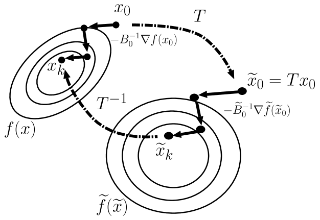
Figure 3: The coordinate transformation between $x$ of the function $f$ and $\widetilde{x}$ of the function $\widetilde{f}$ is depicted. The initial point $x_{0}$ is transformed to $\widetilde{x}_{0}=Tx_{0}$ and the search direction at $x_{0}$ is also transformed to $-\widetilde{B}_{0}^{-1}\nabla\widetilde{f}(\widetilde{x}_{0})$. The quasi-Newton method is applied to both $f(x)$ and $\widetilde{f}(\widetilde{x})$, and then the points $x_{k}$ and $\widetilde{x}_{k}$ are obtained in each coordinate system. If the equality $T^{-1}\widetilde{x}_{k}=x_{k}$ holds, the optimization algorithm is invariant under the transformation with $T$.

We consider the condition of $T$ such that the equality

$$T^{\top}\widetilde{B}_{k+1}T=B_{k+1},$$

holds, when $\widetilde{x}_{k}=Tx_{k}$ and $\widetilde{B}_{k}=(T^{\top})^{-1}B_{k}T^{-1}$ are satisfied. For such $T$, the equality $\widetilde{x}_{k+1}=Tx_{k+1}$ recursively holds. This implies that the point sequence obtained by the $V$-BFGS method is invariant under the affine transformation (22). In the optimization of $\widetilde{f}(\widetilde{x})$ by the $V$-BFGS method, the matrix $\widetilde{B}_{k}$ is updated to $\widetilde{B}_{k+1}$ such that

$$\widetilde{B}_{k+1} =\frac{\nu(\det{\widetilde{B}_{k+1}})}{\nu(\det{\widetilde{B}_{k}})}B^{BFGS}[\widetilde{B}_{k};\widetilde{s}_{k},\widetilde{y}_{k}]+\bigg{(}1-\frac{\nu(\det{\widetilde{B}_{k+1}})}{\nu(\det{\widetilde{B}_{k}})}\bigg{)}\frac{\widetilde{y}_{k}\widetilde{y}_{k}^{\top}}{\widetilde{s}_{k}^{\top}\widetilde{y}_{k}}.$$

Some calculation yields that

$$T^{\top}\widetilde{B}_{k+1}T =\frac{\nu(\det{\widetilde{B}_{k+1}})}{\nu(\det{\widetilde{B}_{k}})}B^{BFGS}[B_{k};s_{k},y_{k}]+\bigg{(}1-\frac{\nu(\det{\widetilde{B}_{k+1}})}{\nu(\det{\widetilde{B}_{k}})}\bigg{)}\frac{y_{k}y_{k}^{\top}}{s_{k}^{\top}y_{k}}.$$ (24)

The following theorem provides a sufficient condition on $T$ such that $T^{\top}\widetilde{B}_{k+1}T=B_{k+1}$ holds.

Theorem 5.

Suppose that $T\in\mathrm{SL}(n)$, that is, $\det(T)=1$. Then the equality $T^{\top}\widetilde{B}_{k+1}T=B_{k+1}$ holds for any $V$-BFGS update formula.

Proof.

Due to the assumption $\det(T)=1$, we have $\det(B_{k})=\det(\widetilde{B}_{k})$. Then Eq.(24) is equivalent with

$$T^{\top}\widetilde{B}_{k+1}T =\frac{\nu(\det{\widetilde{B}_{k+1}})}{\nu(\det{B_{k}})}B^{BFGS}[B_{k};s_{k},y_{k}]+\bigg{(}1-\frac{\nu(\det{\widetilde{B}_{k+1}})}{\nu(\det{B_{k}})}\bigg{)}\frac{y_{k}y_{k}^{\top}}{s_{k}^{\top}y_{k}}.$$

Hence, the determinant of $T^{\top}\widetilde{B}_{k+1}T$ yields the equality

$$\frac{\det(\widetilde{B}_{k+1})}{\nu(\det{\widetilde{B}_{k+1}})^{n-1}} =\frac{\det\big{(}B^{BFGS}[B_{k};s_{k},y_{k}]\big{)}}{\nu(\det{B_{k}})^{n-1}},$$

where $\det(T^{\top}\widetilde{B}_{k+1}T)=\det{\widetilde{B}_{k+1}}$ is used. On the other hand, the matrix $B_{k+1}$ defined by the $V$-BFGS update formula (19) also satisfies,

$$\frac{\det(B_{k+1})}{\nu(\det{B_{k+1}})^{n-1}} =\frac{\det\big{(}B^{BFGS}[B_{k};s_{k},y_{k}]\big{)}}{\nu(\det{B_{k}})^{n-1}},$$

As shown in the proof of Theorem 4, the function $z/\nu(z)^{n-1}$ is one to one mapping, and thus we have $\det{\widetilde{B}_{k+1}}=\det{B_{k+1}}$. Therefore, the equality $T^{\top}\widetilde{B}_{k+1}T=B_{k+1}$ holds. $\Box$

Next, we study the variable change with $T\in\mathrm{GL}(n)$. Below we assume $\nu(1)=1$ without loss of generality. Let us define

$$b_{k}=\det{B_{k}},\quad b_{k+1}=\det{B_{k+1}},\quad\widetilde{b}_{k+1}=\det{\widetilde{B}_{k+1}},\quad t=\det{T}$$

and

$$a=\frac{\det{B^{BFGS}[B_{k};s_{k},y_{k}]}}{\nu(\det{B_{k}})^{n-1}}.$$

In the $V$-BFGS update formula, the determinant of $B_{k+1}$ leads the equality

$$b_{k+1}=a\cdot\nu(b_{k+1})^{n-1}.$$ (25)

The matrix $\widetilde{B}_{k+1}$ satisfies the update formula (24), thus the determinant of both sides yields the equality

$$\widetilde{b}_{k+1}\,t^{2}=a\cdot\left(\frac{\nu(\widetilde{b}_{k+1})\nu(b_{k})}{\nu(b_{k}t^{-2})}\right)^{n-1}.$$ (26)

When $T^{\top}\widetilde{B}_{k+1}T=B_{k+1}$ holds, Eq.(26) is represented as

$$b_{k+1}=a\cdot\left(\frac{\nu(b_{k+1}t^{-2})\nu(b_{k})}{\nu(b_{k}t^{-2})}\right)^{n-1}.$$ (27)

We consider the function $\nu$ which satisfies (25) and (27) simultaneously. For a positive number $a>0$, let $b_{a}$ be the unique solution of the equation of $b$,

$$b=a\cdot\nu(b)^{n-1},\qquad b>0,$$

and $E_{\nu}=\{b_{a}\in\mathbb{R}~{}|~{}a>0\}$ be the set of all possible solutions of the above equation. Note that $1\in E_{\nu}$ holds for any $\nu$ since $1=1\cdot\nu(1)^{n-1}$ holds.

Theorem 6.

Let $\nu(z)>0$ be a differentiable function on $\mathbb{R}_{+}$. Suppose that there exists an open subset $E\subset\mathbb{R}$ satisfying $1\in E\subset E_{\nu}$. For the Hessian approximation by the $V$-BFGS method, suppose that the equality $\widetilde{B}_{k+1}=(T^{\top})^{-1}B_{k+1}T^{-1}$ holds for all $T\in\mathrm{GL}(n)$, all $B_{k}\in\mathrm{PD}(n)$ and all $s_{k},y_{k}\in\mathbb{R}^{n}$ satisfying $s_{k}^{\top}y_{k}>0$. Then the function $\nu$ is equal to $\nu(z)=z^{\gamma}$ with some $\gamma\in\mathbb{R}$.

Note that $E_{\nu}=\mathbb{R}_{+}$ holds for $\nu(z)=z^{\gamma}$ unless $\gamma=1/(n-1)$.

Proof.

Under the assumption, the equations (25) and (27) share the same solution $b_{k+1}$ for any $a>0,\,b_{k}>0$ and $t\neq 0$. Let $b_{k}=1,\,x=t^{-2}>0$. For any positive $a$ and $x$, equations (25) and (27) lead to

$$b_{a}=a\cdot\nu(b_{a})^{n-1}\ \ \text{and}\ \ b_{a}=a\cdot\nu(b_{a}x)^{n-1}\left(\frac{\nu(1)}{\nu(x)}\right)^{n-1}=a\cdot\frac{\nu(b_{a}x)^{n-1}}{\nu(x)^{n-1}}$$

for $b_{a}\in E_{\nu}$. Hence we obtain

$$\nu(b_{a}x)=\nu(b_{a})\nu(x),\ \ a>0,\ x>0\ \Longleftrightarrow\ \nu(bx)=\nu(b)\nu(x),\ \ b\in E_{\nu},\ x>0.$$ (28)

The assumption on $E_{\nu}$ guarantees that $1+\varepsilon\in E_{\nu}$ holds for any infinitesimal $\varepsilon$. Thus Eq.(28) leads the following expression,

$$\frac{\nu(x(1+\varepsilon))-\nu(x)}{x\varepsilon}=\frac{\nu(x)}{x}\cdot\frac{\nu(1+\varepsilon)-\nu(1)}{\varepsilon}.$$

Taking the limit $\varepsilon\rightarrow 0$, we obtain the differential equation,

$$\nu^{\prime}(x)=\nu^{\prime}(1)\frac{\nu(x)}{x},\qquad\nu(1)=1,$$

and the solution is given as $\nu(x)=x^{\nu^{\prime}(1)}$. $\Box$

As shown in Example 2, the function $\nu(z)=z^{\gamma}$ is derived from the power potential $V(z)=(1-z^{\gamma})/\gamma$. In robust statistics, the power potential has been applied in wide-rage of data analysis [4, 21].

Remark 1.

Ohara and Eguchi [26] have studied the differential geometrical structure over $\mathrm{PD}(n)$ induced by the $V$-Bregman divergence. They pointed out that the geometrical structure is invariant under $\mathrm{SL}(n)$ group action. Furthermore, they have showed that for the power potential $V(z)=(1-z^{\gamma})/\gamma$, the $\theta_{V}$- ($\eta$-) projection onto $\eta$- ($\theta_{V}$-) autoparallel submanifold is invariant under $\mathrm{GL}(n)$ group action. It turns out that only the orthogonality is kept unchanged under the group action. The other geometrical features such as angle between two tangent vectors are not preserved in general. Theorem 6 indicates that the invariance of the geometrical structure on $\mathrm{PD}(n)$ is inherited to the invariance of point sequences of quasi-Newton methods under the affine transformation.

In summary, we obtain the following results. Suppose that $\widetilde{x}_{0}=Tx_{0},\,\widetilde{B}_{0}=(T^{\top})^{-1}B_{0}T^{-1}$ holds. Let $\{x_{k}\}$ and $\{\widetilde{x}_{k}\}$ be point sequences generated by the $V$-BFGS method for the functions $f(x)$ and $\widetilde{f}(\widetilde{x})$, respectively. Suppose that the line search with the same stopping rule is used for the step length. Then, for any $T\in\mathrm{SL}(n)$ the equality $\widetilde{x}_{k}=Tx_{k}$ holds for all $k\geq 1$. Moreover the equality $\widetilde{x}_{k}=Tx_{k},\,k\geq 1$ holds for any $T\in\mathrm{GL}(n)$ if and only if the function $V(z)$ is the power potential.

5 Geometry of Sparse quasi-Newton updates

Sparse quasi-Newton method exploits the sparsity of Hessian matrix in order to reduce the computation cost [32]. The sparsity pattern of the Hessian matrix at a point $x\in\mathbb{R}^{n}$ is represented by an index set $F$ satisfying

$$\{(i,j)~{}|~{}(\nabla^{2}f(x))_{ij}\neq 0\}\subset F.$$

When the number of entries in $F$ is small, the matrix $\nabla^{2}f(x)$ is referred to as sparse matrix. We assume that $(j,i)\in F$ holds for $(i,j)\in F$ and that $(i,i)\in F$ for all $i=1,\ldots,n$. Given a sparsity pattern $F$, the set of sparse matrix is defined by

$$\mathcal{S}=\{P\in\mathrm{PD}(n)~{}|~{}P_{ij}=0\ \text{for}\ (i,j)\not\in F\}.$$

Clearly the submanifold $\mathcal{S}$ is $\eta$-autoparallel in $\mathrm{PD}(n)$.

Yamashita [32] has proposed a sparse quasi-Newton method. In this section we show an extension of sparse quasi-Newton method and illustrate a geometrical structure of the update formula. First, we briefly introduce the sparse quasi-Newton method proposed by Yamashita [32]. Suppose $H_{k}$ be an approximate inverse Hessian matrix at the $k$-th step of the sparse quasi-Newton method. Let $H_{k}^{\mathrm{QN}}$ be the updated matrix of $H_{k}$ by the existing quasi-Newton methods such as the BFGS or the DFP method for the approximate inverse Hessian matrix. In the computation of $H_{k}^{\mathrm{QN}}$, we need only the elements $(H_{k}^{\mathrm{QN}})_{ij}$ for $(i,j)\in F$, and thus efficient computation will be possible even if the size of the matrix is large. Then, compute the sparse matrix $H_{k+1}\in\mathcal{S}$ satisfying the constraint $(H_{k+1})_{ij}=(H_{k}^{\mathrm{QN}})_{ij}$ for all $(i,j)\in{F}$. The calculation of $H_{k+1}$ from $H_{k}^{\mathrm{QN}}$ is regarded as the $\theta_{V}$-projection with respect to the KL-divergence. The sparse clique-factorization technique [13, 15] is available for the practical computation of the projection. See [32] for details.

For the computation of both $H^{\mathrm{QN}}_{k+1}$ and $H_{k+1}$ in the sparse quasi-Newton method, we can use Bregman divergence instead of the KL-divergence. Figure 4 shows an extended sparse quasi-Newton method for the approximate Hessian matrix $B_{k}$. Figure 5 illustrates the geometrical interpretation of the extended sparse quasi-Newton updates.

We have some choices in the algorithm of Figure 4: (i) the Bregman divergence in Step 2, (ii) projection in Step 3, and (iii) the number of $T$. In the sparse quasi-Newton updates presented by Yamashita [32] , the number of iteration is set to $T=1$; in Step 2, the standard BFGS/DFP method for the approximate inverse Hessian is used; in Step 3 the $\theta_{V}$-projection defined from the KL-divergence is computed. Moreover, the superlinear convergence has been proved, see [32] for details. In the following, we present the geometrical interpretation of the sparse quasi-Newton method. Then we show a computation algorithm for the update formula derived from the $V$-Bregman divergence.

Extended sparse quasi-Newton update algorithm: the Hessian approximation $B_{k}$ at the $k$-th step of quasi-Newton method is updated to a sparse matrix $B_{k+1}$. Suppose that the Bregman divergence is defined from the potential function $\varphi$, and let $\mathcal{S}$ be the set of sparse matrix defined by a fixed index set $F$. Initialization: Let $T$ be an positive integer, and $B^{(0)}:=B_{k}$. Repeat: $t=1,2,\ldots,T$. 1. Compute the partial matrix $\bar{B}^{(t-1)}_{ij}$ for $(i,j)\in F$ from $B^{(t-1)}$ by using the extended quasi-Newton method such as (16) or (17). 2. Compute the sparse matrix $B^{(t)}\in\mathcal{S}$ which is the $\theta_{\varphi}$-projection of $\bar{B}^{(t-1)}$ onto $\mathcal{S}$. Output: The updated approximate Hessian matrix $B_{k+1}$ is given as $B^{(T)}\in\mathcal{S}$.

Figure 4: An extension of sparse quasi-Newton method is presented. The approximate Hessian $B_{k}$ is updated to $B_{k+1}$ by exploiting the update formula with Bregman divergences.

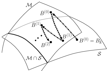
Figure 5: Geometrical illustration of the extended sparse quasi-Newton update algorithm.

5.1 Geometry of Sparse quasi-Newton update

We consider the sparse quasi-Newton update formula from the geometrical viewpoint. Remember that $\mathcal{M}$ is the set of matrices satisfying the secant condition

$$\mathcal{M}=\{B\in\mathrm{PD}(n)~{}|~{}Bs_{k}=y_{k}\}.$$

Below we consider two kinds of update formulae:

Algorithm 1:

In the algorithm in Figure 4, the matrix $\bar{B}^{(t)}$ is defined as the $\eta$-projection of $B^{(t)}$ onto $\mathcal{M}$, that is, $\bar{B}^{(t)}$ is equal to $B^{DFP}[B^{(t)};s_{k},t_{k}]$. Then $B^{(t+1)}$ is defined as the $\theta_{\varphi}$-projection of $\bar{B}^{(t)}$ onto $\mathcal{S}$.

Algorithm 2:

In the algorithm in Figure 4, the matrix $\bar{B}^{(t)}$ is the $\theta_{\varphi}$-projection of $B^{(t)}$ onto $\mathcal{M}$, that is, $\bar{B}^{(t)}$ is given as the optimal solution of (16). Then $B^{(t+1)}$ is defined as the $\theta_{\varphi}$-projection of $\bar{B}^{(t)}$ onto $\mathcal{S}$.

The difference between Algorithm 1 and Algorithm 2 is the projection onto $\mathcal{M}$ to obtain $\bar{B}^{(t)}$. Below we show the theoretical properties for each algorithm.

In Algorithm 1, we consider how the Bregman divergence $D_{\varphi}(B^{(t)},\bar{B}^{(t)})$ is updated. Let $B^{(0)}=B_{k}\in\mathcal{S}$ and suppose that the $\theta_{\varphi}$-projection onto $\mathcal{S}$ exists. Then, the extended Pythagorean theorem in Section 2.3 leads that

$$D_{\varphi}(B^{(t)},\bar{B}^{(t)}) =D_{\varphi}(B^{(t)},B^{(t+1)})+D_{\varphi}(B^{(t+1)},\bar{B}^{(t)})$$

$$=D_{\varphi}(B^{(t)},B^{(t+1)})+D_{\varphi}(B^{(t+1)},\bar{B}^{(t+1)})+D_{\varphi}(\bar{B}^{(t+1)},\bar{B}^{(t)})$$

$$\geq D_{\varphi}(B^{(t+1)},\bar{B}^{(t+1)})$$

and hence we have

$$D_{\varphi}(B^{(0)},\bar{B}^{(0)})\geq D_{\varphi}(B^{(1)},\bar{B}^{(1)})\geq\cdots\geq D_{\varphi}(B^{(T)},\bar{B}^{(T)}).$$

This indicates that under a mild assumption the Bregman divergence $D_{\varphi}(B^{(t)},\bar{B}^{(t)})$ will converge to zero and that $B^{(t)}\in\mathcal{S}$ will also converge to a matrix in $\mathcal{M}\cap\mathcal{S}$. A condition on the convergence has been investigated by Bauschke, et al. [5]. This update algorithm is similar to the so-called em-algorithm [1, 8] which is a popular algorithm in statistics and machine learning. In the em-algorithm, the $\eta$-projection and the $\theta_{V}$-projection with $V(z)=-\log z$ is repeated in the probability space. Then, the maximum likelihood estimator under the partial observation is computed. In the context of statistical estimation, usually the em-algorithm is conducted when $\mathcal{M}\cap\mathcal{S}=\emptyset$ holds. Under some assumption with $\mathcal{M}\cap\mathcal{S}=\emptyset$, the point sequences $(B^{(t)},\bar{B}^{(t)})\in\mathcal{S}\times\mathcal{M}$ converges to the pair of the closest point $(B^{\ast},\bar{B}^{\ast})\in\mathcal{S}\times\mathcal{M}$ such that $(B^{\ast},\bar{B}^{\ast})$ is the optimal solution of the optimization problem,

$$\min_{(B,\bar{B})\in\mathcal{S}\times\mathcal{M}}D_{\varphi}(B,\bar{B}),$$

see [20] for details. We believe that to provide a simple characterization about the convergence point $(B^{\ast},\bar{B}^{\ast})$ under the condition $\mathcal{M}\cap\mathcal{S}\neq\emptyset$ is an open problem.

Next, we investigate Algorithm 2. Likewise we suppose $B_{k}=B^{(0)}\in\mathcal{S}$. Note that $\mathcal{M}\cap\mathcal{S}$ is $\eta$-autoparallel. Let $B^{\star}$ be the $\theta_{\varphi}$-projection of $B_{k}=B^{(0)}$ onto the intersection $\mathcal{M}\cap\mathcal{S}$. Then the extended Pythagorean theorem leads that

$$D_{\varphi}(B^{\star},B^{(t)}) =D_{\varphi}(B^{\star},\bar{B}^{(t)})+D_{\varphi}(\bar{B}^{(t)},B^{(t)})$$

$$=D_{\varphi}(B^{\star},B^{(t+1)})+D_{\varphi}(B^{(t+1)},\bar{B}^{(t)})+D_{\varphi}(\bar{B}^{(t)},B^{(t)})$$

$$\geq D_{\varphi}(B^{\star},B^{(t+1)})$$

and hence we have

$$D_{\varphi}(B^{\star},B^{(0)})\geq D_{\varphi}(B^{\star},B^{(1)})\geq\cdots\geq D_{\varphi}(B^{\star},B^{(T)}).$$

Suppose that $B^{(T)}$ converges to $B^{(\infty)}\in\mathcal{M}\cap\mathcal{S}$ when $T$ tends to infinity, then the equality $B^{(\infty)}=B^{\star}$ holds as shown below. From the definition of $B^{\star}$ and the extended Pythagorean theorem, we have

$$D_{\varphi}(B^{(\infty)},B^{(T)})=D_{\varphi}(B^{(\infty)},B^{*})+D_{\varphi}(B^{*},B^{(T)}).$$

Due to the continuity of the Bregman divergence, for $T\rightarrow\infty$ we have

$$0=D_{\varphi}(B^{(\infty)},B^{(\infty)})=D_{\varphi}(B^{(\infty)},B^{*})+D_{\varphi}(B^{*},B^{(\infty)}),$$

and hence $B^{(\infty)}=B^{\star}$ holds. As the result we have $\lim_{T\rightarrow\infty}B^{(T)}=B^{\star}$. Figure 6 shows the geometrical illustration of the Algorithm 2. Applying Theorem 8.1 of Bauschke and Borwein [6], we see that the convergence of $B^{(T)}$ to the point $B^{\star}$ is guaranteed under the Bregman divergence associated with power potential with $\gamma\leq 0$. The iterative update procedure is closely related to the boosting algorithm [12, 22] in which the iterative Bregman projection is exploited to compute the estimator for classification problems.

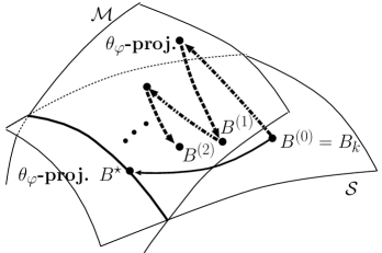
Figure 6: Geometrical interpretation of Algorithm 2. The sparse matrix $B^{(t)}$ will converge to $B^{\star}$ which is the $\theta_{\varphi}$ projection of $B^{(0)}=B_{k}\in\mathcal{S}$.

As argued above, it is not guaranteed that $B^{(t)}$ in Algorithm 1 converges to $B^{\star}$, which is the $\theta_{\varphi}$-projection of $B_{k}=B^{(0)}$ onto $\mathcal{M}\cap\mathcal{S}$. On the other hand the sequence $B^{(t)}$ in Algorithm 2 converges to $B^{\star}$ under mild assumption. From the viewpoint of the least-change principle, the sparse quasi-Newton method with Algorithm 2 will be preferable. Fletcher [11] has proposed the sparse update formula using $B^{\star}$. The update formula using the matrix $B^{\star}$ requires the sparsity and the secant condition simultaneously, and hence, the approximate Hessian can be ill-posed when $(s_{k})_{i}=0$ for some $i$ [31].

5.2 Computation of Projections

We consider the computation of the extended sparse quasi-Newton updates. In Algorithm 1 and 2 above, we need to compute the $\theta_{\varphi}$-projection of a matrix $B$ onto the $\eta$-autoparallel submanifold $\mathcal{S}$ consisting of sparse positive definite matrices. Generally the $\theta_{\varphi}$-projection does not have the explicit expression. Here, we study only the $\theta_{V}$-projection based on the $V$-Bregman divergence.

According to Yamashita [32], we briefly introduce the computation of the projection onto $\mathcal{S}$, when the geometrical structure is induced from the KL-divergence. For a given matrix $\bar{B}^{(t)}\in\mathcal{M}$, the projection onto $\mathcal{S}$, denoted as $B^{(t+1)}$, is obtained as the optimal solution of

$$\min_{B\in\mathcal{\mathrm{PD}}(n)}\mathrm{KL}(B,\bar{B}^{(t)}),\qquad\text{\rm s.\,t.\ }B\in\mathcal{S}.$$

Some calculation yields that $B^{(t+1)}$ is also the optimal solution of

$$\max_{B\in\mathcal{\mathrm{PD}}(n)}\det{B^{-1}},\qquad\text{\rm s.\,t.\ }(B^{-1})_{ij}=(H^{(t)})_{ij}\ \ (i,j)\in F.$$

Let $\bar{F}$ be $\bar{F}=F\backslash\{(i,i)~{}|~{}i=1,\ldots,n\}$. If the graph $G=(\{1,\ldots,n\},\bar{F})$ is chordal, the existence of the optimal solution is guaranteed [32, 13, 15]. The inverse of the optimal solution, $(B^{(t+1)})^{-1}$, is represented by using the sparse clique-factorization formula [13, 32], and then the updated inverse Hessian matrix is obtained. The sparse clique-factorization formula of $(B^{(t+1)})^{-1}$ is represented by

$$(B^{(t+1)})^{-1}=L_{1}^{\top}L_{2}^{\top}\cdots L_{\ell-1}^{\top}DL_{\ell-1}\cdots L_{2}L_{1}$$

in which $L_{r}\;(r=1,\ldots,\ell-1)$ are lower triangular matrices, and $D$ is a positive definite block-diagonal matrix consisting of $\ell$ diagonal blocks. The number of $\ell$ is determined by the the number of maximal cliques of the graph $G=(\{1,\ldots,n\},\bar{F})$, and all elements of $L_{r}\;(r=1,\ldots,\ell-1)$ and $D$ are explicitly computed from $(H^{(t)})_{ij},\,(i,j)\in F$. We generalize the above argument to the projection with the $V$-Bregman divergence.

Theorem 7.

Let $\bar{F}$ be $\bar{F}=F\backslash\{(i,i)~{}|~{}i=1,\ldots,n\}$, and suppose that the undirected graph $(\{1,\ldots,n\},\bar{F})$ is chordal. Let $\bar{B}^{(t)}\in\mathcal{M}$. Then there exists the $\theta_{V}$-projection of $\bar{B}^{(t)}$ onto $\mathcal{S}$, and the projection is the optimal solution of the following problem,

$$\begin{array}[]{l}\displaystyle\min_{B\in\mathrm{PD}(n)}\ \det(B),\quad\text{\rm subject to }\ (\theta_{V}(B))_{ij}=(\theta_{V}(\bar{B}^{(t)}))_{ij},\ (i,j)\in F.\end{array}$$ (30)

Proof.

Remember that $\theta_{V}(P)$ is defined as $\theta_{V}(P)=-\nu(\det{P})P^{-1}$ which is a negative definite matrix. It is easy to see that the mapping $-\theta_{V}(P)$ is bijection on $\mathrm{PD}(n)$. Hence, the assumption on the graph $(\{1,\ldots,n\},\bar{F})$ guarantees that the problem

$$\max_{B\in\mathrm{PD}(n)}\det(-\theta_{V}(B)),\qquad(\theta_{V}(B))_{ij}=(\theta_{V}(\bar{B}^{(t)}))_{ij}\;\;\text{for all}\;\;(i,j)\in F$$ (31)

has the unique optimal solution $B^{*}$, and the optimal solution satisfies $(-\theta_{V}(B^{*}))^{-1}\in\mathcal{S}$, as shown in [15, 13, 32]. In terms of the objective function, we see that

$$\det(-\theta_{V}(B))=\det(\nu(\det{B})B^{-1})=\frac{\nu(\det{B})^{n}}{\det{B}}.$$

The function $\nu(z)^{n}/z$ is strictly monotone decreasing for $z>0$. Indeed,

$$\frac{d}{dz}\log\frac{\nu(z)^{n}}{z}=\frac{n}{z}\bigg{(}\beta(z)-\frac{1}{n}\bigg{)}<0$$

holds. Thus, the optimal solution of (31) is identical to that of (30). We find that $B^{*}\in\mathcal{S}$ holds, since $(-\theta_{V}(B^{*}))^{-1}=\nu(\det{B^{*}})^{-1}B^{*}\in\mathcal{S}$ holds. For any $B\in\mathcal{S}$, we have

$$D_{V}(B,\bar{B}^{(t)})-D_{V}(B,B^{*})-D_{V}(B^{*},\bar{B}^{(t)}) =\sum_{i,j}(\theta_{V}(\bar{B}^{(t)})-\theta_{V}(B^{*}))_{ij}(B^{*}-B)_{ij}$$

$$=\sum_{(i,j)\not\in F}(\theta_{V}(\bar{B}^{(t)})-\theta_{V}(B^{*}))_{ij}(B^{*}-B)_{ij}$$

$$=0.$$

The second and third equalities follows $(\theta_{V}(\bar{B}^{(t)})-\theta_{V}(B^{*}))_{ij}=0$ for $(i,j)\in F$ and $(B^{*}-B)_{ij}=0$ for $(i,j)\not\in F$, respectively. Therefore, $B^{*}$ is identical to the $\theta_{V}$-projection of $\bar{B}_{t}$ onto $\mathcal{S}$. $\Box$

We present a practical method of computing the projection of $\bar{B}^{(t)}$ onto $\mathcal{S}$. Let $B^{(t)}$ and $\bar{B}^{(t)}$ for $t=0,1,2,\ldots$ be matrices generated by the extended sparse quasi-Newton update with Algorithm 2. We show a method of computing $H^{(t)}=(B^{(t)})^{-1}$ and $\bar{H}^{(t)}=(\bar{B}^{(t)})^{-1}$. Suppose we have $H^{(t)}$, then $\bar{H}^{(t)}$ is obtained by solving the problem

$$\min_{H\in\mathrm{PD}(n)}D_{V}(H^{-1},(H^{(t)})^{-1}),\qquad Hy_{k}=s_{k}.$$

In the similar way of the proof of Theorem 4, the optimal solution $\bar{H}^{(t)}$ satisfies

$$\bar{H}^{(t)}=\frac{\nu(\det({\bar{H}^{(t)}})^{-1})}{\nu(\det({H^{(t)}})^{-1})}B^{\mathrm{DFP}}[H^{(t)};y_{k},s_{k}]+\bigg{(}1-\frac{\nu(\det({\bar{H}^{(t)}})^{-1})}{\nu(\det({H^{(t)}})^{-1})}\bigg{)}\frac{s_{k}s_{k}^{\top}}{s_{k}^{\top}y_{k}}.$$

We need only the elements $(\bar{H}^{(t)})_{ij}$ for $(i,j)\in F$ and the determinant $\det(\bar{H}^{(t)})$. If we have the Choleskey factorization or the sparse clique-factorization formula of $H^{(t)}$, we can obtain these values by simple computation. Then, the matrix $H^{(t+1)}$ is given as the optimal solution of

$$\min_{H\in\mathrm{PD}(n)}D_{V}(H^{-1},(\bar{H}^{(t)})^{-1}),\qquad H^{-1}\in\mathcal{S}.$$

As shown in the proof of Theorem 7, $H^{(t+1)}$ is also the optimal solution of

$$\max_{H\in\mathrm{PD}(n)}\det(-\theta_{V}(H^{-1})),\qquad\theta_{V}(H^{-1})_{ij}=\theta_{V}((\bar{H}^{(t)})^{-1})_{ij}\;\;\text{for all}\;\;(i,j)\in F$$

Let $X=-\theta_{V}((H^{(t+1)})^{-1})=\nu(\det(H^{(t+1)})^{-1})H^{(t+1)}$, then the sparse clique-factorization formula provides the factorized expression of $X$ based on the information of $\nu(\det(\bar{H}^{(t)})^{-1})\bar{H}^{(t)}_{ij},\,(i,j)\in F$. The determinant of $X$ is easily computed by the sparse clique-factorization formula. Then, we solve the the following equation,

$$\det{X}=\frac{\nu(z)^{n}}{z},\quad z>0.$$

The Newton method is available to find the unique solution $z^{*}$ efficiently. Using the solution $z^{*}$, the matrix $H^{(t+1)}$ is represented

$$H^{(t+1)}=\frac{1}{\nu(z^{*})}X.$$

The matrix $H^{(t+1)}$ also has the expression of the sparse clique-factorization formula, and thus, it is available to the sequel computation.

6 Concluding Remarks

Along the line of the research stared by Fletcher [10], we considered the quasi-Newton update formula based on the Bregman divergences, and presented a geometrical interpretation of the Hessian update formulae. We studied the invariance property of the update formulae. The sparse quasi-Newton methods were also considered based on the information geometry. We show that the information geometry is useful tool not only to better understand the quasi-Newton methods but also to design new update formulae.

As pointed out in Section 3, the self-scaling quasi-Newton method with the popular scaling parameter is out of the formulae derived from the Bregman divergence. Nocedal and Yuan proved that the self-scaling quasi-Newton method with the popular scaling parameter has some drawbacks [24]. An interesting future work is to pursue the relation between the numerical properties and the geometrical structure behind the optimization algorithms. In the study of the interior point methods, it has been made clear that geometrical viewpoint is useful [28]. The geometrical viewpoint will become important to investigate algorithms for numerical computation.

7 Acknowledgements

The authors are grateful to Dr. Nobuo Yamashita of Kyoto university for helpful comments. T. Kanamori was partially supported by Grant-in-Aid for Young Scientists (20700251).

Appendix A Proof of Theorems 4

We prove the following lemma which is useful to show the existence of the optimal solution.

Lemma 8.

Let $V$ be a potential and $\nu=\nu_{V}$. For any $C>0$ the equation

$$C\nu(z)^{n-1}=z,\quad z>0$$ (32)

has the unique solution.

Proof.

We define the function $\zeta(z)$ by $\zeta(z)=\log z-(n-1)\log\nu(z)$, then, the (32) is equivalent to the equation

$$\log C=\zeta(z),\quad z>0.$$ (33)

Since the potential function satisfies $\lim_{z\rightarrow+0}z/\nu(z)^{n-1}=0$ from the definition, we have $\lim_{z\rightarrow+0}\zeta(z)=-\infty$. In terms of the derivative of $\zeta(z)$, we have the following inequality

$$\frac{d}{dz}\zeta(z)=\frac{1}{z}-(n-1)\frac{\beta(z)}{z}>\frac{1}{zn}>0.$$

Thus, $\zeta(z)$ is an increasing function on $\mathbb{R}_{+}$. Moreover we have

$$\zeta(z)\geq\zeta(1)+\int_{1}^{z}\frac{1}{zn}dz=\zeta(1)+\frac{\log z}{n}.$$

The above inequality implies that $\lim_{z\rightarrow\infty}\zeta(z)=\infty$. Since $\zeta(z)$ is continuous, the equation (33) has the unique solution. $\Box$

Proof of Theorem 4.

First, we show the existence of the matrix $B_{k+1}$ satisfying (19). Lemma 8 now shows that there exists a solution $z^{*}>0$ for the equation

$$\frac{\det(B^{BFGS}[B_{k};s_{k},y_{k}])}{\nu(\det{B_{k}})^{n-1}}\cdot\nu(z)^{n-1}=z,\quad z>0.$$

By using the solution $z^{*}$, we define the matrix $\bar{B}$ such that

$$\bar{B}=\frac{\nu(z^{*})}{\nu(\det{B_{k}})}B^{BFGS}[B_{k};s_{k},y_{k}]+\big{(}1-\frac{\nu(z^{*})}{\nu(\det{B_{k}})}\big{)}\frac{y_{k}y_{k}^{\top}}{s_{k}^{\top}y_{k}},$$

then the determinant of $\bar{B}$ satisfies

$$\det{\bar{B}}=\frac{\det(B^{BFGS}[B_{k}])}{\nu(\det{B_{k}})^{n-1}}\cdot\nu(z^{*})^{n-1}=z^{*},$$

in which the first equality comes from the formula $\det(A+vu^{\top})=\det(A)(1+u^{\top}A^{-1}v)$ and the second one follows the definition of $z^{*}$. Hence there exists $B_{k+1}\in\mathrm{PD}(n)$ satisfying (19).

Next, we show that the matrix $B_{k+1}$ in (19) satisfies the optimality condition of (18). According to Güler, et al. [16], the normal vector for the affine subspace

$$\mathcal{M}=\{B\in\mathrm{PD}(n)~{}|~{}Bs_{k}=y_{k}\}$$

is characterized by the form of

$$s_{k}\lambda^{\top}+\lambda s_{k}^{\top}\in\mathrm{Sym}(n),\qquad\lambda\in\mathbb{R}^{n}.$$ (34)

Suppose $B^{\prime}\in\mathrm{PD}(n)$ be an optimal solution of (18), then $B^{\prime}$ satisfies the optimality condition that there exists a vector $\lambda\in\mathbb{R}^{n}$ such that

$$\phantom{\Longleftrightarrow}\nabla_{B}D_{V}(B,B_{k})\big{|}_{B=B^{\prime}}=s_{k}\lambda^{\top}+\lambda s_{k}^{\top}$$

$$\Longleftrightarrow\ -\nu(\det(B^{\prime}))(B^{\prime})^{-1}+\nu(\det(B_{k}))B_{k}^{-1}=s_{k}\lambda^{\top}+\lambda s_{k}^{\top},$$

where $\nabla_{B}D_{V}(B,B_{k})$ denotes the gradient of $D_{V}(B,B_{k})$ with respect to the variable $B$. Also, the optimal solution $B^{\prime}$ should satisfy the constraint $B^{\prime}s_{k}=y_{k}$. On the other hand, the matrix $B_{k+1}$ defined by (19) satisfies

$$B_{k+1}^{-1} =\frac{\nu(\det{B_{k}})}{\nu(\det{B_{k+1}})}(B^{BFGS}[B_{k};s_{k},y_{k}])^{-1}+\bigg{(}1-\frac{\nu(\det{B_{k}})}{\nu(\det{B_{k+1}})}\bigg{)}\frac{s_{k}s_{k}^{\top}}{s_{k}^{\top}y_{k}}$$

$$=\frac{\nu(\det{B_{k}})}{\nu(\det{B_{k+1}})}B^{DFP}[B_{k}^{-1};y_{k},s_{k}]+\bigg{(}1-\frac{\nu(\det{B_{k}})}{\nu(\det{B_{k+1}})}\bigg{)}\frac{s_{k}s_{k}^{\top}}{s_{k}^{\top}y_{k}}$$

$$\Longleftrightarrow \left\{\begin{array}[]{l}\displaystyle-\nu(\det{B_{k+1}})B_{k+1}^{-1}+\nu(\det{B_{k}})B_{k}^{-1}=s_{k}\lambda^{\top}+\lambda s_{k}^{\top},\vspace*{2mm}\\ \displaystyle\lambda=\frac{\nu(\det{B_{k}})}{s_{k}^{\top}y_{k}}B_{k}^{-1}y_{k}-\frac{\nu(\det{B_{k+1}})}{2s_{k}^{\top}y_{k}}s_{k}-\frac{\nu(\det{B_{k}})y_{k}^{\top}B_{k}^{-1}y_{k}}{2(s_{k}^{\top}y_{k})^{2}}s_{k}.\end{array}\right.$$

The conditions $s_{k}^{\top}y_{k}>0$ and $B_{k}\in\mathrm{PD}(n)$ guarantees the existence of the above vector $\lambda$. In addition, the direct computation yields that the constraint $B_{k+1}s_{k}=y_{k}$ is satisfied. Hence, $B_{k+1}$ satisfies the optimality condition. Since (18) is a strictly convex problem, $B_{k+1}$ is the unique optimal solution. $\Box$

References

• [1] S. Amari. Information geometry of the EM and em algorithms for neural networks. Neural Networks, 8(9):1379–1408, 1995.
• [2] S. Amari and H. Nagaoka. Methods of Information Geometry, volume 191 of Translations of Mathematical Monographs. Oxford University Press, 2000.
• [3] A. Banerjee, S. Merugu, I. Dhillon, and J. Ghosh. Clustering with Bregman divergences. Journal of Machine Learning Research, 6:1705–1749, 2005.
• [4] A. Basu, I. R. Harris, N. L. Hjort, and M. C. Jones. Robust and efficient estimation by minimising a density power divergence. Biometrika, 85(3):549–559, 1998.
• [5] H. H. Bauschke and P. L. Combettes. Iterating Bregman retractions. SIAM J. on Optimization, 13(4):1159–1173, 2002.
• [6] H.H. Bauschke and J.M. Borwein. Legendre functions and the method of random Bregman projections. Journal of Convex Analysis, 4(1):27–67, 1997.
• [7] L. M. Bregman. The relaxation method of finding the common point of convex sets and its application to the solution of problems in convex programming. USSR Computational Mathematics and Mathematical Physics, 7:200–217, 1967.
• [8] A. P. Dempster, N. M. Laird, and D. B. Rubin. Maximum likelihood from incomplete data via the em algorithm. Journal of the Royal Statistical Society, B, 39:1–38, 1977.
• [9] I. S. Dhillon and J. A. Tropp. Matrix nearness problems with Bregman divergences. SIAM J. Matrix Anal. Appl., 29(4):1120–1146, 2007.
• [10] R. Fletcher. A new variational result for quasi-Newton formulae. SIMA J. Optim., 1:18–21, 1991.
• [11] R. Fletcher. An optimal positive definite update for sparse hessian matrices. SIMA J. Optim., 5:192–218, 1995.
• [12] Y. Freund and R. E. Schapire. A decision-theoretic generalization of on-line learning and an application to boosting. Journal of Computer and System Sciences, 55(1):119–139, aug 1997.
• [13] M. Fukuda, M. Kojima, K. Murota, and K. Nakata. Exploiting sparsity in semidefinite programming via matrix completion I: General framework. SIAM J. on Optimization, 11(3):647–674, 2000.
• [14] P. E. Gill and W. Murray. Quasi-Newton methods for unconstrained optimization. J. Inst. Maths. Applns., 9:91–108, 1972.
• [15] R. Grone, C. R. Johnson, E. M. Sá, and H. Wolkowicz. Positive definite completions of partial hermitian matrices. Linear Algebra and its Applications, 58:109–124, 1984.
• [16] O. Güler, F. Gürtuna, and O. Shevchenko. Duality in quasi-Newton methods and new variational characterizations of the DFP and BFGS updates. Optimization Methods and Software, 24(1):45–62, 2009.
• [17] T. Kanamori and A. Ohara. A Bregman extension of quasi-Newton updates II: Convergence and robustness properties. submitted, 2010.
• [18] S. Kobayashi and K. Nomizu. Foundations of Differential Geometry. Wiley-Interscience, 1996.
• [19] S. Kullback and R. A. Leibler. On information and sufficiency. The Annals of Mathematical Statistics, 22(1):79–86, 1951.
• [20] G. J. McLachlan and T. Krishnam. The EM algorithm and extensions. Wiley, 2nd edition, 2008.
• [21] M. Minami and S. Eguchi. Robust blind source separation by beta-divergence. Neural Computation, 14(8):1859–1886, 2002.
• [22] N. Murata, T. Takenouchi, T. Kanamori, and S. Eguchi. Information geometry of $U$-Boost and Bregman divergence. Neural Computation, 16(7):1437–1481, 2004.
• [23] J. Nocedal and S. Wright. Numerical Optimization. Springer, 1999.
• [24] J. Nocedal and Y-X. Yuan. Analysis of a self-scaling quasi-Newton method. Math. Program., 61:19–37, 1993.
• [25] A. Ohara. Information geometric analysis of an interior point method for semidefinite programming. In O.E. Barndorff-Nielsen and E.B. Vedel Jensen, editors, Geometry in Present Day Science, pages 49–74. World Scientific, 1999.
• [26] A. Ohara and S. Eguchi. Geometry on positive definite matrices and v-potential function. Technical report, ISM Research Memo, 2005.
• [27] A. Ohara, N. Suda, and S. Amari. Dualistic differential geometry of positive definite matrices and its applications to related problems. Linear Algebra and Its Applications, 247:31–053, 1996.
• [28] A. Ohara and T. Tsuchiya. An information geometric approach to polynomial-time interior-point algorithms -complexity bound via curvature integral. Foundation of Computational Mathematics, 2010. submitted for publication.
• [29] S. S. Oren and D. G. Luenberger. Self-scaling variable metric (ssvm) algorithms, part i. criteria and sufficient conditions for scaling a class of algorithms. Management Science, 20:845–862, 1974.
• [30] R. T. Rockafellar. Convex Analysis. Princeton University Press, 1970.
• [31] D. C. Sorensen. Collinear scaling and sequential estimation in sparse optimization algorithm. Math. Program. Stud., 18:135–159, 1982.
• [32] N. Yamashita. Sparse quasi-Newton updates with positive definite matrix completion. Math. Program., 115(1):1–30, 2008.