Electronic Transport in Disordered Bilayer and Trilayer Graphene

Abstract

We present a detailed numerical study of the electronic transport properties of bilayer and trilayer graphene within a framework of single-electron tight-binding model. Various types of disorder are considered, such as resonant (hydrogen) impurities, vacancies, short- or long-range Gaussian random potentials, and Gaussian random nearest neighbor hopping. The algorithms are based on the numerical solution of the time-dependent Schrödinger equation and applied to calculate the density of states and conductivities (via the Kubo formula) of large samples containing millions of atoms. In the cases under consideration, far enough from the neutrality point, depending on the strength of disorders and the stacking sequence, a linear or sublinear electron-density dependent conductivity is found. The minimum conductivity $\sigma_{\min}\approx 2e^{2}/h$ (per layer) at the charge neutrality point is the same for bilayer and trilayer graphene, independent of the type of the impurities, but the plateau of minimum conductivity around the neutrality point is only observed in the presence of resonant impurities or vacancies, originating from the formation of the impurity band.

I Introduction

Graphene is a subject of numerous investigations motivated by its unique electronic and lattice properties, interesting both conceptually and for applications (for reviews, see Refs. r1, ; r2, ; r3, ; r4, ; r5, ; r6, ; r7, ; Cresti2008, ; Mucciolo2010, ; Peres2010, ). Single layer graphene (SLG) is the two-dimensional crystalline form of carbon with a linear electronic spectrum and chiral (A-B sublattice) symmetry, whose extraordinary electron mobility and other unique features hold great promise for nanoscale electronics and photonics. Bilayer and trilayer graphenes, which are made out of two and three graphene planes, have also been produced by the mechanical friction and motivated a lot of researches on their transport properties natphys ; falko2006 ; GCNT2006 ; Ohta2006 ; McCann2006 ; Koshino2006 ; Santos2007 ; Katsnelson_bilayer ; Castro2007 ; Castro2008 ; Nilsson2007 ; Morozov2008 ; Nilsson2008 ; Nilsson2006 ; Nilsson2006b ; ZhuW2009 ; DasSarma2010 ; XiaoS2010 ; Lv2010 ; ZhangF2010 ; Zhu2010 ; Pereira2009 ; Ribeiro2008 ; Mallet2007 ; Bostwick2007 ; Gorbachev2007 ; LinYM2008 ; Nakamura2008 ; Feldman2009 ; Trushin2010 . The charge-carrying quasiparticles in bilayer graphene (BLG) obey parabolic dispersion with non-zero mass, but retain a chiral nature similar to that in SLG (with the Berry phase $2\pi$ instead of $\pi$) natphys ; falko2006 . Furthermore, an electronic bandgap can be introduced in a dual gate BLG McCann2006 ; Castro2007 ; Oostinga2008 ; ZhangYB2009 ; Castro2010 ; Taychatanapat2010 , and it makes BLG very appealing from the point of view of applications. The trilayer graphene (TLG) is shown to have different electronic properties which is strongly dependent on the interlayer stacking sequence Craciun2009 ; Koshino2009 . Nevertheless, graphene layers in real experiments always have different kinds of disorder, such as ripples, adatoms, admolecules, etc. One of the most important problems in the potential applications of graphene in electronics, is understanding the effect of these imperfections on the electronic structure and transport properties.

The scattering theory for Dirac electrons in SLG is discussed in Refs. Shon1998, ; Peres2006, ; Katsnelson2007, ; Hentschel2007, ; Novikov2007, . Long-range scattering centers are of special importance for transport properties of SLG, such as charge impurities r6 ; Nomura2006 ; Ando2006 ; Hwang2007 ; Adama2009 , ripples created long-range elastic deformations r7 ; Katsnelson2008 , and resonant scattering centers Peres2006 ; Katsnelson2007 ; Katsnelson2008 ; Ostrovsky2006 ; Stauber2007 ; Titov2010 ; Robinson2008 ; Wehling2010 ; Yuan2010 ; Ni2010 . Recently, the impact of charged impurity scattering on electronic transport in BLG have been investigated theoretically Katsnelson_bilayer ; DasSarma2010 ; Lv2010 and experimentally XiaoS2010 . The linear density-dependent conductivity at high density and the minimum conductivity behavior around the charge neutrality point are expected Katsnelson_bilayer ; DasSarma2010 ; Lv2010 and confirmed XiaoS2010 , but the experimental results also suggest that charged impurity scattering alone is not sufficient to explain the observed transport properties of pristine BLG on SiO₂ before potassium doping XiaoS2010 . One possible explanation of the experimental results might be the opening of a gap at the Dirac point in biased BLG XiaoS2010 . On the other hand, some recent experimental Ni2010 and theoretical Robinson2008 ; Wehling2010 ; Yuan2010 evidences appeared that the resonant scattering due to carbon-carbon bonds between organic admolecules and graphene (or by hydrogen impurities which are almost equivalent to C-C bonds in a sense of electron scattering Wehling2010 ) is the main restricting factor for electron mobility in SLG on a substrate. These results suggest that the resonant impurity could also be the dominant factor of the transport properties of BLG and TLG.

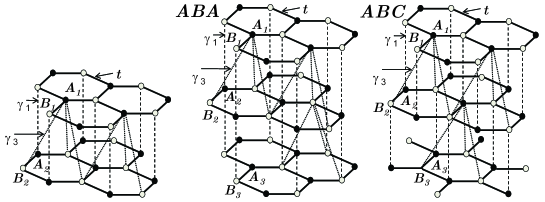
Figure 1: Atomic structure of bilayer, ABA- and ABC-stacked trilayer graphene.

In the present paper, we study the effect of different types of impurities on the transport properties of graphene layers by direct numerical simulations in a framework of the single-electron tight-binding model. We consider four different types of defects: resonant (“hydrogen”) impurities, vacancies, Gaussian on-site potentials and Gaussian nearest carbon-carbon hoppings. The resonant impurities/vacancies and the centers of the Gaussian potentials/couplings are randomly introduced in the graphene layers. Our numerical calculations are based on the time-evolution method Hams2000 ; DeRaedt2008 ; Yuan2010 , i.e., the time-evolution of the wave functions according to the Schrödinger equation with additional averaging over a random superposition of basis states. The main idea is that by performing Fourier transform of various correlation functions, such as the wave function-wave function and current-current correlation functions (Kubo formula), one can calculate the electronic structure and transport properties such as the density of states (DOS), quasieigenstates, ac (optical) and dc conductivities. The details of the numerical method are presented in Ref. Yuan2010, . The advantages of the time-evolution method is that it allows us to carry out calculations for very large systems, up to hundreds of millions of sites, with a computational effort that increases only linearly with the system size.

The paper is organized as follows. Section II gives a description of the tight-binding Hamiltonian of multilayer graphene. In section III, IV, V and VI, we focus on four different types of disorders respectively: resonant impurities, vacancies, potential impurities, and nearest carbon-carbon hopping impurities. Finally a brief discussion is given in section VII.

II Tight-binding model

In general, the tight-binding Hamiltonian of multilayer graphene is given by

$$H=\sum_{l=1}^{N_{layer}}H_{l}+\sum_{l=1}^{N_{layer}-1}H_{l}^{\prime},$$

where $H_{l}$ is the Hamiltonian of SLG for $l$’th layer and $H_{l}^{\prime}$ describes the hopping between layers $l$ and $l+1$.

The single-layer Hamiltonian $H_{l}$ is given by

$$H_{l}=H_{0}+H_{v}+H_{imp},$$ (1)

where $H_{0}$ derives from the nearest neighbor hopping between the carbon atoms:

$$H_{0}=-\sum_{<i,j>}t_{ij}c_{i}^{+}c_{j},$$ (2)

$H_{v}$ denotes the on-site potential of the carbon atoms:

$$H_{v}=\sum_{i}v_{i}c_{i}^{+}c_{i},$$ (3)

and $H_{imp}$ describes the resonant impurities (adatoms or admolecules):

$$H_{imp}=\varepsilon_{d}\sum_{i}d_{i}^{+}d_{i}+V\sum_{i}\left(d_{i}^{+}c_{i}+H.c.\right).$$ (4)

The interlayer Hamiltonian $H_{l}^{\prime}$ of bilayer graphene with AB Bernal stacking is given by

$$H_{l}^{\prime}=-\gamma_{1}\sum_{j}\left[a_{l,j}^{+}b_{l+1,j}+H.c.\right]-\gamma_{3}\sum_{j,j^{\prime}}\left[b_{l,j}^{+}a_{l+1,j^{\prime}}+H.c.\right],$$ (5)

where $a_{m,i}^{+}$ ($b_{m,j}$) annihilates an electron on sublattice A (B), in plane $m=l,l+1$, at site $R$ (see the atomic structure in Fig. 1). Thus, the second layer in BLG is rotated with respect to the first one by $+120^{\circ}$. For the third layer there are two options: either the third carbon layer will be rotated with respect to the second layer by $-120^{\circ}$ (than it will be exactly under the first layer) or by $+120^{\circ}$. In the first case we have ABA-stacked trilayer graphene, and in the second we have ABC-stacked (rhombohedral) graphene. The atomic structures of the ABA- and ABC-stacked trilayer graphene are shown in Fig. 1. These stacked sequences can be extended to multilayers, i.e., the direct extension of ABA- and ABC-stacked sequences from trilayer to quartic-layer are ABAB and ABCD. The spin degree of freedom contributes only through a degeneracy factor and, for simplicity, is omitted in Eq. (1).

The density of states is obtained by Fourier transformation of the wave function at time zero and time $t$:

$$\rho\left(\varepsilon\right)=\frac{1}{2\pi}\int_{-\infty}^{\infty}e^{i\varepsilon t}\left\langle\varphi\left(0\right)|\varphi\left(t\right)\right\rangle dt,$$ (6)

where $\left|\varphi\left(0\right)\right\rangle$ is an initial random superposition state of all the basis states and $\left|\varphi\left(t\right)\right\rangle=e^{-iHt}\left|\varphi\left(0\right)\right\rangle$ is calculated numerically according to the time-dependent Schrödinger equation (we use units with $\hbar=1$). A detailed description of this method can be found in Refs. Hams2000, ; Yuan2010, . The charge density is obtained by the intergral of the density of states, i.e., $n_{e}\left(E\right)=\int_{0}^{E}\rho\left(\varepsilon\right)d\varepsilon.$

The static (dc) conductivity is calculated by using the Kubo formula

$$\mathbf{\sigma}=-\frac{1}{A}Tr\left\{\frac{\partial f}{\partial H}\int_{0}^{\infty}dt\frac{1}{2}\left[JJ\left(t\right)+J\left(t\right)J\right]\right\}.$$ (7)

where $J$ is the current operator and $A$ is the sample area. The main idea of the calculation is to perform the time evolution of $\left|\varphi\left(0\right)\right\rangle$. Then, we can extract not only the DOS but also the quasieigenstates $\left|\Psi\left(\varepsilon\right)\right\rangle$ Yuan2010 , which are superpositions of degenerated energy-eigenstates. The conductivity at zero temperature can be represented as

$$\mathbf{\sigma}=\frac{\rho\left(\varepsilon\right)}{V}\int_{0}^{\infty}dt\text{Re}\left[e^{-i\varepsilon t}\left\langle\varphi\left(0\right)\right|Je^{iHt}J\left|\varepsilon\right\rangle\right],$$ (8)

where $\left|\varepsilon\right\rangle$ is defined as

$$\left|\varepsilon\right\rangle=\frac{1}{\left|\left\langle\varphi\left(0\right)|\Psi\left(\varepsilon\right)\right\rangle\right|}\left|\Psi\left(\varepsilon\right)\right\rangle.$$ (9)

The accuracy of the numerical results is mainly determined by three factors: the time interval of the propagation, the total number of time steps, and the size of the sample. In the numerical calculations, the integrals in Eq. (6) and (8) are calculated using the Fast Fourier Transform (FFT). According to the Nyquist sampling theorem, employing a sampling interval $\Delta t=\pi/\max_{i}\left|E_{i}\right|$, where $E_{i}$ are the eigenenergies, is sufficient to cover the full range of eigenvalues. In practice, we do not know $\max_{i}\left|E_{i}\right|$ exactly but it is easy to compute an upperbound (for instance the 1-norm of $H$) such that $\Delta t$ can be considered as fixed.

In the present paper, the time evolution is calculated by the Chebyshev polynomial method, which has the same accuracy as the machine’s precision independent of the value of time interval $\Delta t$. Alternatively, one could use Suzuki’s product formula decomposition of the exponential operators for the tight-binding Hamiltonian Kawarabayashi1995 , introducing another time step that has to be (much) smaller than $\Delta t$ to obtain accurate results Hams2000 . In both cases, the accuracy of the energy eigenvalues is determined by the total number of the propagation time steps $(N_{t})$ that is the number of the data items used in the FFT. Eigenvalues that differ less than $\Delta E=\pi/N_{t}\Delta t$ cannot be identified properly. However, since $\Delta E$ is proportional to $N_{t}^{-1}$ we only have to extend the length of the calculation by a factor of two to increase the accuracy by the same factor.

The third factor which determines the accuracy of our numerical results is the size of the sample. A sample with more sites in the real space will have more random coefficients in the initial state $\left|\varphi\left(0\right)\right\rangle$, providing a better statistical representation of the superposition of all energy eigenstates. This, however, is not a real issue in practice as it has be shown that the statistical fluctuations vanish with the inverse of the dimension of the Hilbert space Hams2000 , which for our problem, is proportional to the number of sites in the sample. A comparison of the DOS calculated from different samples size was shown in Ref. Yuan2010, , which clearly shows that larger sample size leads to better accuracy, and the result calculated from a SLG with $4096\times 4096$ lattice sites matches very well with the analytical expression Yuan2010 . More details on the numerical method itself can be found in Ref. Yuan2010, . The values of conductivity presented in this paper are normalized per layer and are expressed in units $e^{2}/h$.

Obviously, computer memory and CPU time evidently limit the size of the graphene system that can be simulated. The required CPU time is mainly determined by the number of operations to be performed on the state of the system, but this imposes no hard limit. However, the memory of the computer does. In the tight-binding approximation, a state $\left|\varphi\right\rangle$ of a sample consisting by $N_{c}$ atoms is represented by a complex-valued vector of length $D=N_{c}$. For numerical accuracy (and in view of the large number of arithmetic operators performed), it is advisable to use $13-15$ digit floating-point arithmetic (corresponding to $8$ bytes per real number). Thus, to represent the state $\left|\varphi\right\rangle$ we need at least $N_{c}\times 2^{4}$ bytes. For example, for $N_{c}=4096\times 4096\sim 1.6\times 10^{7}$ we need $256$ MB of memory to store a single arbitrary state $\left|\varphi\right\rangle$. This amount of memory is not a problem for the calculation of DOS on a modest desktop PC or notebook, but it limits the calculation of the dc conductivity on such machines. To calculate one value of $\sigma\left(\varepsilon\right)$ one needs storage of the corresponding quasieigenstate $\left|\varepsilon\right\rangle$, and with typically $64$ of such quasieigenstates in our simulations, a sample of $N_{c}=4096\times 4096$ sites requires at least $16$ GB memory for the storage, which is still reasonable for present-day computer equipment.

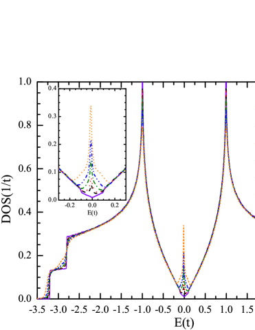
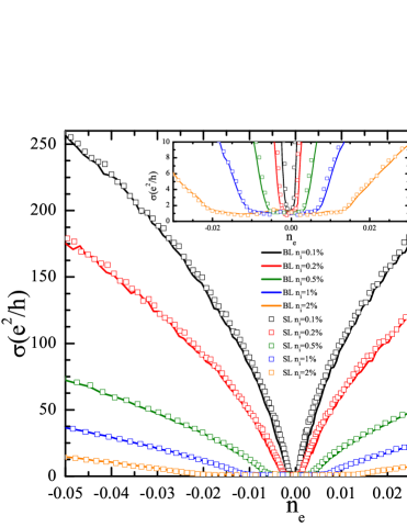
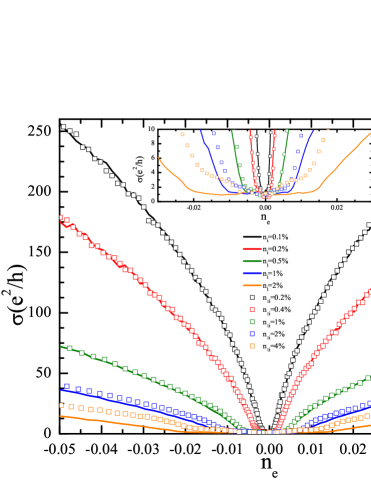
Figure 2: (Colour online) Top panel: DOS of bilayer graphene ($\gamma_{1}=\gamma_{3}=0.1t$) with different concentrations of resonant impurities ($\varepsilon_{d}=-t/16,$ $V=2t$) added on both layers. Middle panel: Comparison of the conductivity of the BLG (line) and SLG (square) with the same concentration of resonant impurities. Bottom panel: Comparison of the conductivity of bilayer graphene ($\gamma_{1}=\gamma_{3}=0.1t$) with the same amount of resonant impurities ($\varepsilon_{d}=-t/16,$ $V=2t$) added on both layers (line, $n_{i}$) or only one layer (triangle, $n_{1i}$). Each layer in BLG contains $4096\times 4096$ carbon atoms, and SLG contains $6400\times 6400\,$carbon atoms.

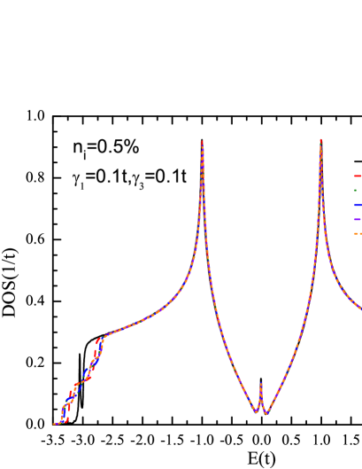
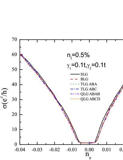
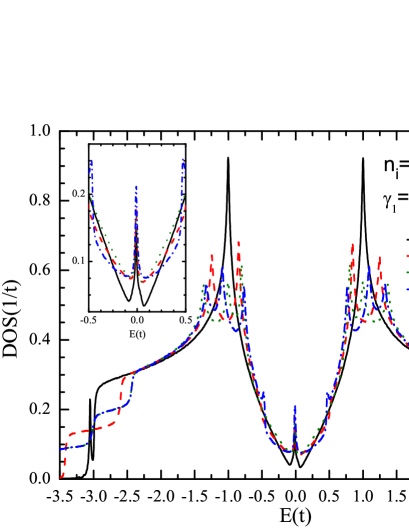
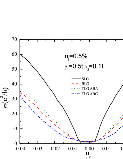
Figure 3: (Colour online) Comparison of the DOS and conductivity of the SLG, BLG, TLG and QLG with the same concentration of resonant impurities ($n_{i}=0.5\%$, $\varepsilon_{d}=-t/16,$ $V=2t$). $\gamma_{1}=\gamma_{3}=0.1t$ in top panels and $\gamma_{1}=0.5t,\gamma_{3}=0.1t$ in bottom panels. SLG contains $6400\times 6400\,$carbon atoms, each layer in BLG, TLG and QLG contains $4096\times 4096$, $3200\times 3200$ and $2400\times 2400$ carbon atoms, respectively.

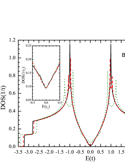
Figure 4: (Colour online) Comparison of the DOS of bilayer graphene with different interlayer interactions: $\gamma_{1}=0.1t$, $0.2t$, and $0.5t$ ($\gamma_{3}$ is fixed as $0.1t$). Inner panel: normalized DOS and energy in units of $1/\gamma_{1}$ and $\gamma_{1}$. Each layer in BLG contains $4096\times 4096$ carbon atoms.

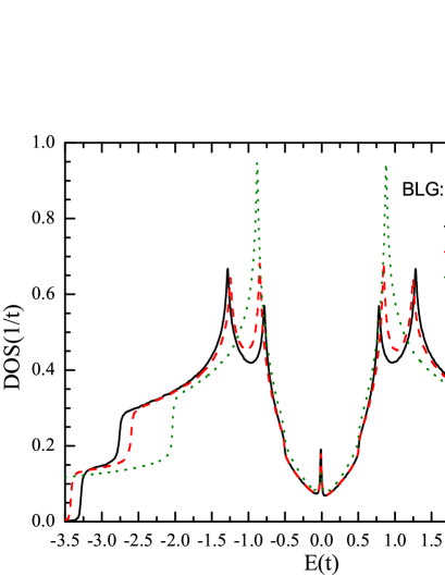
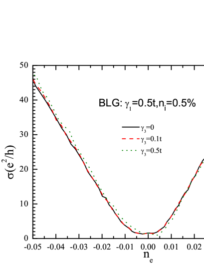
Figure 5: (Colour online) DOS and conductivity of bilayer graphene with resonant impurities ($\varepsilon_{d}=-t/16,$ $V=2t$) added on both layers. The interlayer parameter $\gamma_{1}$ is fixed as $0.5t$, and $\gamma_{3}=0$ (black line), $0.1t$ (red dashed line) and $0.5t$ (green dot line). Each layer contains $4096\times 4096$ carbon atoms.

III Resonant impurities

Resonant impurities are introduced in reality by the formation of a chemical band between a carbon atom from graphene sheet and a carbon atom from an adsorbed organic molecule (CH₃, C₂H₅, CH₂OH), as well as H atoms Wehling2010 ; vacancies are another option but in natural graphene their concentration seems to be small. The adsorbates are described by the Hamiltonian $H_{imp}$ in Eq. (1). From ab initio density functional theory (DFT) calculations Wehling2010 , it follows that the band parameters for various organic groups (and for hydrogen atoms) are almost the same: $V\approx 2t$ and $\epsilon_{d}\approx-t/16$. The hybridization strength $V$ being a factor $2$ larger than $t$ is in accordance with the hybridization for hydrogen adatoms from Ref. Robinson2008, , but the on-site energies $\epsilon_{d}$ are significantly smaller than the value $\epsilon_{d}$ $=1.7eV$ used for H in Ref. Robinson2008, which makes our results for the transport properties in SLG qualitatively different Wehling2010 ; Yuan2010 . The adoption of these band parameters successfully explained the resonant scattering in SLG Wehling2010 ; Yuan2010 and we continue to use them in the modeling of BLG and TLG.

In Refs. Wehling2010, ; Yuan2010, , we used the algorithm presented in the previous section to calculate the dc conductivity of SLG with resonant impurities or vacancies. We found that there is plateau of the order of the minimum conductivity Katsnelson2006 $4e^{2}/\pi h$ in the vicinity of the neutrality point, in agreement with theoretical expectations Ostrovsky2010 . Beyond the plateau, the conductivity is inversely proportional to the concentration of the impurities, and approximately proportional to the carrier concentration $n_{e}$. This is consistent with the approach based on the Boltzmann equation, which in the limit of resonant impurities with $V\rightarrow\infty$, yields for the conductivity Katsnelson2007 ; Katsnelson2008 ; Robinson2008 ; Wehling2010

$$\sigma\approx(2e^{2}/h)\frac{2}{\pi}\frac{n_{e}}{n_{i}}\ln^{2}\left|\frac{E_{F}}{D}\right|,$$ (10)

where $n_{e}=E_{F}^{2}/D^{2}$ is the number of charge carriers per carbon atom, and $D$ is of order of the bandwidth. Note that for the case of the resonance shifted with respect to the neutrality point the consideration of Ref. Katsnelson2007, leads to the dependence

$$\sigma\propto\left(q_{0}\pm k_{F}\ln{k_{F}R}\right)^{2},$$ (11)

where $\pm$ corresponds to electron and hole doping, respectively, and $R$ is the effective impurity radius. The Boltzmann approach does not work near the neutrality point where quantum corrections are dominant Ostrovsky2006 ; Katsnelson2006 ; Auslender2007 . In the range of concentrations, where the Boltzmann approach is applicable, our numerical results of the conductivity of SLG as a function of energy fits very well to the dependence given by Eq. (11) Wehling2010 ; Yuan2010 .

Electron scattering in BLG has been proven to differ essentially from SLG in Ref. Katsnelson_bilayer, : For a scattering potential with radius much smaller than the de Broglie wavelength of electrons, the phase shift of $s$-wave scattering $\delta_{0}$ tends to a constant as $k\rightarrow 0$. Therefore, within the limit of applicability of the Boltzmann equation, the conductivity of a bilayer should be just linear in $n_{e}$, instead of sublinear dependence (11) for SLG. The difference is that in SLG, due to vanishing DOS at the Dirac point, the scattering disappears at small wave vectors as $\delta_{0}(k)\propto 1/\ln{kR}$ (with $\ln^{2}{kR}$ on the order of 10 for typical amounts of doping) for resonant and as $\delta_{0}(k)\propto kR$ for the nonresonant impurities. In contrast, in BLG there are no restrictions on the strength of the scattering and even the unitary limit ($\delta_{0}=\pi/2$) can be reached at $k=0$.

However, these conclusions are based on the use of an approximate parabolic spectrum for the bilayer which is valid for the energy interval

$$|E|\ll|\gamma_{1}|.$$ (12)

In the opposite case

$$|E|\gg|\gamma_{1}|$$ (13)

the effects of the interlayer hopping are negligible and one should expect a behavior of the conductivity similar to that of SLG.

Our first set of numerical calculations of BLG are performed for similar concentrations of resonant impurities ($n_{i}\in[0.1\%,2\%]$) as those used for SLG in Refs. Wehling2010, ; Yuan2010, . The interlayer hopping parameters are taken as falko2006 $\gamma_{1}=\gamma_{3}=0.1t$. As shown in Fig. 2, finite concentrations of the resonant impurities lead to the formation of a low energy impurity band (see increased DOS at low energies in Fig. 2). The impurity band can host two electrons per impurity, and for impurity concentrations in the range of $[0.1\%,2\%]$, this leads to a plateau-shaped minimum of width $2n_{i}$ in the conductivity vs. $n_{e}$ curves around the neutrality point. As one can see from the DOS in Fig. 2, even for $n_{i}=0.1\%$, the width of the impurity band around the neutrality point is comparable to the limits of applicability of the parabolic approximation for the spectrum (12), therefore for the concentrations of the impurities presented in Fig. 2 one cannot use the theory Katsnelson_bilayer . For small electron concentrations we are beyond the limit of the Boltzmann theory at all, and for the larger electron concentration we are, rather, in the regime (13) so one could expect a sublinear behavior similar to that in SLG. Indeed, the conductivity of BLG as a function of charge density $n_{e}$ follows almost exactly the same dependence as for the SLG (see the direct comparisons of conductivities in Fig. 2). That is, the density-dependence of conductivity in BLG is not linear but sublinear (11) as in SLG. Actually, as shown in Fig. 3, the sublinear dependence is quite general for multilayer graphene, i.e., it is also true for trilayer and quartic-layer graphene with the same concentration of resonant impurities, independent on the stacking sequence, which is, of course, not surprising assuming that the condition (13) holds. Here for the trilayer (quartic-layer) we consider two types of stacking sequence: ABA (ABAB) and ABC (ABCD). This general property of the conductivity can be easily understood by comparison of their DOS in Fig. 3. The DOS of single-layer, bilayer, trilayer and quartic-layer graphene are exactly the same except near the edge of the spectrum, indicating the similar band structure, independent on the number of layers and stacking sequence. In fact, since the couplings between the carbon atoms and organic admolecules are twenty times larger than the interlayer coupling ($V=20\gamma_{1}$) in our model, the unique bonds generated by the relevant weaker interlayer interactions are more easily to be destroyed by the impurity bonds generated by the much stronger adsorbed resonant impurities.

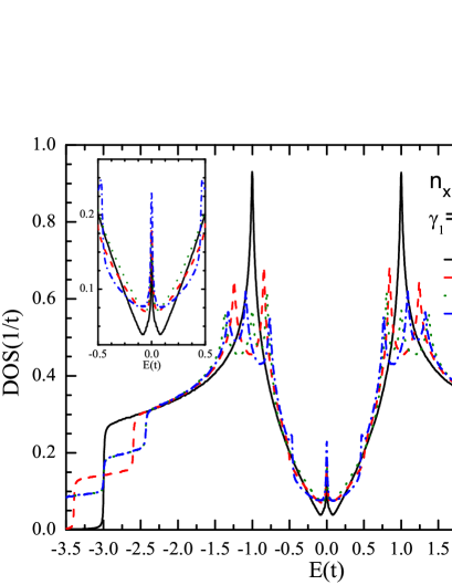
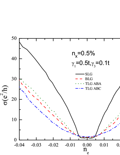
Figure 6: (Colour online) Comparison of the DOS and conductivity of the SLG, BLG and TLG with the same concentration of vacancies ($n_{x}=0.5\%$). The parameters of the interlayer coupling are $\gamma_{1}=0.5t$ and $\gamma_{3}=0.1t$. SLG contains $6400\times 6400\,$carbon atoms, each layer in BLG and TLG contains $4096\times 4096$ and $3200\times 3200$ carbon atoms (sites), respectively.

In order to check the symmetry of the presence of the impurities, we limit the adsorption of organic admolecules to one layer of BLG ($n_{1i}$, case II). To compare the results of the adsorption on both sides ($n_{i}$, case I), we fix the total number of resonant impurities and therefore the concentration on one layer (case II) is doubled ($n_{1i}=N_{imp}/N_{carbon\_in\_one\_layer}=2n_{i}$). We find (see last panel in Fig. 2) that for the low concentration ($n_{i}\leq 0.5\%$), the electron-density dependence of the conductivity in BLG follows the same law in both cases; at high concentration ($n_{i}\geq 1\%$), the conductivity in case II is larger than in case I. This is because in case II the difference of mobility of electron in the two layers, with or without impurities, is larger than in the case of large concentrations of adsorbed admolecules.

Next we consider the region of parameters which can be described by the Boltzmann equation plus parabolic spectrum Katsnelson_bilayer . In BLG, the approximations of massive valence and conduction bands with zero gap: $E\left(k\right)=\pm\hbar^{2}k^{2}/2m^{\ast}$, where the effective mass is given by $m^{\ast}=\gamma_{1}/2v_{F}^{2}$, are only true in the low-energy dispersion close to the neutrality point. There are two ways to place the impurity bands within the region of low-energy dispersion (12): decreasing the concentration $n_{i}$ of impurities or expanding the quadratic band by increasing $\gamma_{1}$. Smaller concentration of impurities leads to less random states for the averaging in the Kubo formula of Eq. (8), which means that it is numerically more expensive because we need to extend the sample size to keep the same accuracy. Therefore increasing $\gamma_{1}$ is computationally more convenient from the point of view of CPU time and physical memory; one can assume that physical results should be the same: it is only the ratio $n_{i}/\gamma_{1}$ which is important.

In Fig. 4, we compare numerical results of DOS of BLG with different band parameter $\gamma_{1}$: $0.1t,0.2t$ and $0.5t$ ($\gamma_{3}$ is fixed as $0.1t$). One can see that the width of the parabolic band with the energy-independent local density of states proportional to $\gamma_{1}$, and the normalized energy (in units of $\gamma_{1}$) dependencies of DOS (in the units of $1/\gamma_{1}$) within the parabolic band are consistent for different $\gamma_{1}$ (see the inner panel of Fig. 4). Therefore we can simply use $\gamma_{1}$ with the value of $0.5t$ instead of $0.1t$ to extend the width of the parabolic band approximation without changing the structure of the spectrum. The numerical results form a system with $m$ times larger of $\gamma_{1}$, are qualitatively comparable to those for a system of $1/m$ times smaller concentration $n_{i}$ of impurities.

The numerical results for the DOS and conductivities of BLG and TLG in the presence of resonant impurity with larger interlayer interactions ($\gamma_{1}=0.5t,$) are shown in Fig. 3. We see that for an impurity concentration of $n_{i}=0.5\%$, the impurity band is located around the neutral point and far from the edge of the quadratic band ($\left|E\right|<0.5t$). In the region of the impurity band ($|n_{e}|\leq n_{i}=0.5\%$), there is a plateau in the order of $2e^{2}/h$ (per layer) in BLG, as well as in TLG. This values is slightly larger than the minimum conductivity $4e^{2}/\pi h$ of SLG. It is worthwhile to note that an explanation of the origin of plateau around the neutrality point is beyond the applicability of Boltzmann equation, just as in the case of SLG Wehling2010 ; Yuan2010 . Analyzing experimental data of the plateau width (similar to the analysis for N₂O₄ acceptor states in Ref. Wehling2008, ) can therefore yield an independent estimate of the impurity concentration, both in single-layer and multilayer graphene. Within the parabolic band but beyond the impurity band, the conductivities in BLG and ABA-stacked TLG exhibit very well the linear dependence on the charge density $n_{e}$. The ABC-stacked TLG is different from the others because of its unique band structures with a cubic touching of the bands r3 (see the difference of DOS in Fig. 3).

Finally we check the role of $\gamma_{3}$ in the conductivity of BLG. Theoretically, the influence of $\gamma_{3}$ to the band structure is negligible, and so it is for the conductivity. This is confirmed by our numerical results in Fig. 5. For the fixed concentration of impurities $n_{i}=0.5\%$ with $\gamma_{1}=0.5t$, the values of the conductivity corresponding to the same electron concentration $n_{e}$ are quite close for $\gamma_{3}=0$, $0.1t$, and $0.5t$.

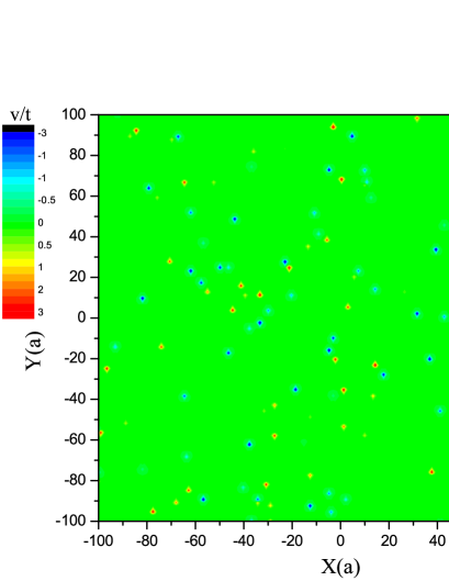
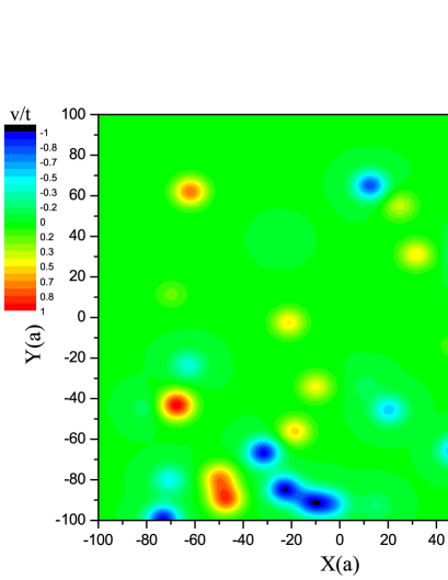
Figure 7: (Colour online) Contour plot of the on-site potentials in the central part of a graphene layer ($4096\times 4096$) with short-range ($\Delta=3t,$ $d=0.65a,$ $P_{v}=0.5\%$) or long-range ($\Delta=1t,$ $d=5a,$ $P_{v}=0.1\%$) Gaussian potential.

IV Vacancies

A vacancy in a graphene sheet can be regarded as an atom (lattice point) with an on-site energy $v\rightarrow\infty$ or with its hopping parameters to other sites being zero. In the numerical simulation, the simplest way to implement a vacancy is to remove the atom at the vacancy site. Introducing vacancies in SLG will create a zero energy modes (midgap state) Peres2006 ; Pereira2006 ; Pereira2008 ; Wehling2010 ; Yuan2010 . The exact analytical wave function associated with the zero mode induced by a single vacancy in SLG was obtained in Ref. Pereira2006, , showing a quasilocalized character with the amplitude of the wave function decaying as inverse distance to the vacancy. SLG with a finite concentration of vacancies was studied numerically in Refs. Peres2006, ; Pereira2008, ; Wehling2010, ; Yuan2010, ; Jafri2010, ; Chang2010, ; Wu2010, . It was shown that the number of the midgap states increases with the concentration of the vacancies Peres2006 ; Pereira2008 ; Wehling2010 ; Yuan2010 , and quasieigenstates are also quasilocalized around the vacancies Yuan2010 . The inclusion of vacancies brings an increase of spectral weight to the surrounding of the Dirac point ($E=0)$ and smears the van Hove singularities Peres2006 ; Pereira2008 ; Wehling2010 ; Yuan2010 . The effect of the vacancies on the transport properties of SLG is quite similar to that of the adsorbed organic molecules. The main difference is the position of the impurity band in the spectrum: its center is located at the neutrality point in the presence of vacancies, whereas it is biased in the presence of realistic resonant impurities because of the nonzero on-site potential on the organic carbon (or hydrogen) atom. The vacancy band contributes to the conductivity and leads to a plateau of minimum conductivity in the midgap region. The width of the plateau is $2n_{x}$ ($n_{x}$ is the concentration of the vacancies) in the conductivity vs. $n_{e}$ curves around the neutrality point, showing the same dependence ($2n_{i}$) as the case of resonant impurities Wehling2010 ; Yuan2010 . For the range of concentrations where the Boltzmann approach is applicable, the conductivity of SLG as a function of energy fits very well to the dependence given by Eq. (11), with $q_{0}=0$ for the vacancies and $q_{0}\neq 0$ for the resonant impurities Wehling2010 ; Yuan2010 .

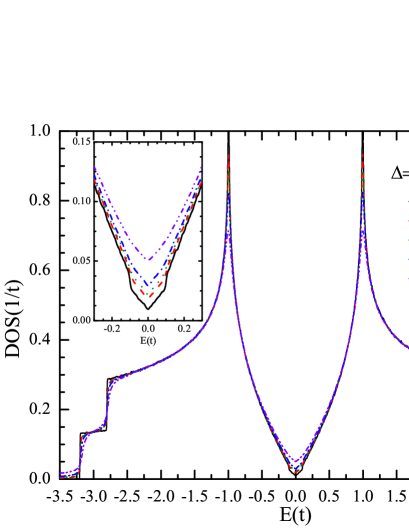
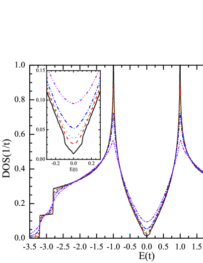
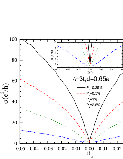
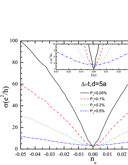
Figure 8: (Colour online) DOS and conductivity of bilayer graphene ($\gamma_{1}=\gamma_{3}=0.1t$) with short-range ($\Delta=3t,$ $d=0.65a$) or long-range ($\Delta=1t,$ $d=5a$) Gaussian potential. Each layer contains $4096\times 4096$ carbon atoms.

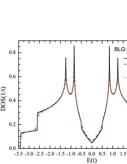
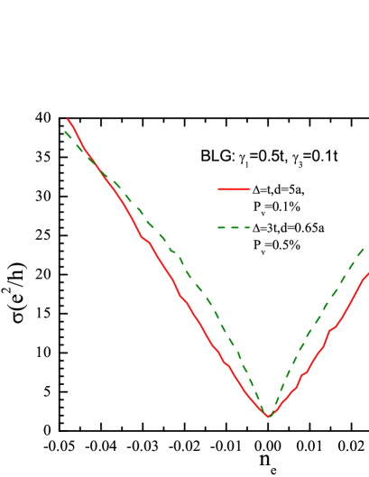
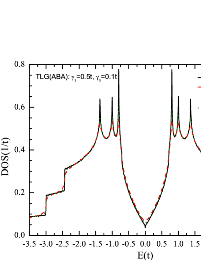
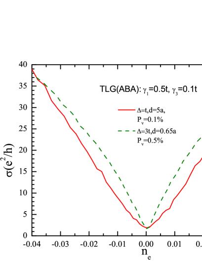
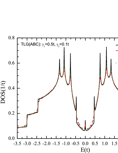
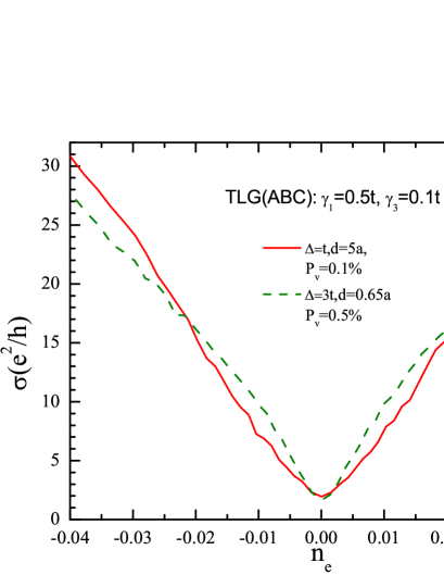
Figure 9: (Colour online) DOS and conductivity of bilayer graphene ($\gamma_{1}=0.5t$, $\gamma_{3}=0.1t$) with long-range ($\Delta=1t,$ $d=5a$) or short-range ($\Delta=3t,$ $d=0.65a$) Gaussian potential. Each layer contains $4096\times 4096$ carbon atoms.

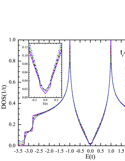
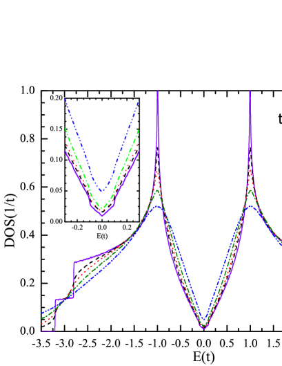
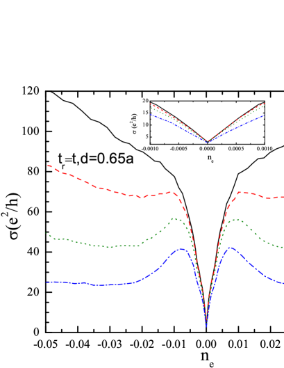
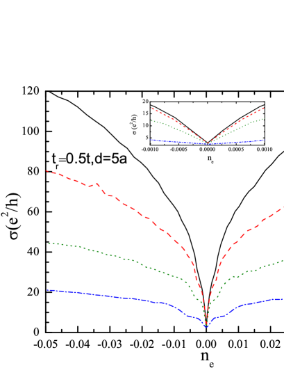
Figure 10: (Colour online) DOS and conductivity of bilayer graphene ($\gamma_{1}=\gamma_{3}=0.1t$) with short-range ($\Delta_{t}=t,$ $d_{t}=0.65a$) or long-range ($\Delta_{t}=0.5t,$ $d_{t}=5a$) Gaussian hopping. Each layer contains $4096\times 4096$ carbon atoms.

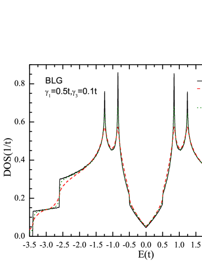
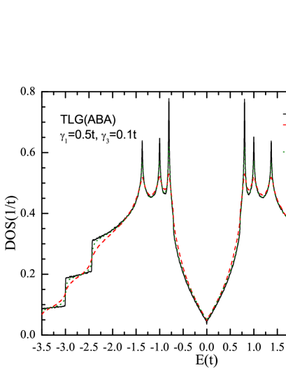
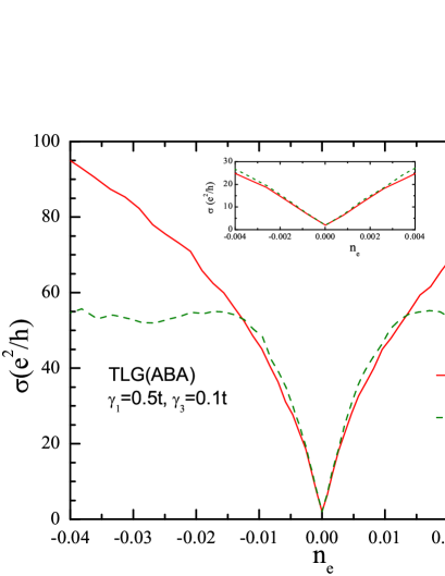
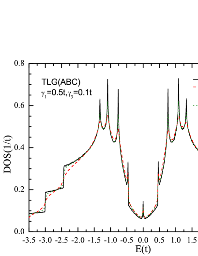
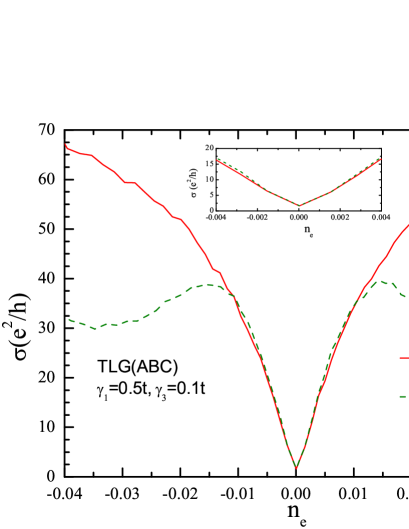
Figure 11: (Colour online) DOS and conductivity of bilayer graphene ($\gamma_{1}=\gamma_{3}=0.1t$) with short-range ($\Delta_{t}=t,$ $d_{t}=0.65a$) or long-range ($\Delta_{t}=0.5t,$ $d_{t}=5a$) Gaussian hopping. Each layer contains $4096\times 4096$ carbon atoms.

Previous studies of the vacancies in BLG focused mainly on the properties of the local density of states (LDOS) around a single or a pair of vacancies, and it was shown that the LDOS in the neighboring lattice sites of the impurity site is normally enhanced, depending on the lattice site (A or B sublattices) of the vacancy Wang2007 ; Dahal2008 . Recently, a new type of zeromodel state in BLG is found in Ref. Castro2010b, , in the absence of a gap it is quasilocalized in one of the layers and delocalized in the other, and in the presence of a gap it becomes fully localized inside the gap. These observations are different from SLG, where the impurity state is insensitive to the position of vacancies. The differences in the spectrum of LDOS around the vacancies in SLG and BLG lead to different electron-density (Fermi energy) dependence of the conductivity. As the vacancies and resonant impurities have similar effects on the electronic structure and transport properties in SLG Wehling2010 ; Yuan2010 , it suggests that their contributions to the bilayer and trilayer graphene should also be comparable. We consider here the results for the vacancies in the range that the Boltzmann approach is applicable. In Fig. 6, we show the numerical results of the DOS and conductivities of SLG, BLG and TLG with fixed concentration of vacancies ($n_{x}=0.5\%$). The parameters of the interlayer coupling are $\gamma_{1}=0.5t$ and $\gamma_{3}=0.1t$. These results are directly comparable with the results of the same concentration of resonant impurities represented in Fig. 3, and demonstrate similar density-dependence of the conductivities, just as we expected. For conciseness, we do not discuss these vacancies as their effect on the transport properties of graphene are quite similar to those of the resonant impurities.

V Gaussian Potential

The impurities in the Hamiltonian of Eq. (1) are represented by random on-site potentials. Short-rang and long-range Gaussian potentials are given by

$$v_{i}=\sum_{k=1}^{N_{imp}^{v}}U_{k}\exp\left(-\frac{\left|\mathbf{r}_{i}-\mathbf{r}_{k}\right|^{2}}{2d^{2}}\right),$$ (14)

where $N_{imp}^{v}$ is the number of the Gaussian centers, which are chosen randomly distributed on the carbon atoms, $U_{k}$ is uniformly random in the range $[-\Delta,\Delta]$ and $d$ is interpreted as the effective potential radius. The typical values of $d$ used in our model are $d=0.65a$ and $5a$ for short- and long-range Gaussian potential, respectively. Here $a$ is the carbon-carbon distance in the monolayer graphene. The value of $N_{imp}^{v}$ is characterized by the value $P_{v}=N_{imp}^{v}/N$, where $N$ is the total number of carbon atoms of the sample. A typic contour plot of the on-site potentials in the central part of a graphene layer with short- or long-range Gaussian potential is shown in Fig. 7. The sum in Eq. (14) is limited to the sites in the same layer, i.e., we do not consider the overlapping of the Gaussian distribution in different layers.

Numerical results of the density of states and dc conductivities of BLG ($\gamma_{1}=\gamma_{3}=0.1t$) with short- ($\Delta=3t,$ $d=0.65a$) and long-range ($\Delta=1t,$ $d=5a$) Gaussian potentials are shown in Fig. 8. Similar to the case of resonant impurities, the singularities in the spectrum are also suppressed in the presence of random potentials, and the conductivity as a function of charge density follows a sublinear dependence. The difference is that there is no impurity band around the neutrality point (see the DOS in Fig. 8). This leads to totally different transport properties: no plateau around the Dirac point in the conductivity vs. $n_{e}$ curves.

Similar to the case of resonant impurities, the regime of parabolic band in BLG expands by increasing $\gamma_{1}$ from $0.1t$ to $0.5t$, the results being shown in Fig. 9. Now the difference of transport properties in BLG with short- and long-range Gaussian potentials are more significant within the parabolic band: the density-dependence of conductivity is sublinear in the case of short-range, but linear in the case of long-range potentials. Actually, these sublinear and linear dependencies are also observed in TLG, independent on the stacking sequence (see Fig. 9).

The same value of the minimum conductivity ($\sigma_{\min}\approx 2e^{2}/h$) at the charge neutrality point is observed for both BLG and TLG with $\gamma_{1}=0.5t$. As we discussed in the case of resonant impurities, the adoption of larger $\gamma_{1}$ is equivalent to the use of smaller disorder, and therefore our results indicate that the minimum conductivity in order of $\sigma_{\min}\approx 2e^{2}/h$ is common in BLG and TLG with small concentration of random Gaussian potentials. These numerical results are consistent with the analytical result for BLG in Ref. Katsnelson_bilayer, .

VI Gaussian Hopping

The origin of disorder in the nearest neighbor coupling could be substitutional impurities like N or B instead of C, or distortions of graphene sheet. To be specific, we introduce the disorder in the hopping by a Gaussian distribution in a similar way as random Gaussian potential, namely, the distribution of the nearest neighbor hopping parameters reads

$$t_{ij}=t+\sum_{k=1}^{N_{imp}^{t}}T_{k}\exp\left(-\frac{\left|\mathbf{r}_{i}+\mathbf{r}_{j}-2\mathbf{r}_{k}\right|^{2}}{8d_{t}^{2}}\right),$$ (15)

where $N_{imp}^{t}$ is the number of the Gaussian centers, $T_{k}$ is uniformly random in the range $[-\Delta_{t},\Delta_{t}]$ and $d_{t}$ is interpreted as the effective screening length. Similarly, the typical values of $d_{t}$ are the same as for the Gaussian potential, i.e., $d_{t}=0.65a$ and $5a$ for short- and long-range Gaussian random hopping, respectively, and the values of $N_{imp}^{t}$ are characterized by the value $P_{t}=N_{imp}^{t}/N$. Similar as in Eq. (14), the sum in Eq. (15) does not include the overlapping of the Gaussian distribution in different layers.

Like in the case of Gaussian potentials, the presence of random Gaussian hopping in BLG and TLG also suppresses the Van Hove singularities in the spectrum, but does not introduce a new impurity band (midgap states) and there is also no plateau in the conductivity vs. electron density curves (see Fig. 10 and 11). The unique feature characteristic for the presence of random Gaussian hopping is that in the region near the neutrality point, the conductivity is always linearly dependent on the electron density, with no influence from the concentration of Gaussian centers (different $P_{t}$ in Fig. 10), range of Gaussian coupling ($d_{t}=0.65a$ or $5a$), strength of the interlayer coupling ($\gamma_{1}=0.1t$ in Fig. 10 and $0.5t$ in Fig. 11), number of layers (bilayer or trilayer) and stacking sequence (ABA or ABC in TLG). The differences of short- or long-range cases are only obvious in the energy region far from the neutrality point (high concentration of charge density): the increase of conductivity as a function of charge density is monotonic only for the long-range disorder. Furthermore, like in the case of random Gaussian potential, a common minimum conductivity in the order of $2e^{2}/h$ on charge neutrality point is also observed for both BLG and TLG.

VII Discussion and Conclusions

We have presented a detailed numerical study of the electronic transport properties of bilayer and trilayer graphene within the framework of a noninteracting tight-binding model. Various realistic types of disorder are considered, such as resonant impurities, vacancies, random Gaussian on-site potentials, and random Gaussian hopping between nearest carbon atoms. Our results give a consistent picture of the electronic structure and transport properties of bilayer and trilayer graphene in a broad range of concentration of impurities or other sources of disorder. Linear or sublinear electron-density dependent conductivity at high enough density is observed, depending on the type and strength of the disorder and the stacking sequence. The minimum conductivity $\sigma_{\min}\approx 2e^{2}/h$ (per layer) on charge neutrality point is common for BLG and TLG, independent of the type of the impurities, but the plateau of minimum conductivity around the neutrality point is unique when resonant impurities or vacancies are present.

In the presence of resonant impurities or vacancies, the dependence of the conductivity as a function of electron density is affected by the relevant width of the impurity band and the band created by the interlayer hopping. Using BLG with vacancies as an example: introducing $n_{p}\equiv n_{e}\left(\gamma_{1}\right)=\int_{0}^{\gamma_{1}}\rho\left(\varepsilon\right)d\varepsilon$ as the density of electrons on the boundary of the parabolic band, and considering the case that the concentration of vacancies ($n_{x}$) is smaller than $n_{p}$, i.e., the impurity band is within the region of the parabolic conduction band, there are three regions of electron-density dependence of the conductivity:

(i) $\left|n_{e}\right|\leq n_{x}$, a central minimum conductivity plateau ($2e^{2}/h$ per layer) with width equals to $2n_{x}$;

(ii) $n_{x}<\left|n_{e}\right|<n_{p}$, linear dependence, as predicted by the analytical treatment using the Boltzmann equation for parabolic spectrum Katsnelson_bilayer ;

(iii) $n_{x}\geq n_{p}$, sublinear dependence, as the effects of the interlayer hopping are negligible in this region and one should expect a behavior of the conductivity similar to that of SLG.

On the opposite case $n_{x}\geq n_{p}$, region (ii) simply disappears and therefore we can only observe the minimum conductivity plateau and sublinear dependence on the high concentration of electron densities. Actually, the sublinear dependence beyond the parabolic band is a general property of SLG, BLG and MLG with large enough concentration of resonant impurities or vacancies, independent on the number of layers and the stacking sequence.

In the presence of random Gaussian on-site potentials, the electron-density dependences of conductivity of BLG or TLG are sublinear and linear in the low concentration of charges, for short- and long-range disorders, respectively but are always sublinear in the high concentration. On the other hand, in the case of random Gaussian carbon–carbon couplings, the density-dependence of conductivity in the region close to the neutrality point is more simple: there is only a linear dependence, with no effect of the strength and range of disorder, the number of layers and stacking sequence.

Note added: After this paper was submitted, a paper which also discusses the effect of resonant scatterers on the dc conductivity of single-layer and bilayer graphene appeared Ferreira2010 , with results that are consistent with ours.

VIII Acknowledgement

The support by the Stichting Fundamenteel Onderzoek der Materie (FOM) and the Netherlands National Computing Facilities foundation (NCF) are acknowledged.

References

- (1) A. K. Geim and K. S. Novoselov, Nature Mater. 6, 183 (2007).
- (2) M. I. Katsnelson, Mater. Today 10, 20 (2007).
- (3) A. H. Castro Neto, F. Guinea, N. M. R. Peres, K. S. Novoselov, and A. K. Geim, Rev. Mod. Phys. 81, 109 (2009).
- (4) C. W. J. Beenakker, Rev. Mod. Phys. 80, 1337 (2008).
- (5) A. K. Geim, Science 324, 1530 (2009).
- (6) S. Das Sarma, S. Adam, E. H. Hwang, and E. Rossi, arXiv:1003.4731.
- (7) M. A. H. Vozmediano, M. I. Katsnelson, and F. Guinea, Phys. Rep. 496, 109 (2010).
- (8) A. Cresti, N. Nemec, B. Biel, G. Niebler, F. Triozon, G. Cuniberti, and S. Roche, Nano Research 1, 361 (2008).
- (9) E. R. Mucciolo and C. H. Lewenkopf, J. Phys.: Condens. Matter 22, 273201 (2010).
- (10) N. M. R. Peres, Rev. Mod. Phys. 82, 2673 (2010).
- (11) K. S. Novoselov, E. McCann, S. V. Morozov, V. I. Falko, M. I. Katsnelson, U. Zeitler, D. Jiang, F. Schedin, and A. K. Geim, Nature Phys. 2, 177 (2006).
- (12) E. McCann and V. I. Falko, Phys. Rev. Lett. 96, 086805 (2006).
- (13) F. Guinea, A. H. Castro Neto, and N. M. R. Peres, Phys. Rev. B 73, 245426 (2006).
- (14) T. Ohta, A. Bostwick, T. Seyller, K. Horn, E. Rotenberg, Science 313, 951 (2006).
- (15) E. McCann, Phys. Rev. B 74, 161403 (2006).
- (16) M. Koshino and T. Ando, Phys. Rev. B 73, 245403 (2006).
- (17) M. I. Katsnelson, Phys. Rev. B 76, 073411 (2007).
- (18) J. Nilsson, A. H. Castro Neto, F. Guinea, and N. M. R. Peres, Phys. Rev. Lett. 97, 266801 (2006).
- (19) J. Nilsson, A. H. Castro Neto, N. M. R. Peres, and F. Guinea, Phys. Rev. B 73, 214418 (2006).
- (20) J. Nilsson and A. H. Castro Neto, Phys. Rev. Lett. 98, 126801 (2007).
- (21) J. Nilsson, A. H. Castro Neto, F. Guinea, and N. M. R. Peres, Phys. Rev. B 78, 045405 (2008).
- (22) E. V. Castro, K. S. Novoselov, S. V. Morozov, N. M. R. Peres, J. M. B. Lopes dos Santos, J. Nilsson, F. Guinea, A. K. Geim, and A. H. Castro Neto, Phys. Rev. Lett. 99, 216802 (2007).
- (23) E. V. Castro, N. M. R. Peres, J. M. B. Lopes dos Santos, A. H. Castro Neto, and F. Guinea, Phys. Rev. Lett. 100, 026802 (2008).
- (24) J. M. B. Lopes dos Santos, N. M. R. Peres, and A. H. Castro Neto, Phys. Rev. Lett. 99, 256802 (2007).
- (25) P. Mallet, F. Varchon, C. Naud, L. Magaud, C. Berger, and J.-Y. Veuillen, Phys. Rev. B 76, 041403(R) (2007).
- (26) A. Bostwick, T. Ohta, J. L. McChesney, K. V. Emtsev, T. Seyller, K. Horn, and E. Rotenberg, New J. Phys. 9 385, (2007).
- (27) R. V. Gorbachev, F. V. Tikhonenko, A. S. Mayorov, D. W. Horsell, and A. K. Savchenko, Phys. Rev. Lett. 98, 176805 (2007).
- (28) Y. M. Lin and P. Avouris, Nano Lett., 8, 2119 (2008).
- (29) M. Nakamura, L. Hirasawa, and Ken-Ichiro Imura, Phys. Rev. B 78, 033403 (2008).
- (30) B. E. Feldman, J. Martin, and A. Yacoby, Nat. Phys. 5, 889 (2009).
- (31) M. Trushin, J. Kailasvuori, J. Schliemann, and A. H. MacDonald, Phys. Rev. B 82, 155308 (2010).
- (32) V. M. Pereira, R. M. Ribeiro, N. M. R. Peres, and A. H. Castro Neto, Phys. Rev. B 79, 045421 (2009).
- (33) S. V. Morozov, K. S. Novoselov, M. I. Katsnelson, F. Schedin, D. C. Elias, J. A. Jaszczak, and A. K. Geim, Phys. Rev. Lett. 100, 016602 (2008).
- (34) R. M. Ribeiro, N. M. R. Peres, J. Coutinho, and P. R. Briddon, Phys. Rev. B 78, 075442 (2008).
- (35) W. Zhu, V. Perebeinos, M. Freitag, and P. Avouris, Phys. Rev. B 80, 235402 (2009).
- (36) S. Das Sarma, E. H. Hwang, and E. Rossi, Phys. Rev. B 81, 161407 (2010).
- (37) M. Lv and S. Wan, Phys. Rev. B 81, 195409 (2010).
- (38) S. Xiao, J. Chen, S. Adam, E. D. Williams, and M. S. Fuhrer, Phys. Rev. B 82, 041406 (2010).
- (39) F. Zhang, B. Sahu, H. Min, and A. H. MacDonald, Phys. Rev. B 82, 035409 (2010).
- (40) W. Zhu, D. Neumayer, V. Perebeinos, and P. Avouris, Nano Letters 10 3572 (2010).
- (41) J. B. Oostinga, H. B. Heersche, X. Liu, A. F. Morpurgo, and L. M. K. Vandersypen, Nature Mater. 7, 151 (2008).
- (42) Y. Zhang, T.-T. Tang, C. Girit, Z. Hao, M. C. Martin, A. Zettl, M. F. Crommie, Y. Ron Shen, and F. Wang, Nature 459, 820 (2009).
- (43) E. V. Castro, K S Novoselov, S. V. Morozov, N. M. R. Peres, J. M. B. Lopes dos Santos, J. Nilsson, F. Guinea, A. K. Geim and A. H. Castro Neto, J. Phys.: Condens. Matter 22 175503 (2010).
- (44) T. Taychatanapat and P. Jarillo-Herrero, Phys. Rev. Lett. 105, 166601 (2010).
- (45) M. F. Craciun, S. Russo, M. Yamamoto, J. B. Oostinga, A. F. Morpurgo, S. Tarucha, Nature Nanotechnology, 4, 383 ( 2009).
- (46) M. Koshino and E. McCann, Phys. Rev. B 79, 125443 (2009).
- (47) N. H. Shon and T. Ando, J. Phys. Soc. Jpn. 67, 2421 (1998).
- (48) N. M. R. Peres, F. Guinea, and A. H. Castro Neto, Phys. Rev. B 73, 125411 (2006).
- (49) M. I. Katsnelson and K. S. Novoselov, Solid State Commun. 143, 3 (2007).
- (50) M. Hentschel and F. Guinea, Phys. Rev. B 76, 115407 (2007).
- (51) D. S. Novikov, Phys. Rev. B 76, 245435 (2007).
- (52) K. Nomura and A. H. MacDonald, Phys. Rev. Lett. 96, 256602 (2006).
- (53) T. Ando, J. Phys. Soc. Japan 75, 074716 (2006).
- (54) E. H. Hwang, S. Adam, and S. Das Sarma, Phys. Rev. Lett. 98, 186806 (2007).
- (55) S. Adama, E.H. Hwanga, E. Rossia and S. Das Sarma, Solid State Commun. 149, 1072 (2009).
- (56) M. I. Katsnelson and A. K. Geim, Phil. Trans. R. Soc. A 366, 195 (2008).
- (57) P. M. Ostrovsky, I. V. Gornyi, and A. D. Mirlin, Phys. Rev. B 74, 235443 (2006).
- (58) T. Stauber, N. M. R. Peres, and F. Guinea, Phys. Rev. B 76, 205423 (2007).
- (59) Z. H. Ni, L. A. Ponomarenko, R. R. Nair, R. Yang, S. Anissimova, I. V. Grigorieva, F. Schedin, P. Blake, Z. X. Shen, E. H. Hill, K. S. Novoselov, A. K. Geim, Nano Lett. 10, 3868 (2010).
- (60) M. Titov, P. M. Ostrovsky, I. V. Gornyi, A. Schuessler, and A. D. Mirlin, Phys. Rev. Lett. 104, 076802 (2010).
- (61) V. M. Pereira, F. Guinea, J. M. B. Lopes dos Santos, N. M. R. Peres, and A. H. Castro Neto, Phys. Rev. Lett. 96, 036801 (2006).
- (62) V. M. Pereira, J. M. B. Lopes dos Santos, and A. H. Castro Neto, Phys. Rev. B 77, 115109 (2008).
- (63) J. P. Robinson, H. Schomerus, L. Oroszlány, and V. I. Fal’ko, Phys. Rev. Lett. 101, 196803 (2008).
- (64) T. O. Wehling, S. Yuan, A. I. Lichtenstein, A. K. Geim, and M. I. Katsnelson, Phys. Rev. Lett. 105, 056802 (2010).
- (65) S. Yuan, H. De Raedt, M. I. Katsnelson, Phys. Rev. B 82, 115448 (2010).
- (66) T. Kawarabayashi and T. Ohtsuki, Phys. Rev. B 51, 10897 (1995).
- (67) S. H. M. Jafri, K. Carva, E. Widenkvist, T. Blom, B. Sanyal, J. Fransson, O. Eriksson, U. Jansson, H. Grennberg, O. Karis, R. A. Quinlan, B. C. Holloway and K. Leifer, J. Phys. D: Appl. Phys. 43, 045404 (2010).
- (68) S. Wu and F. Liu, arXiv:1001.2057v1.
- (69) Y. C. Chang and S. Haas, arXiv:1009.5941v1.
- (70) A. Hams and H. De Raedt, Phys. Rev. E 62, 4365 (2000).
- (71) H. De Raedt and M. I. Katsnelson, JETP Lett. 88, 607 (2008).
- (72) M. I. Katsnelson, Eur. Phys. J. B 51, 157 (2006).
- (73) M. Auslender and M. I. Katsnelson, Phys. Rev. B 76, 235425 (2007).
- (74) P. M. Ostrovsky, M. Titov, S. Bera, I. V. Gornyi, and A. D. Mirlin, arXiv:1006.3299.
- (75) T. Wehling, K. Novoselov, S. Morozov, E. Vdovin, M. I. Katsnelson, A. Geim, and A. Lichtenstein, Nano Letters 8, 173 (2008).
- (76) Z. Wang, Q. Li, H. Su, X. Wang, Q. Shi, J. Chen, J. Yang, and J. Hou, Phys. Rev. B 75, 085424 (2007).
- (77) H. P. Dahal, A. V. Balatsky, and J. X. Zhu, Phys. Rev. B 77, 115114 (2008).
- (78) E. V. Castro, M. P. Lopez-Sancho, and M. A. H. Vozmediano, Phys. Rev. Lett. 104, 036802 (2010).
- (79) A. Ferreira, J. Viana Gomes, J. Nilsson, E. R. Mucciolo, N. M. R. Peres, and A. H. Castro Neto, arXiv:1010.4026