Large random correlations in individual mean field spin glass samples

Abstract

We argue that complex systems must possess long range correlations and illustrate this idea on the example of the mean field spin glass model. Defined on the complete graph, this model has no genuine concept of distance, but the long range character of correlations is translated into a broad distribution of the spin-spin correlation coefficients for almost all realizations of the random couplings. When we sample the whole phase space we find that this distribution is so broad indeed that at low temperatures it essentially becomes uniform, with all possible correlation values appearing with the same probability. The distribution of correlations inside a single phase space valley is also studied and found to be much narrower.

1 Introduction

Spin glasses [1] and their (in many respects well understood) mean field versions, like the Sherrington-Kirkpatrick (SK) model [2], have emerged in the last decades as an interesting paradigm for complexity: indeed, they represent one of the few approaches to complexity where one can gain a good analytical and mathematical control. In these systems, with competing quenched random couplings inducing disorder and frustration, one has a phase transition to a low temperature spin glass phase. The critical temperature $T_{c}$ is characterized by a divergent correlation length, but, more remarkably, the whole ordered phase in the range $0\leq T\leq T_{c}$ is critical ($T$ is the temperature of the system): the presence of an infinite number of equilibrium states implies that, at all temperatures in the spin glass phase, the state to state transitions generate an infinite correlation length.

Broken continuous symmetries also lead to the appearance of zero modes all through the ordered phase of ordinary translationally invariant systems. No such continuous symmetry is present in the Ising spin glass however, and the mechanism of the generation of long range correlations is completely different from, say, the one induced by the long wavelength spin waves in the Heisenberg model. We believe that the multiattractor structure of the spin glass phase and the long range correlations generated by it are characteristic of many complex systems, and it is in this context that we wish to place the present work.

The idea that the spin glass phase is, in some sense, “soft” has been around from the very beginning of the field. The stability analysis of the Parisi solution for the SK model provided a proof for the existence of zero modes in the replica symmetry broken phase  [3]. The authors went on to calculate the various propagators in the first (Gaussian) correction to the mean field approximation of replica field theory, and found different power law like asymptotic behaviors, depending on the value of the replica overlap [4, 5]. Somewhat later, they presented a formally exact theorem for the existence of zero modes all through the replica symmetry broken phase [6], while further work clarified the connection between the spin glass propagators and the various overlap correlations that can be defined in the model, and worked out the long wavelength asymptotics of these correlation functions in the Gaussian approximation [7, 8]. Extensive numerical calculations found convincing evidence for these long range correlation functions in low dimensional spin glass models, although they also demonstrated the strong renormalization of some of the correlation exponents, with respect to the Gaussian approximation [9]. All the analytic studies cited so far took the “many valleys”, or “replica symmetry breaking” picture as their starting point. Remarkably, soft excitations and power law like behavior for the correlation functions are also an integral part of the rival droplet theory [10]. It seems therefore that, at least as far as the algebraic character of the long distance behavior of correlation functions is concerned, there is a rare general agreement between the various schools of thought.

Most of the analytic as well as numerical studies of spin glass correlations have focused on the behavior of quantities averaged over the quenched disorder . In the present work we propose to consider the simplest spin-spin correlations without averaging over the randomness. While the average of this object must be trivial, the individual samples must display a highly nontrivial correlation structure that has so far been dismissed as a legitimate object of study, on account of its random, chaotic character. We wish to study this object in the SK model not for its own sake, however, but as perhaps the simplest manifestation of the appearance of strong correlations generated by a complex phase space structure. Looking at the model from the point of view of real world complex systems whose dynamics depends on competing interactions (neural networks, complex optimization, the economy, the financial network, the power grid, traffic, etc.) we have to realize that these are usually large, but not infinitely large This means that their various subsystems cannot necessarily be expected to realize all the different samples of the random couplings, which invalidates the rationale for averaging over the randomness. In this context, it is therefore a most relevant question whether the various spin glass samples display some common characteristics that may be regarded as typical, and may be expected to show up also in other complex systems. In particular, we wish to look into the distribution of correlations and see how general the appearance of large random values is.

Let us start by recalling some facts about criticality and correlations. Ordinary, non-complex systems display short range correlations. Beyond a certain length scale the various parts of the system become independent of each other. This is the property behind ordinary thermodynamic behavior (e.g. extensive internal energy, thermal fluctuations of extensive quantities proportional to $\sqrt{N}$, etc.). An equivalent statement is that the probability density functions for the whole system approximately factorize into distributions belonging to (sufficiently large) subsystems. In the renormalization group (RG) framework, one has a renormalization group flow to a Gaussian, or high temperature fixed point. When, however, a system is complex and it “is more than the sum of its parts”, the above properties do not hold: in particular, correlations must be long ranged (see also the recent discussion in [15]).

An example of this type of behavior is the critical state. Correlations in the critical state decay like a power of the distance. In a usual, translationally invariant critical system, they decay monotonically. As for the ordered phase of an ordinary, translationally invariant system, its correlations, calculated over the full Gibbs ensemble, decay to a constant, and it is only within a pure phase that clustering holds and connected correlations vanish for large distances. We have said that the ordered phase of spin glasses is in some sense critical: it is reasonable then to ask what the behavior of correlations is in this case. What correlations do after averaging over randomness is well understood at the level of the Gaussian approximation [8]. Averaged squared correlations decay as power laws, and they decay monotonically. They show this behavior both in the full ensemble, and in the pure states, the individual valleys. This implies, and we are getting here close to the point we want to discuss, some kind of long-range behavior also for the correlations in a given sample: the average value of the self-overlap of correlations inside a given valley, taken at a fixed long distance, cannot be large without at least some of the sample correlations, taken at the same distance, being large. Hence, the correlations in the individual samples must be long ranged, in some sense. In what sense? The system is not translationally invariant, therefore there is no reason to expect that the correlations in the individual samples behave monotonically. They may drop over small distances, becoming large again somewhat farther away, may change sign a number of times along the way, and start to decay (in absolute value) for even longer distances. If these correlations are to be long ranged, they must take up large values with some probability even for very long distances.

This picture of the behavior of correlations in the pure phase of a spin glass says that large values of these correlations tend to cluster at small distances, but there is no monotonicity, and occasionally there are large correlations even between very far away partners. The probability of finding a strongly correlated pair at large distances is decaying with the distance, but there will always be strongly correlated pairs separated by very long distances. Averaging over these correlations one should be able to recover the known results (bearing in mind that the results [8] were derived in the Gaussian approximation). The existence of these long ranged correlations in every sample explains the curious behavior in the thermodynamic limit: adding another layer to even a very large system may reorganize the equilibrium distribution of spins inside the bulk, because large correlations may be generated between the old spins and the ones in the newly added layer. The existence of large correlations is then seen to be intimately related to the so called “chaos in system size”  [16]. For the same reason, due care must be taken when specifying boundary conditions in a simulation for spin glasses, and also when defining a real space renormalization procedure, for example. A broad range of correlations at all length scales has been found to appear in hierarchical lattices [17].

In this note we would like to understand what all this may imply for the Sherrington-Kirkpatrick (SK) model. We regard this model as the simplest laboratory where the phenomenon of large, random correlations, that we conjecture to be a generic feature of complex systems, can be studied.

Let us first consider a simple ferromagnetic Ising model (in a finite number of dimensions). Here if we are above the critical point the correlations decay exponentially. The distribution of correlations in such a situation is extremely sharply concentrated around zero: the number of correlations that are essentially different from zero is of order $N\;z$, where $N$ is the number of spins in the system and $z$ is roughly the number of spins within the correlation radius, whereas the total number of correlations is $N(N-1)/2$. So most of the correlation values are small, and their distribution has a sharp peak, with the total weight outside the peak being of order $1/N$. As for the corresponding long range (mean field) model, correlations here are basically trivial. The correlation between two distinct spins is $1/(N(T-1))$. If we plot the histogram of all these correlations we get ${\cal O}(N)$ points at the value one, and ${\cal O}(N^{2})$ points at the value $1/(N(T-1))$.

What do we expect exactly at the critical point? In the corresponding short range model correlations become long ranged at this point, but they still go to zero for large distances. Nevertheless, because of the long range nature, the number of large correlations will now be larger, and the central peak will be broader. In the infinite range model the correlation between two distinct spins is now $1/{\cal O}(\sqrt{N})$. As we go below the critical point, the Gibbs ensemble splits into two pure states. If we calculate the correlations over the whole ensemble, they will not go to zero for large distances. If we calculate the connected correlations inside one pure state, however, we will again find that they drop to zero at large distance, and in the short range model they decay to zero exponentially again.

Here, we will try to understand how this discussion applies to the SK model, and eventually find that the situation there is to a large extent analogous to the case of the ferromagnet. We will use numerical simulations to measure, for a given quenched random sample $s$, the spin-spin correlation function ${\cal K}^{(s)}_{ij}\equiv\langle\sigma_{i}\sigma_{j}\rangle^{(s)}$ and its connected part in different situations (always for the Sherrington-Kirkpatrick model), and we will discuss the physical picture that emerges from these measurements. In section 2 we define the model, describe the methods we use and formulate the questions we want to answer. In section 3.1 we discuss correlations measured when visiting all of the phase space. In section 3.2 we discuss correlations in a single free energy valley, and in section 3.3 we analyze their connected parts. In section 4 we draw our conclusions.

2 Models, methods and questions

In the following we will consider the Sherrington-Kirkpatrick model [2], i.e. the mean field model (on a fully connected graph) for Ising spin glasses. The Hamiltonian has the form

$${\cal H}\equiv-\frac{1}{\sqrt{N}}\sum_{1\leq i<j\leq N}\sigma_{i}\;J_{i,j}\;\sigma_{j}\;,$$ (1)

where the $\sigma_{i}$ are Ising spins that can take the values $\pm 1$ and are labeled by an index $i$ running from $1$ to $N$. The couplings $J_{i,j}$ are quenched independent identically distributed random variables that define the strength of the interaction between couples of spins. We will assume that their disorder expectation value $\overline{J_{i,j}}$ is equal to zero, and that $\overline{J^{2}_{i,j}}=1$: under these conditions the system undergoes a phase transition to a spin glass phase [2, 1] at $T_{c}=1$. In all our numerical work the couplings will take the values $\pm 1$ with probability one half. We will always work with setting the magnetic field equal to zero.

As we have discussed in the introduction, we will analyze numerically the spin-spin correlation functions in the system. After averaging over the quenched couplings, the gauge invariance of the system makes them trivial [18, 19], but looking at individual disorder samples one can still read out some interesting information. We use Monte Carlo numerical simulations (about which we will give more details in the following) to compute the spin-spin equal time correlation functions (thermal averaged at temperature $T$) in the disorder realization (sample) labeled by the index $s$

$${\cal K}_{ij}^{(s)}\equiv\langle\sigma_{i}\sigma_{j}\rangle^{(s)}\;,$$ (2)

and their connected parts

$${\cal K}_{(c)\;ij}^{(s)}\equiv\langle\sigma_{i}\sigma_{j}\rangle^{(s)}_{c}\equiv\langle\sigma_{i}\sigma_{j}\rangle^{(s)}-\langle\sigma_{i}\rangle^{(s)}\langle\sigma_{j}\rangle^{(s)}\;.$$ (3)

The behavior of these functions is a priory non trivial, and can give an interesting insight into the physics of the system.

Normally two point correlation functions are analyzed as functions of the distance between the two spins: correlations decay (or go to a constant value) at large distance, and the rate (or the absence) of this decay is of paramount importance for understanding the behavior of the system. In our mean field, Sherrington-Kirkpatrick case  , there is no notion of a spatial distance between the different spins: all spins directly interact with all other spins, making the effective dimensionality of the model infinite. Since we cannot use a bona fide distance to detect a decay of correlation functions, we take a different approach: we sort the correlations in order of decreasing magnitude (we do that in each single sample of the random quenched noise, otherwise, as mentioned before, we would get a trivial answer) and we study the functional form of this decay (in order to better connect with the integrated distribution function, we in fact organize the correlations in order of increasing magnitudes, but obviously both procedures are equivalent). In other terms, we are considering the $N(N-1)/2$ measured numbers ${\cal K}^{(s)}_{ij}$ as the empirical distribution function of correlations in a given sample. Our goal is to understand how many spins are “really” interacting with each other: is this interaction decaying “fast” (i.e. does a typical spin interact with a small number of other spins or does it correlate with a large group of spins)? This concept is, in some sense, the best proxy for a real distance.

We introduce the probability $\pi(X)$ that the correlation $\langle\sigma_{i}\sigma_{j}\rangle$ is equal to $X$ (all these quantities are defined for a single disorder sample, but we omit the index $s$ when it is not strictly necessary), and the integrated distribution function

$$\phi\left(X\right)\equiv\int_{-1}^{X}dY\;\pi(Y)\;.$$ (4)

$\pi(X)$ depends on the temperature $T$. Given a set of equilibrium measurements, one can evaluate the empirical estimator for a generic function $g$ of the correlation functions:

$$\frac{1}{N(N-1)}\sum_{i\neq j}g\left(\left\langle\sigma_{i}\sigma_{j}\right\rangle\right)\simeq\int_{-1}^{1}dY\;\pi(Y)\;g(Y)\;.$$ (5)

For example

$$\int_{-1}^{1}dY\;\pi(Y)\;Y^{2} \simeq \frac{1}{N(N-1)}\sum_{i\neq j}\left\langle\sigma_{i}\sigma_{j}\right\rangle^{2}=\frac{1}{N(N-1)}\sum_{i\neq j}\left\langle q_{i}q_{j}\right\rangle$$

$$\simeq \left\langle\Bigl{(}\frac{1}{N}\sum_{i}q_{i}\Bigr{)}^{2}\right\rangle\equiv<q^{2}>\;,$$

where we have defined the overlap at site $i$ of two clones (also known as “real replicas”) of the system, $\sigma_{i}$ and $\tau_{i}$ (two independent copies of the system whose Hamiltonians contain the same realization of the quenched disorder) as $q_{i}\equiv\sigma_{i}\tau_{i}$. In the infinite volume, thermodynamic limit, in the high temperature, paramagnetic phase the distribution $\pi(X)$ will be a trivial Gaussian centered around zero, while it will be non trivial in the low temperature, spin glass regime. Note that a broad distribution of the correlations implies a broad distribution of the overlaps.

We analyze this system by numerical simulations. The complex structure of a mean field spin glass, and the presence of free energy valleys whose number diverges with $N$, separated by free energy barriers whose height diverge with $N$, make analyzing the phase space a difficult task. The use of an optimized dynamics is mandatory, and we use the parallel tempering algorithm [20, 21], that is one of the most effective updating methods available. We have used systems of sizes ranging from $N=128$ up to $N=2048$, and investigated temperatures in the range from $T=0.4$ up to $T=1.3$.

We analyze two different kinds of situations. In both cases, we start from very well equilibrated spin configurations obtained with a very long ($1.4\ \times 10^{6}$ Monte Carlo sweeps of the system) parallel tempering simulation. In the first case (the “all states” case), we have fairly sampled all the phase space: this means that we have inspected all the “states-to-be” that manifest themselves in finite volume: the finite energy valleys separated by very high, but (for finite $N$) finite, barriers. This is achieved using the parallel tempering algorithm again. A second part of our analysis (the “one state” case) is based on a dynamics that only inspects a single valley: this allows us to determine the features of the decay of correlations inside a single state (to be). A lazy dynamics that only inspects a single valley is easy to build: one only needs a large enough value of $N$, and a local, non optimized dynamics (we take the usual local Metropolis algorithm). One starts from a well thermalized configuration and runs the local dynamical updating scheme for a limited amount of time (in order to keep the probability of a transition to a different valley negligible). Monitoring the probability density of the overlap, $P(q)$, we are able to check that we are really not leaving the valley from which we started. An a priori check can be also obtained by considering the measured distribution of relaxation time $\tau_{J}$ (the time it takes for the system to forget it starting point) for the Metropolis dynamics, as a function of $T$ and $N$. If the system is large enough $\tau_{J}$ is extremely long, with [23] $\overline{\ln\tau_{J}}\propto N^{1/3}$.

In all these situations we measure the $\frac{1}{2}N(N-1)$ correlations ${\cal K}_{ij}^{(s)}$ and the $N$ magnetizations, i.e. the expectation values of the spin in the sample $(s)$:

$$m_{i}^{(s)}\equiv\left\langle\sigma_{i}\right\rangle^{(s)}\;.$$ (7)

In the “all states” simulation, the sampling is very good and in particular we sample a given state and the state obtained by a global spin reversal with the same frequency. Accordingly we have $\left\langle\sigma_{i}\right\rangle^{(s)}$ compatible to zero also in the spin glass phase. (The non zero $m_{i}^{(s)}$ used in analytical works are defined in the thermodynamic limit as the zero magnetic field limit $\lim_{H\to 0}\lim_{N\to\infty}\left\langle\sigma_{i}\right\rangle^{(s)}$.)

We also measure the connected correlation functions ${\cal K}_{(c)\;ij}^{(s)}$. These quantities are always defined as thermal averages for a given sample of the quenched disordered couplings. We then sort the $N(N-1)/2$ numbers ${\cal K}_{ij}^{(s)}$ and ${\cal K}_{(c)\;ij}^{(s)}$ in increasing order of magnitudes. We define a normalized rank $\alpha$ $\in[0,1]$ dividing the rank by $N(N-1)/2$, and call ${\cal K}^{(s)}(\alpha)$ and ${\cal K}_{(c)}^{(s)}(\alpha)$ the values of the ordered correlations as a function of the normalized rank.

3 Results

3.1 The correlation functions for the full phase space

We start by discussing our results for the correlation functions ${\cal K}_{ij}^{(s)}$: here there has been no subtraction of the magnetizations. We show in Fig. 1 ${\cal K}^{(s)}(\alpha)$ as a function of $\alpha$ for two different samples of the quenched disorder. Here we are working with relatively few sites and at low temperature: $N=128$ and $T=0.4$.

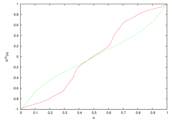
Figure 1: ${\cal K}^{(s)}(\alpha)$ as a function of the normalized rank $\alpha$. Here ${\cal K}^{(s)}(\alpha)$ has been computed by averaging over all phase space, with $N=128$ and $T=0.4$. The two curves are for two distinct disorder samples.

For both samples, and in general for all samples we have analyzed, the curve varies smoothly between $-1$ and $1$. This implies that $\pi(X)$ is a very broad function, which takes values of order one in its whole support. That means that large random correlations show up in the mean field model with a high frequency, their distribution is essentially uniform, which is a stronger effect than might have been expected. In Fig. 2 we show the data for the distribution of correlations in two different samples at $N=2048$ (and, as before, $T=0.4$). The curves are slightly smoother, but they are not dramatically different from the case of the smaller, $N=128$ system. As a matter of fact, we believe that $\pi(X)$ is not self averaging.

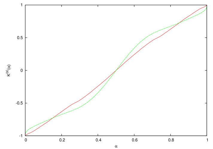
Figure 2: As in Fig. 1, but with $N=2048$.

A few comments about Fig. 1 and 2 are in order. As we have already said, the distribution of correlations is very broad, and its behavior is very different from an exponential decay: the correlations take all allowed values with very similar probabilities. The functional behavior is indeed very close to a linear one, but with sample to sample fluctuations that are clearly visible even at $N=2048$.

In this case the shape of the distribution of correlations is obviously determined by the presence of “many states”, and we have very clearly detected their manifestation here. When we inspect the whole phase space, the connected correlation functions coincide with the full correlation functions at all temperature, since, because of the ${\cal Z}_{2}$ symmetry of the Hamiltonian, all the magnetizations $m_{i}^{(s)}$ in sample $s$ are zero within errors (as mentioned before): we have verified that this is very well realized in our statistical sample.

A remarkable feature of Fig. 1 and 2 is the precise symmetry about the value ${\cal K}^{(s)}(\alpha)=0$. More remarkably, the deviations from the symmetry are much smaller than the disorder sample to disorder sample fluctuations. This is true with a very high degree of accuracy in all the disorder samples we have inspected. That such a symmetry must be present after averaging over the disorder is obvious, because of the gauge symmetry, involving both couplings and spins, of spin glasses [18, 19]. It is, however, unclear how symmetric a finite size sample should be. In the large $N$ limit the symmetry should hold for a typical system [22].

We have checked this symmetry property on small systems averaging over all spin configurations: we have enumerated all coupling configurations for $N=5$ and we have analyzed a number of coupling configurations for $N$ up to $21$. The symmetry clearly does not hold for the (quite atypical) ferromagnetic configuration, where all $J_{i,j}$ are equal to one. The symmetry is not exact even for balanced configurations (with the same number of positive and negative couplings), but for increasing $N$ these balanced configurations turn out indeed to be more and more symmetric already for small $N$ values, confirming our findings: the fact that a typical disorder configuration is, for $N\to\infty$, symmetric, manifests itself with great accuracy already for small $N$.

3.2 The correlation functions in one valley

We have discussed in the former paragraphs how correlation functions behave when thermally averaged over all phase space, i.e. allowing the system to visit all possible states. To better understand the slow decay (or, in other terms, the wide support of the probability density that we have observed), it is interesting to determine what happens when we constrain the dynamics to visit a single, given state only. As we have already explained, we do that (empirically) by running a local, slow dynamics, starting from spin configurations at thermal equilibrium.

We show in Fig. 3 ${\cal K}^{(s)}(\alpha)$ as a function of $\alpha$, for a system with $N=2048$ and low $T=0.4$, both as the result of integrating over all phase space and when it has been computed inside a given equilibrium free energy valley.

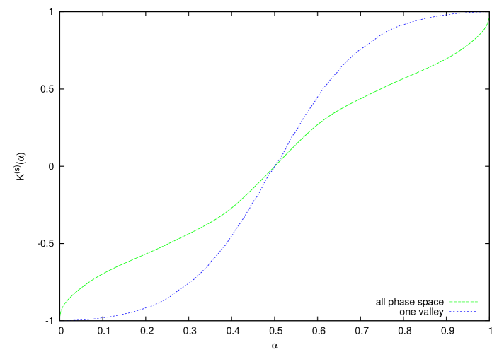
Figure 3: (color on line) ${\cal K}^{(s)}(\alpha)$ as a function of $\alpha$, for $N=2048$ and $T=0.4$. The curve that is higher in the left half of the plot is for ${\cal K}^{(s)}(\alpha)$ computed by averaging over all states (like in Fig. 2), while the curve that is higher in the right part of the plot is for correlation functions computed averaging over a single valley.

The situation depicted in Fig. 3 is typical of all samples with more than one valley (in samples where there is a single valley, i.e. that look paramagnetic, the two correlation functions are very similar). The single valley correlation functions are, in this typical situation, of the same shape as the complete ones, but the difference is obvious (a low value of $T$ is needed to observe it: we can only resolve this effect clearly at $T=0.4$, the lowest temperature value we analyze).

The one valley correlation, even when different from the complete correlation functions, have a finite support where their probability is significantly different from zero. They are always more biased toward $\pm 1$ than the complete function.

3.3 The connected correlation functions

The one valley correlation functions are indeed in at least one sense very different from the complete correlation functions: here the site dependent magnetizations $m_{i}$ are generically non zero (while when exploring the full phase space they are all zero). In this case the connected correlation functions ${\cal K}_{(c)\;ij}$ can be very different from the simple spin-spin function ${\cal K}_{ij}$. The question is how different they are? Since we are now exploring a single state, we would expect, far from criticality, a very localized distribution of the connected correlations and, looking at the correlations ordered by rank, a very fast, exponential decay.

We have computed these functions for a few samples, $N=2048$ and different temperature values, down to $T=0.4$. We plot in Fig. 4 both the full correlation function ${\cal K(\alpha)}$ and the connected correlation function ${\cal K}_{(c)}(\alpha)$ as a function of $\alpha$ for a single disorder sample.

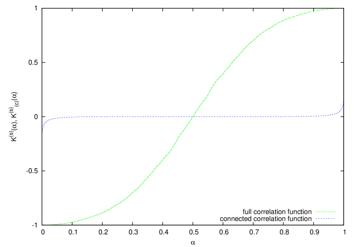
Figure 4: The full correlation function ${\cal K}(\alpha)$ and the connected correlation function ${\cal K}_{(c)}(\alpha)$ as a function of $\alpha$ for a single disorder sample.

Here the decay is clearly different from the former cases. The distribution function is indeed very localized, and the plot is surely indicative of an exponential decay of correlations.

4 Conclusions

As we argued in the Introduction, the very concept of complex systems as being “more than the sum of their parts” implies that they must possess long range correlations between their elements. Spin glasses, with their competing interactions and related complicated phase space structure, offered themselves as a natural laboratory to test this idea. In fact, the correlation functions in finite dimensional spin glasses, averaged over the random couplings, have long been known to be of long range, both from analytic and from numerical works. Here we argued that the individual samples must also display interesting long range correlation structures. As a very first step, we targeted the mean field model of spin glasses. This choice is motivated by the fact that the SK model is well understood, and while we are looking for an unusual, little investigated phenomenon, we are at least moving on familiar ground. Defined on the complete graph, the SK model does not have a concept of distance, which is an obvious drawback if we are to study long range correlations. However, as the correlations in the individual samples behave in a random, chaotic way even in finite dimensional spin glasses, the usual representation of correlation functions as functions of the distance is not very useful anyhow, and a good global characterization can be obtained by sorting all the $N(N-1)/2$ correlation coefficients according to magnitude, that is constructing the probability distribution of correlations. This construction can be taken over to the mean field model, and this was the object we have studied here under various conditions. The long range character of correlations was expected to manifest itself in the broadening of the distribution of correlations as we go into the ordered phase. We found that the effect is strikingly strong: when sampling the whole phase space the distribution of correlations turned out to be essentially uniform at low temperatures, that is any value between -1 and +1 appeared with basically the same probability, modulo small scale sample to sample fluctuations. While the other features we studied (size dependence, temperature dependence, connected versus full correlations, whole phase space versus individual valleys) worked out as expected on the basis of the many valleys picture, the extremely broad distribution of correlations is a surprise and this result stands out as the central message of this paper. It is an extra bonus that the second moment of this distribution turns out to be the same as the second moment of the overlap distribution, so the broadening of the distribution of correlations also signals the onset of the splitting of phase space into many pure states. Preliminary investigation [24] of spin glass correlations in other topologies (low dimensional Euclidean lattices and other graphs) indicates that a definite broadening of the probability density of correlations (albeit weaker than in the mean field case) is present also in these systems, that lends support to the conjecture that long range correlations are a general feature of many, perhaps all, complex systems. We intend to return to the problem of long range spin glass correlations in finite dimensions in a subsequent publication.

References

References

- [1] M. Mézard, G. Parisi and M. Virasoro, Spin Glass Theory and Beyond (World Scientific, Singapore 1987).
- [2] D. Sherrington and S. Kirkpatrick, Phys. Rev. Lett. 35, 1792 (1975).
- [3] C. De Dominicis and I. Kondor, Phys. Rev. B 27, 606 (1983).
- [4] C. De Dominicis and I. Kondor, J. de Physique Lett. 45, L205 (1984).
- [5] C. De Dominicis and I. Kondor, J. de Physique Lett. 46, L1037 (1985).
- [6] I. Kondor and C. De Dominicis, Europhys. Lett. 2, 617 (1986).
- [7] T. Temesvári, I. Kondor and C. De Dominicis, J. Phys. A: Math. Gen. 21 L1145 (1988).
- [8] C. De Dominicis, I. Kondor and T. Temesvári, Beyond the Sherrington-Kirkpatrick model, in Spin glasses and random fields, edited by A.P. Young, World Scientific, Singapore, 119-160, 1998.
- [9] E. Marinari, G. Parisi, and J. Ruiz-Lorenzo, Phys. Rev. B 58, 14852 (1998); C. De Dominicis, I.Giardina, E. Marinari, O.C. Martin, and F. Zuliani, Phys. Rev. B 72, 014443 (2005); F. Belletti et al. (the Janus Collaboration) Phys. Rev. Lett. 101, 157201 (2008); J. Stat. Phys. 135, 1121 (2009); P. Contucci, C. Giardinà, C. Giberti, G. Parisi and C. Vernia, Phys. Rev. Lett. 103, 017201 (2009); R. Alvarez-Banos et al. (the Janus collaboration), J. Stat. Mech. P06026 (2010); Phys. Rev. Lett. 105, 177202 (2010).
- [10] D.S. Fisher and D. Huse, Phys. Rev. Lett. 56, 1601 (1986); Phys. Rev. B 38, 386 (1988); A.J. Bray and M.A. Moore in Proceedings of the Heidelberg Colloquium on Glassy Dynamics (Lecture Notes in Physics 275), edited by J.L. van Hemmen and I. Morgenstern (Springer, Heidelberg, 1986).
- [11] J. Sinova, G. Canright, and A. H. MacDonald, Phys. Rev. Lett. 85, 2609 (2000).
- [12] J. Sinova, G. Canright, H. E. Castillo, and A. H. MacDonald, Phys. Rev. B 63, 104427 (2001).
- [13] K. Hukushima and Y. Iba, preprint cond-mat/0207123 (July 2002).
- [14] L. Correale, E. Marinari, and V. Martin-Mayor, Phys. Rev. B 66, 174406 (2002).
- [15] I. Kondor, Correlations in Complex Systems, invited talk at the International Workshop on Challenges and Visions in the Social Sciences, ETH Zurich, August 18-23, 2008; Strong Random Correlations in Complex Systems, invited talk at the 4th European PhD Complexity School, The Hebrew University, Jerusalem, September 10-14, 2008.
- [16] C.M. Newman and D.L. Stein, Phys. Rev. B 46, 973 (1992); A. Billoire and E. Marinari, Europhys. Lett. 60, 775 (2002); J. Lukic, E. Marinari, O. C. Martin and S. Sabatini, J. Stat. Mech. L10001 (2006).
- [17] N. Aral and A.N. Berker, Phys. Rev. B 79, 014434 (2009).
- [18] G. Toulouse, Commun. Phys. (London) 2, 115 (1977).
- [19] E. Marinari, C. Parrinello and R. Ricci, Nucl. Phys. B 362, 487 (1991).
- [20] K. Hukushima and K. Nemoto, J. Phys. Soc. Japan 65, 1604 (1996); M.C. Tesi, E.J. Janse van Rensburg, E. Orlandini and S.G. Whittington, J. Stat. Phys. 82, 155 (1996).
- [21] E. Marinari, Optimized Monte Carlo Methods in Advances in Computer Simulation, edited by J.Kertesz and I. Kondor, Springer-Verlag (1997).
- [22] B. Derrida, private communication.
- [23] A. Billoire and E. Marinari: J. Phys. A Math. Gen. 34, L727 (2001); A. Billoire, preprint arXiv:1003.6086 [cond-mat] (March 2010).
- [24] I. Kondor, I. Csabai and E. Mones, unpublished.