5-qubit Quantum error correction in a charge qubit quantum computer

Abstract

We implement the DiVincenzo-Shor 5 qubit quantum error correcting code into a solid-state quantum register. The quantum register is a multi charge-qubit system in a semiconductor environment, where the main sources of noise are phase decoherence and relaxation. We evaluate the decay of the density matrix for this multi-qubit system and perform regular quantum error corrections. The performance of the error correction in this realistic system is found to yield an improvement of the fidelity. The fidelity can be maintained arbitrarily close to one by sufficiently increasing the frequency of error correction. This opens the door for arbitrarily long quantum computations.

I Introduction

The task of building a quantum computer, allowing for massive quantum parallelism Deu85 , long-lived quantum state superposition and entanglement, is one of the big challenge of twenty-first century physics. It requires precise maintenance and manipulation of quantum systems at a level far from anything that has ever been done before. Many criteria, nicely summarized by the DiVincenzo criteria Div00 , need to be satisfied in order to be able to harness the power of quantum physics to extract powerful information processing, and while most of these criteria have been satisfied to a reasonable level by some prospect for the implementation of a quantum information processing device NO08 , no such prospect has yet been able to fulfill to a sufficient level all of these criteria at once. In particular, one criterion that not many prospects seem to be able to fulfill is that of scalability, the ability of the model to remain coherent for quantum systems with a large number of qubits.

Solid-state quantum registers seem to emerge as a medium that would allow for such scalability, while still being able to satisfy the other criteria NO08 . However, as for any physical implementation of quantum computing, it suffers from noise, dissipation processes mainly in the form of decoherence and relaxation Wei08 . To be able to use the power of quantum computation, we must be able to eliminate this noise and maintain quantum information throughout the processing. A general framework for doing so is quantum error correction (QEC) Shor95 ; Stea96 . It is known that by encoding a single logical qubit on sufficiently many physical qubits, we can correct arbitrary errors on a single physical qubit Shor95 . But what happens with more realistic multi-qubit errors?

In order to perform a quantum error correction, additional qubits are needed. However, these additional qubits can lead to a much higher rate of decoherence (even superdecoherence) superdcoh ; IHD05 . The implementation of the three-qubit repetition code has already been simulated for a cavity-QED setup OV10 , showing a significant but limited improvement for the preservation of quantum information. Here, we consider a realistic noise model for $N$ charge qubit quantum registers IHD05 , and simulate this noise model on encoded qubits to evaluate the efficiency of a QEC scheme. The quantum error correcting code (QECC) used is the 5 qubit DiVincenzo-Shor code DS96 .

We structure this work as follows: we first describe the representation for quantum systems we will be using, as well as that for the noise model. We then further analyze the physical model we study, and review the QECC we implement within this model. Section VI then contains the core of this work, that is, a description of the algorithm used for the simulation, followed by a discussion of the results obtained.

II Representation of quantum systems

We will be considering the basic unit of quantum information: the qubit. A qubit can be implemented by any two level quantum system, and so can be represented by a unit length vector in a two-dimensional complex Hilbert space, up to an equivalence relation for global phase. If we consider some prefered orthonormal basis states $\mathop{\left|0\right>}\nolimits$ and $\mathop{\left|1\right>}\nolimits$, a single qubit can be parametrized by 2 parameters $\theta\in[0,\pi]$ and $\phi\in[0,2\pi)$:

$$\mathop{\left|\psi\right>}\nolimits=\cos\left(\frac{\theta}{2}\right)\mathop{\left|0\right>}\nolimits+e^{i\phi}\sin\left(\frac{\theta}{2}\right)\mathop{\left|1\right>}\nolimits.$$ (II.1)

This is the Bloch sphere representation, for pure qubit systems.

When considering multiple interacting qubit systems, the overall system is described by the tensor product of the component Hilbert spaces. In general, once two systems have interacted, a complete description of the whole system cannot be obtained by a description of each subsystem: this is entanglement. Much of the power of quantum information processing comes from entanglement, it is a uniquely quantum resource. Note that this is also related to the difficulty of simulating a multi qubit quantum system: as a $N$ qubit quantum system cannot be completely described by each of the $N$ two dimensional subsystems, it must be described by a $2^{N}$ dimensional system, so that the memory required to store the information about a $N$ qubit quantum system scales exponentially with $N$, and so do the time required to simulate operations on this system.

This also raises the question of the description of subsystems of entangled systems. It turns out that the density operator formalism NC00 can solve this issue. In this formalism, a state $\psi$ is represented by a density matrix $\rho_{\psi}=|\psi\rangle\!\langle\psi|$ instead of by a state vector $\mathop{\left|\psi\right>}\nolimits$. Then, if we are only interested in subsequent evolution of a particular subsystem of the state $\psi$, we can do a partial trace NC00 over the other irrelevant subsytems and only evolve the reduced density matrix of the subsystem of interest. In this way, we obtain the right outcome statistic on this subsystem while not having to evolve a high-dimensionality state as required to describe the whole system completely. This density operator formalism also comes in handy for the description of statistical ensembles $\{p_{i},\mathop{\left|\psi_{i}\right>}\nolimits\}$, where the system is prepared in the state $\mathop{\left|\psi_{i}\right>}\nolimits$ with probability $p_{i}$. The corresponding density operator is $\rho=\sum_{i}p_{i}|\psi_{i}\rangle\!\langle\psi_{i}|$, and here also the evolution of this state leads to the right measurement statistics.

A closely related subject is that of quantum noise. As a quantum system cannot ever be completely isolated from its environment, they interact and then become entangled. So, even though the global system-environment pair undergoes unitary evolution, the main system does not, and this generates quantum noise. This is well described by the quantum operation formalism NC00 . Two types of noise in which we will be mostly interested will be decoherence and relaxation, and we will see that these are closely related to generalized dephasing channels DS05 and amplitude damping channels respectively GF05 ; NC00 .

Since the quantum system of interest will be subject to noise, we want a way to quantitatively describe how close it will remain to the initial quantum information we wished to preserve. A good measure of this is the fidelity Sch96 ; NC00 , and for a pure input state $\mathop{\left|\psi\right>}\nolimits$ evolving to a mixed state $\rho$, the fidelity is given by

$$F(\mathop{\left|\psi\right>}\nolimits,\rho)=\sqrt{\mathop{\left<\psi\,\right|}\nolimits\rho\mathop{\left|\psi\right>}\nolimits}.$$ (II.2)

III Quantum noise

The two main types of noise in which we will be interested are decoherence, which correspond to a loss of quantum coherence without loss of energy, and relaxation, which correspond to a loss of energy. We will see that these types of noise are closely related to well-studied channels: generalized dephasing channels DS05 ; BHTW10 and amplitude damping channels GF05 ; NC00

III.1 Generalized dephasing channels

Generalized dephasing channels correspond to physical processes in which there is loss of quantum coherence without loss of energy. That is, there exist a preferred basis, called the dephasing basis, such that pure states in that basis are transmitted without error, but pure superposition get mixed, and quantum information is lost to the environment.

If we let $A$ be the input system with orthonormal basis $\{\mathop{\left|i\right>}\nolimits^{A}\}$, $B$ be the output system with orthonormal basis $\{\mathop{\left|i\right>}\nolimits^{B}\}$, and $E$ be the environment with normalized, not necessarily orthogonal states $\{\mathop{\left|\xi_{i}\right>}\nolimits^{E}\}$, then an isometric map from the input system to the output-environment system is given by

$$U^{A\rightarrow BE}=\sum_{i}\mathop{\left|i\right>}\nolimits^{B}\mathop{\left|\xi_{i}\right>}\nolimits^{E}\mathop{\left<i\,\right|}\nolimits^{A}.$$ (III.1)

Then, starting with an input state $\rho^{A}$, we get the output state $\sigma^{B}$ by first applying the isometry $U^{A\rightarrow BE}$, then tracing over $E$:

$$\sigma^{B}=\mathop{{\mathrm{Tr}}_{E}}(U\rho^{A}U^{\dagger})=\sum_{i,j}\mathop{\left<i\,\right|}\nolimits\rho^{A}\mathop{\left|j\right>}\nolimits|i\rangle\!\langle j|^{B}\langle\xi_{j}|\xi_{i}\rangle.$$ (III.2)

As we can see, in this representation, the output corresponds to the Hadamard product between the $(\mathop{\left<i\,\right|}\nolimits\rho^{A}\mathop{\left|j\right>}\nolimits)$ input matrix and the $(\langle\xi_{i}|\xi_{j}\rangle^{\dagger})$ decoherence matrix. Also, since the ${\mathop{\left|\xi_{i}\right>}\nolimits}$ are normalized, $\langle\xi_{i}|\xi_{i}\rangle=1$, the diagonal terms are left unchanged:

$$\mathop{\left<i\,\right|}\nolimits\sigma^{B}\mathop{\left|i\right>}\nolimits=\mathop{\left<i\,\right|}\nolimits\rho^{A}\mathop{\left|i\right>}\nolimits.$$ (III.3)

These diagonal terms correspond to the probability of measuring the quantum state in the corresponding dephasing basis state, while the off-diagonal terms are coherence (phase) terms. For these off-diagonal terms, the Cauchy-Schwarz inequality ($|\langle\xi_{i}|\xi_{j}\rangle|^{2}\leq\langle\xi_{i}|\xi_{i}\rangle\langle\xi_{j}|\xi_{j}\rangle=1$) tells us that the output terms must be smaller than or equal to the input terms: $|\mathop{\left<i\,\right|}\nolimits\sigma^{B}\mathop{\left|j\right>}\nolimits|\leq|\mathop{\left<i\,\right|}\nolimits\rho^{A}\mathop{\left|j\right>}\nolimits|$. In the special case where the $\{\mathop{\left|\xi_{i}\right>}\nolimits^{E}\}$ are also orthogonal, we obtain a completely dephasing channel, which kills all off-diagonal terms, $\mathop{\left<i\,\right|}\nolimits\sigma^{B}\mathop{\left|j\right>}\nolimits=0$ if $i\neq j$. For a subsequent measurement in the dephasing basis, this yields a classical statistical output with no quantum coherence terms: $\sigma^{B}=\sum_{i}\mathop{\left<i\,\right|}\nolimits\rho^{A}\mathop{\left|i\right>}\nolimits|i\rangle\!\langle i|^{B}$.

III.2 Amplitude damping channels

Amplitude damping channels correspond to physical processes in which there is a loss of energy from the quantum system of interest to the environment. That is, there is a probability that a quantum state passes from a higher energy excited state to a lower energy state. For the two-dimensional quantum systems in which we are mostly interested, this corresponds to a probability of passing from the excited state to the ground state, while the ground state is left unaffected. In the quantum operation formalism, this channel has operation elements $\{E_{0},E_{1}\}$:

$$E_{0}=\left(\begin{array}[]{cc}1&0\\ 0&\sqrt{1-\gamma}\end{array}\right),E_{1}=\left(\begin{array}[]{cc}0&\sqrt{\gamma}\\ 0&0\end{array}\right),$$ (III.4)

where the matrix representation is given in the energy eigenbasis, and the parameter $\gamma$ corresponds to the probability of decay. Then, for some input state $\rho^{A}$, we get an output state $\sigma^{B}$:

$$\sigma^{B}=\sum_{i=0,1}E_{i}\rho^{A}E_{i}^{\dagger}.$$ (III.5)

If we represent the action of the channel as $\mathcal{E}$, i.e. $\mathcal{E}(\rho^{A})=\sigma^{B}$, we can extend this definition to multi-qubit systems. Making the assumption that energy lost for each two-dimensional subsystem is independent, a tensor product of this channel, $\mathcal{E}^{\otimes n}$, corresponds to a loss of energy in each subsystem independently.

IV Decoherence and relaxation in charge qubit registers

Solid state quantum systems represent an interesting prospect for the physical implementation of scalable quantum devices NO08 . A lot of research goes into implementation of superconducting qubits MSS01 ; WS05 . Another important avenue of research are quantum dots, in which two level quantum systems can be implemented in either the spin or position degree of freedom of the electron trapped in the dots. While spin quantum dots have a longer decoherence time Elz04 ; Pet06 , spins are also more difficult to manipulate. In charge quantum dots, where the basis states correspond to the position of the electron in either of two adjacent quantum dots, the coupling is strong and hence fast manipulation is possible, but this also leads to shorter decoherence times. We will consider such a system, which offers an interesting playground for current technology research Sh07 ; Hay03 . Moreover, the decoherence for $N$ qubit quantum registers, which can be seen in FIG. 1, has already been computed by Ischii et al. IHD05 , and it is this model which is used in this simulation.

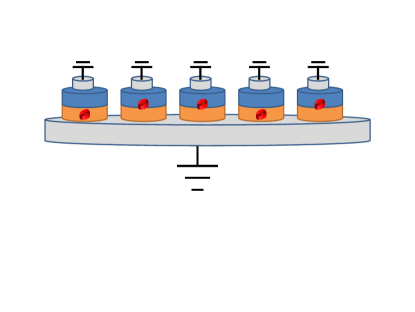
Figure 1: Physical model for the 5-qubit quantum register. The qubit geometry is inspired from recent experiments on coherent level mixing in vertical quantum dots Chris .

It is found that for these charge quantum dots, the decoherence of the quantum system can be represented as a generalized dephasing channel in the canonical basis of the charge qubits, corresponding to the position eigenstates. Indeed, pure states in that basis are perfectly transmitted, while pure superpositions become noisy. It is then possible to compute the evolution of the quantum register by taking the Hadamard product of the input density matrix with a decoherence matrix computed in IHD05 , thus getting the decohered output state. We chose as physical timescale unit $\omega_{0}$, which corresponds to the upper cut-off frequency. In charge qubits in GaAs we typically have

$$\omega_{0}=0.2\times 10^{-10}s.$$ (IV.1)

This leads to the decay of the off-diagonal elements of the N-qubit density matrix. The structure of this decay is non-trivial and is shown in FIG. 2. In general, this leads to an error, which cannot be reduced to a single qubit error.

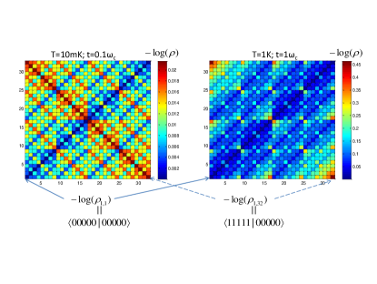
Figure 2: (Color online) Matrix elements of the decay function density matrix due to decoherence.

In addition, this decoherence model does not take into account any relaxation the system might be subject to. We assume that the relaxation is independent of decoherence, and also that energy loss for each qubit is independent. For each two dimensional quantum subsystem, if $\mathop{\left|0\right>}\nolimits$ and $\mathop{\left|1\right>}\nolimits$ correspond to the two position eigenstates, then the two energy eigenstates are $\mathop{\left|+\right>}\nolimits=\frac{1}{\sqrt{2}}(\mathop{\left|0\right>}\nolimits+\mathop{\left|1\right>}\nolimits)$ for the ground state, and $\mathop{\left|-\right>}\nolimits=\frac{1}{\sqrt{2}}(\mathop{\left|0\right>}\nolimits-\mathop{\left|1\right>}\nolimits)$ for the excited state. We can then compute the effect of relaxation by operating a tensor product of amplitude damping channels to each qubit in the register, where the operation elements (III.4) are in the $\{\mathop{\left|+\right>}\nolimits,\mathop{\left|-\right>}\nolimits\}$ basis. The decay parameter $\gamma$ is time $(t)$ and temperature $(T)$ dependent,

$$\gamma=1-exp(-t\cdot T),$$ (IV.2)

setting $k_{B}=\hbar=1$.

V Quantum error correction with a perfect 5 qubit code

Since our quantum register is subject to noise, we want to encode an input quantum state in such a way that we can preserve the quantum information even when the physical system undergoes noise. A general framework for doing this is quantum error correction (QEC) Shor95 ; Stea96 , which encode a logical qubit containing the quantum information on multiple physical qubits, and then usually by performing syndrome measurements on these physical qubits, we can determine a certain set of errors, and apply the corresponding correction NC00 . Many quantum error correcting codes (QECC) have been found that can correct an arbitrary error on a single physical qubit, and it is known that the smallest such codes require 5 physical qubits LMPZ96 .

One of these 5 qubit codes is the DiVincenzo-Shor QECC DS96 . The code words for the logical states $\{\mathop{\left|0\right>}\nolimits_{L},\mathop{\left|1\right>}\nolimits_{L}\}$ are NO08 :

$$\mathop{\left|0\right>}\nolimits_{L} = \frac{1}{4}\big{(}\mathop{\left|00000\right>}\nolimits+\mathop{\left|11000\right>}\nolimits+\mathop{\left|01100\right>}\nolimits+\mathop{\left|00110\right>}\nolimits$$

$$+ \mathop{\left|00011\right>}\nolimits+\mathop{\left|10001\right>}\nolimits-\mathop{\left|10100\right>}\nolimits-\mathop{\left|01010\right>}\nolimits$$

$$- \mathop{\left|00101\right>}\nolimits-\mathop{\left|10010\right>}\nolimits-\mathop{\left|01001\right>}\nolimits-\mathop{\left|11110\right>}\nolimits$$

$$- \mathop{\left|01111\right>}\nolimits-\mathop{\left|10111\right>}\nolimits-\mathop{\left|11011\right>}\nolimits-\mathop{\left|11101\right>}\nolimits\big{)}$$

$$\mathop{\left|1\right>}\nolimits_{L} = \frac{1}{4}\big{(}\mathop{\left|11111\right>}\nolimits+\mathop{\left|00111\right>}\nolimits+\mathop{\left|10011\right>}\nolimits+\mathop{\left|11001\right>}\nolimits$$

$$+ \mathop{\left|11100\right>}\nolimits+\mathop{\left|01110\right>}\nolimits-\mathop{\left|01011\right>}\nolimits-\mathop{\left|10101\right>}\nolimits$$

$$- \mathop{\left|11010\right>}\nolimits-\mathop{\left|01101\right>}\nolimits-\mathop{\left|10110\right>}\nolimits-\mathop{\left|00001\right>}\nolimits$$

$$- \mathop{\left|10000\right>}\nolimits-\mathop{\left|01000\right>}\nolimits-\mathop{\left|00100\right>}\nolimits-\mathop{\left|00010\right>}\nolimits\big{)}$$

with stabilizers Gott96 :

$$M_{0}=I\otimes Z\otimes X\otimes X\otimes Z$$

$$M_{1}=Z\otimes I\otimes Z\otimes X\otimes X$$

$$M_{2}=X\otimes Z\otimes I\otimes Z\otimes X$$ (V.1)

$$M_{3}=X\otimes X\otimes Z\otimes I\otimes Z,$$

which leave the code invariant. The $X$ and $Z$ operators are respectively the $X$ and $Z$ Pauli operators. The encoding circuit can be seen in NO08 . This is a perfect non-degenerate code, meaning that all single qubit errors map to a different syndrome, as can be seen in TABLE 1. To obtain a measurement of the error syndrome, we measure observables in the eigenbasis of each of the four stabilizers in (V), and depending on the outcome of these four measurements we apply the corresponding correction from TABLE 1.

An alternative to these multi-qubit measurements NC00 is to use ancillary qubits to conditionnally apply each of the four stabilizers on a $\mathop{\left|+\right>}\nolimits$ state, thus recording the phase (M0-M3 have eigenvalues $\pm 1$). Measuring these four ancilla qubits in the $\{\mathop{\left|+\right>}\nolimits,\mathop{\left|-\right>}\nolimits\}$ basis then gives the same result as above without having to perform multi-qubit measurements. This syndrome measurement circuit is given in NO08 .

$M$	0	1	2	3	4	5	6	7	8	9	10	11	12	13	14	15
$E_{M}$	$I$	$Z_{2}$	$X_{0}$	$Z_{3}$	$X_{3}$	$X_{1}$	$Z_{4}$	$Y_{3}$	$Z_{1}$	$X_{4}$	$X_{2}$	$Y_{2}$	$Z_{0}$	$Y_{1}$	$Y_{0}$	$Y_{4}$

Table 1: Table of the different possible single qubit errors $E_{M}$, with their associated syndrome measurement output $M$, which has binary expension $M_{3}M_{2}M_{1}M_{0}$.

This code is guaranteed to correct any single qubit error, but it is not designed to correct multi-qubit errors, which our noise model will introduce. It will then be interesting to see how well this code will perform for an approximate correction of multi-qubit errors.

VI Quantum error correction in a charge qubit quantum computer

The qubit model for physical implementation we consider in this simulation is a charge quantum dot. The two principal sources of noise with this model are decoherence and relaxation.

The effect of decoherence on a $N$-qubit register had been computed in IHD05 , where decoherence is caracteristic of a generalized dephasing channel DS05 , leaving computational basis states unaffected.

The effect of relaxation correspond to a probabilistic loss of energy, where the excited state correspond to the $\mathop{\left|-\right>}\nolimits$ state, and the ground state correspond to the $\mathop{\left|+\right>}\nolimits$ state. We make the assumption that this relaxation for each qubit is independant, so that we implement this noise has a tensor product of an amplitude damping channel in the $\{\mathop{\left|+\right>}\nolimits,\mathop{\left|-\right>}\nolimits\}$ basis, on each qubit.

To counter the effect of noise, we encode a logical qubit into 5 qubits, using the DiVincenzo-Shor QECC, which can perfectly correct errors on a single qubit. However, the noise model used creates errors on multiple qubits, and so it is not obvious that QEC with the DiVincenzo-Shor code can extend the lifetime of our logical qubit.

Here, we verify the effect of such a quantum error correction scheme, for different input states and different frequencies of correction. The algorithm used for the simulation is presented first, and the results of the simulation are presented next.

VI.1 Implementation of QEC algorithm

An overview of the algorithm can be seen in FIG. 3. First, the logical qubit is encoded into 5 physical qubits using the DiVincenzo-Shor QECC. This encoding is assumed to be perfect. We only consider pure input qubits, which are completely caracterized by two real parameters corresponding to their position on the Bloch sphere: $\theta\in[0,\pi]$, $\phi\in[0,2\pi)$.

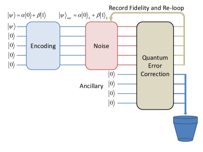
Figure 3: Overview of the algorithm for the simulation of quantum error correction of a solid-state quantum register.

After encoding, the quantum register is subjected to noise for a given period of time $t$, depending on the frequency of error correction. In our simulation, the decoherence noise and the relaxation noise are applied successively, and we checked numerically that the order does not affect the result. The intensity of the noise depends on the temperature $T$ of simulation, and the probability of relaxation is adjusted such that without error correction, after a time $\omega_{0}$ the fidelity of the noisy state with respect to the pure input state is the same as that of decoherence.

Quantum error correction is then performed. Here we assume perfect operation of each component of the QEC algorithm. However, instead of performing the measurement of the syndrome and then applying the corresponding correction (see TABLE 1), we defer the measurement to the end of the circuit and perform conditional quantum correction NC00 ; NO08 . To do so, four ancillary qubits are used to record the syndrome measurements. It is possible to avoid multi-qubit measurements by using these ancillary qubits, but the drawback is that we pass from a 5 qubit quantum system to a 9 qubit quantum system. This increases the difficulty of physical implementation because of the additionnal qubits, and also because every round of QEC requires four fresh ancilla qubits. This also slows the simulation a lot, since we pass from a $2^{5}=32$ dimensional complex vector space to a $2^{9}=512$ one, and the matrix operations are accordingly scaled.

After performing the conditional QEC, these ancilla qubits are traced over, which corresponds to a measurement without a record of the outcome. This gives an output state which is a statistical ensemble corresponding to the different possible corrected states.

To perform the conditional quantum error correction, we implement a quantum circuit which would correct for the different errors in TABLE 1, corresponding to the value of the ancilla qubits. If we let $\mathop{\left|M\right>}\nolimits$ correspond to the ancilla state with binary expansion $M_{3}M_{2}M_{1}M_{0}$, for $M$ running from $0$ to $15$, and if $E_{M}$ is the corresponding error, then the QEC circuit is

$$\prod_{M=0}^{15}\big{(}E_{M}^{\dagger}\otimes|M\rangle\!\langle M|+I_{5}\otimes(I_{4}-|M\rangle\!\langle M|)\big{)},$$ (VI.1)

where the order in the operator product is irrelevant since the terms commute.

Following the quantum error correction step, a record of the fidelity of this output state compared to the input state is taken. We then reloop over the noise, quantum error correction and fidelity recording steps, until the sum of all the noise time steps add up to the desired total time of the simulation.

VI.2 QEC performance

VI.2.1 Decoherence

We can see on FIG. 4 the results of the simulation when our quantum register is subject only to decoherence. With a small frequency of error correction of $\omega_{0}^{-1}$, the fidelity is already improved over the uncorrected qubit. For a basis qubit, either $\mathop{\left|0\right>}\nolimits$ or $\mathop{\left|1\right>}\nolimits$, we do not have decoherence, but the encoded state does suffer from decoherence. The encoded basis states however do exhibit an interesting behavior when they are decohered, but not error corrected. In fact, even though the noise takes the 5 qubit state out of the code, when decoded we still get back the original basis state. For these basis states, we could understand this behavior by noting that the code words for the logical $\mathop{\left|0\right>}\nolimits$ and $\mathop{\left|1\right>}\nolimits$ contain different 5 qubit basis states, as we can see in (V). But for pure superposition of these basis states, if we do not error correct the encoded states, it also decoheres in a way such that once decoded, the same state as the unencoded decohered state is obtained, which is even more surprising.

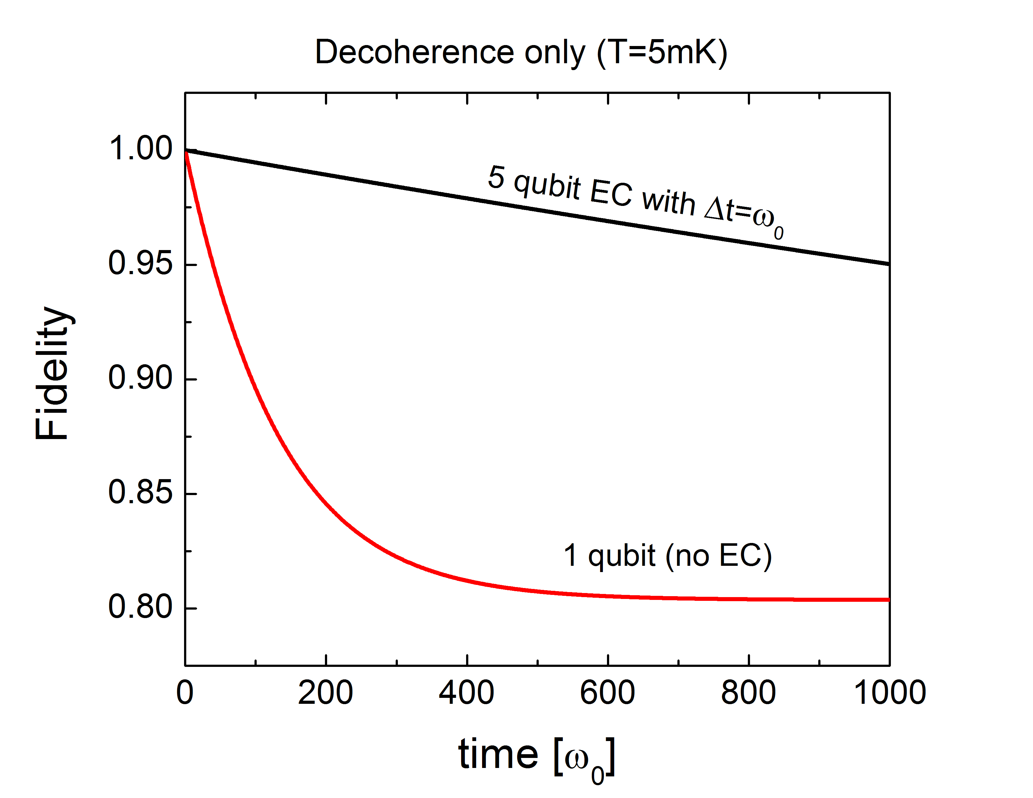
Figure 4: Simulation of quantum error correction with only decoherence. The time between two successive QECs is $\Delta t=\omega_{0}$. For a total of $1000\omega_{0}$, the top curve shows the result of the QEC and the non-corrected 1qubit decoherence is shown in the bottom curve. The input qubit is $\mathop{\left|\psi\right>}\nolimits=\cos\left(\frac{1}{2}\right)\mathop{\left|0\right>}\nolimits+e^{i}\sin\left(\frac{1}{2}\right)\mathop{\left|1\right>}\nolimits$ and the temperature is assumed to be 5 mK.

VI.2.2 Relaxation

We can see in FIG. 5 the results of the simulation when we only consider relaxation affecting our quantum register. This type of noise has a stronger temperature dependency and is stronger than decoherence for temperatures above 5 mK, at which point we obtain on average a similar drop in fidelity at 1 $\omega_{0}$. It is also harder to correct than decoherence. We thus need a much higher frequency of quantum error correction to keep the fidelity close to 1 until we have reached a saturation in relaxation, that is we have reached the lowest energy state for the unencoded qubit. This low energy state is the only state invariant under action of the channel.

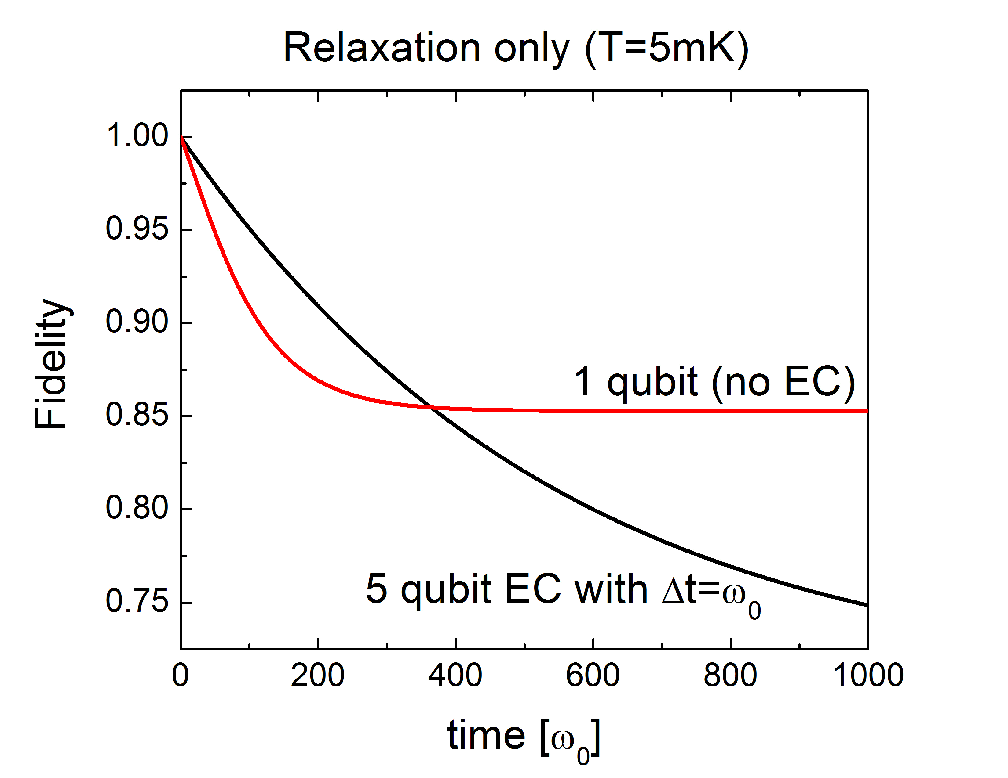
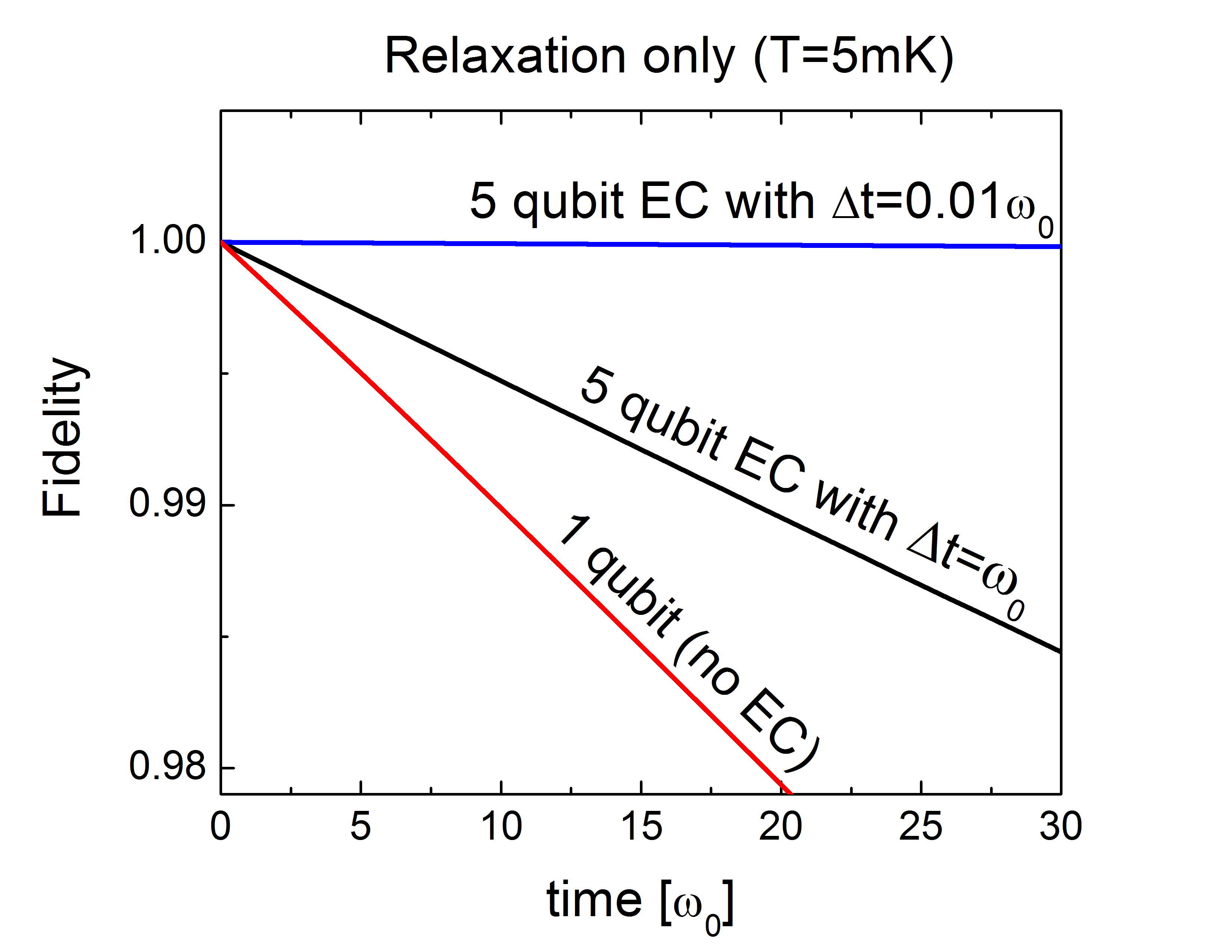
Figure 5: Simulation of quantum error correction with only relaxation: In the left graph the fidelity as a function of time is shown for the same $\Delta t=\omega_{0}$ as in FIG. 4. By reducing the time interval between two QECs the fidelity remains close to one as seen in the right graph. For both graphs, the input qubit is the same as in FIG. 4.

VI.2.3 Simultaneous decoherence and relaxation

When combining the effect of decoherence and relaxation, the frequency of error correction is on the order of what is needed for relaxation, since relaxation is much harder to correct than decoherence. Here too, when taking into account decoherence and relaxation, we are still able to maintain the fidelity arbitrarily close to one (see FIG. 6). This tells us that even though it may require a high frequency of quantum error correction, the 5 qubit code is able to correct a realistic multi-qubit error system.

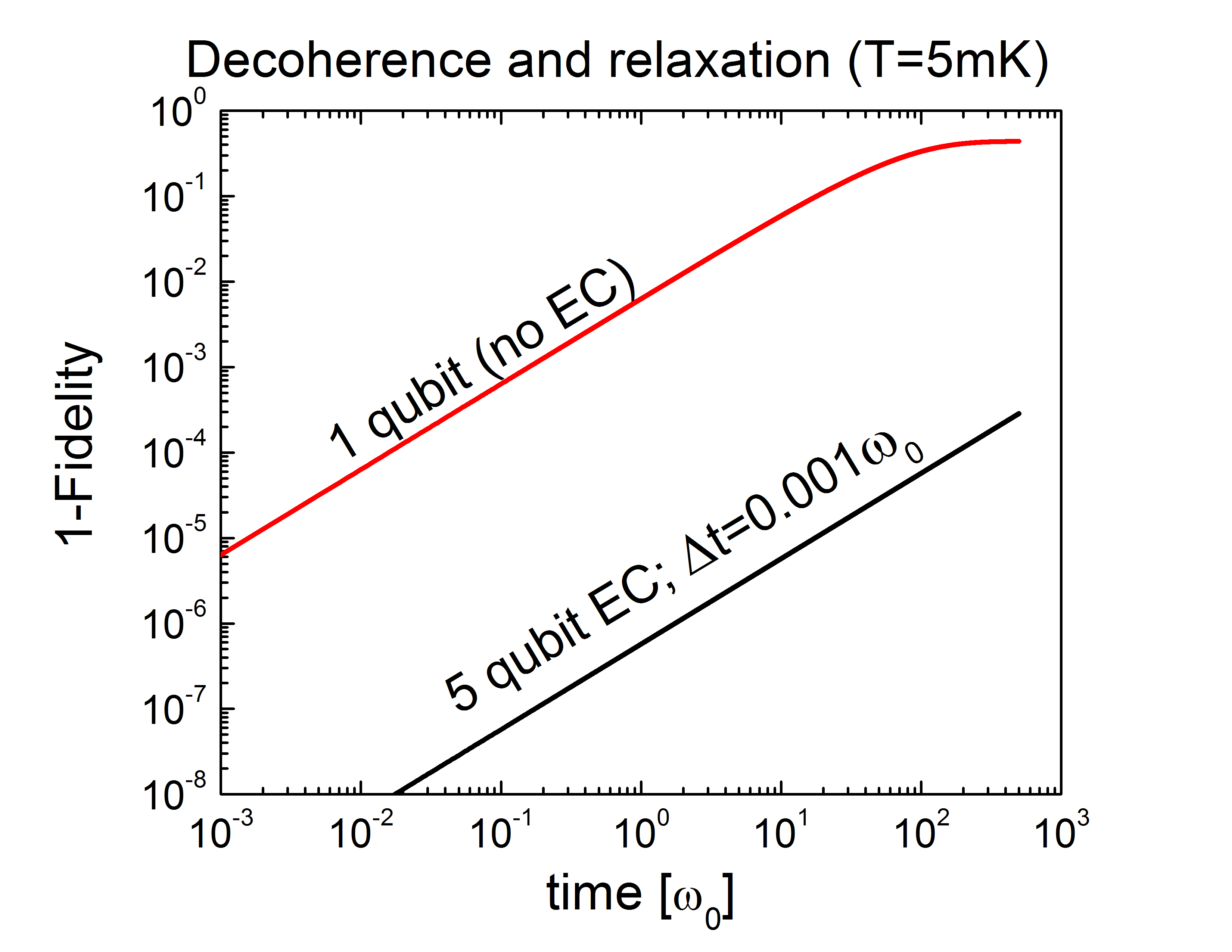
Figure 6: 1 minus fidelity is shown as a function of time for a very short $\Delta t=0.001\omega_{0}$. The high-frequency QEC for joint decoherence and relaxation enables the quantum information to be preserved almost perfectly. The input qubit is the same as in FIG. 4.

VI.3 Discussion

We have only considered noise in the N-qubit system. That is, an important assumption made for our simulation is that of a perfect operation of the QEC algorithm. However, in a realistic fault-tolerant quantum computation (FTQC) Shor96 , errors will also occur within the operation of the gates and measurements, and this also during the QEC steps. Similar concerns led some physicists to wonder if the error model adopted to get to the threshold theorem KL96 ; AB96 for FTQC is physical enough so that FTQC is possible at all Dya06 . Hence, such a simulation, with a realistic model for operations, would be an important step toward determining if physical implementations of quantum computers are possible. It is possible that these types of errors can be corrected in a similar manner, but this is beyond the scope of this work.

The model considered introduces multi-qubit errors, which are much smaller than full single-qubit ones when the time evolution is very short. At the lowest order, we showed that these small multi-qubit errors can be corrected by single-qubit QEC codes. However, this increases the required QEC frequency, but it is certainly possible to find other error correcting schemes optimized for multi-qubit errors, which would require a lower QEC frequency.

Also, since the decoherence time for charge qubits is short, the frequency of QEC required to maintain good fidelity for extended periods is too high to be feasible experimentally with current techniques. However, this is a proof of principle and it is reasonable to expect that for other implementations of qubits like spin qubits or superconducting qubits, where decoherence times can be much longer, similar performances would require a QEC frequency that is attainable experimentally.

VII Conclusion

We have simulated the implementation of the 5 qubit DiVincenzo-Shor QECC for a charge qubit quantum register. The register was subjected to a realistic noise model, consisting of decoherence and relaxation. Even though the QECC is designed to perfectly correct only single qubit errors, an application of the QEC routine with a high enough frequency was able to limit the effect of multi-qubit errors introduced by our noise model. In fact, by adjusting the frequency of error correction, we can get the fidelity as close to one as possible, and for extended periods of time. When considering both types of noise separately, relaxation showed to be harder to error correct than decoherence, requiring higher frequency of QEC for the same results.

References

- (1) D. Deutsch, Quantum theory, the Church-Turing principle and the universal quantum computer, Proc. R. Soc. Lond. A, 400:97 (1985).
- (2) D. P. DiVincenzo, The Physical Implementation of Quantum Computation, Fortschr. Phys. 48, 771 (2000). arXiv:quant-ph/0002077v3
- (3) M. Nakahara and T. Ohmi, Quantum Computing: From Linear Algebra to Physical Realizations, (CRC Press, 2008).
- (4) U. Weiss, Quantum dissipative systems, (World Scientific publishing co., third ed., 2008).
- (5) P. W. Shor, Scheme for reducing decoherence in quantum computer memory, Phys. Rev. A 52, 2493 (1995).
- (6) A. Steane, Simple Quantum Error Correcting Codes, Phys. Rev. A 54, 4741 (1996). arXiv:quant-ph/9605021v1
- (7) G. M. Palma, K. A. Suominen and A. K. Ekert, Quantum computers and dissipation, Proc. Roy. Soc. Lond. A 452, 567 (1996). arXiv:quant-ph/9702001v1
- (8) B. Ischi, M. Hilke and M. Dube, Decoherence in a N-qubit solid-state quantum register, Phys. Rev. B 71, 195325 (2005). arXiv:quant-ph/0411086v2
- (9) C. Ottaviani amd D. Vitali, Implementation of a three-qubit quantum error-correction code in a cavity-QED setup, Phys. Rev. A 82, 012319 (2010). arXiv:quant-ph/1005.3072v2
- (10) D. P. DiVincenzo and P. W. Shor, Fault-Tolerant Error Correction with Efficient Quantum Codes, Phys. Rev. Lett. 77, 3260 (1996). arXiv:quant-ph/9605031v2
- (11) M. A. Nielsen and I. L. Chuang, Quantum Computation and Quantum Information, (Cambridge Univ. Press, 2000).
- (12) I. Devetak and P. W. Shor, The capacity of a quantum channel for simultaneous transmission of classical and quantum information, Commun. Math. Phys. 256, 287 (2005) [ISI]. arXiv:quant-ph/0311131
- (13) V. Giovannetti and R. Fazio, Information-capacity description of spin-chain correlations, Phys. Rev. A 71, 032314 (2005). arXiv:quant-ph/0405110v3
- (14) B. W. Schumacher, Sending entanglement through noisy quantum channels, Phys. Rev. A 54, 2614 (1996). arXiv:quant-ph/9604023v1
- (15) Kamil Bradler, Patrick Hayden, Dave Touchette, and Mark M. Wilde, Trade-off capacities of the quantum Hadamard channels, Phys. Rev. A 81, 062312 (2010). arXiv:quant-ph/1001.1732v2
- (16) Y. Makhlin, G. Schon and A. Shnirman, Quantum-state engineering with Josephson-junction devices, Rev. Mod. Phys. 73, 357 (2001). arXiv:cond-mat/0011269v1
- (17) G. Wendin and V. S. Shumeiko, Superconducting Quantum Circuits, Qubits and Computing, Prepared for Handbook of Theoretical and Computational Nanotechnology (2005). arXiv:cond-mat/0508729v1
- (18) J. M. Elzerman, R. Hanson, L. H. Willems van Beveren, B. Witkamp, L. M. K. Vandersypen and L. P. Kouwenhoven, Single-shot read-out of an individual electron spin in a quantum dot, Nature 430, 431 (2004). arXiv:cond-mat/0411232v2
- (19) J.R. Petta, A.C. Johnson, J.M. Taylor, E.A. Laird, A. Yacoby, M.D. Lukin, C.M. Marcus, M.P. Hanson and A.C. Gossar, Preparing, manipulating, and measuring quantum states on a chip, Physica E 35, 251 (2006).
- (20) G. Shinkai, T. Hayashi, Y. Hirayama and T. Fujisawa, Controlled resonant tunneling in a coupled double-quantum-dot system, Appl. Phys. Lett. 90 103116 (2007).
- (21) T. Hayashi, T. Fujisawa, H. D. Cheong, Y. H. Jeong, and Y. Hirayama Coherent Manipulation of Electronic States in a Double Quantum Dot, Phys. Rev. Lett. 91, 226804 (2003). arXiv:cond-mat/0308362v1
- (22) C. Payette, S. Amaha, G. Yu, J. A. Gupta, D. G. Austing, S. V. Nair, B. Partoens, and S. Tarucha, Coherent level mixing in dot energy spectra measured by magnetoresonant tunneling spectroscopy of vertical quantum dot molecules, Phys. Rev. B 81, 245310 (2010).
- (23) R. Laflamme, C. Miquel, J. P. Paz and W. H. Zurek, Perfect quantum error correction code, Phys. Rev. Lett. 77, 198 (1996). arXiv:quant-ph/9602019v1
- (24) D. Gottesman, A Class of Quantum Error-Correcting Codes Saturating the Quantum Hamming Bound, Phys. Rev. A 54, 1862 (1996). arXiv:quant-ph/9604038v2
- (25) P. W. Shor, Fault-tolerant quantum computation, 37th Symposium on Foundations of Computing, IEEE Computer Society Press, 1996, pp. 56-65. arXiv:quant-ph/9605011v2
- (26) E. Knill, R. Laflamme, Concatenated Quantum Codes, arXiv:quant-ph/9608012v1.
- (27) D. Aharonov, M. Ben-Or, Fault Tolerant Quantum Computation with Constant Error, Proceedings of the 29th Annual ACM Symposium on Theory of Computing, 1997, pp. 176-188. arXiv:quant-ph/9611025v2
- (28) M. I. Dyakonov, Is Fault-Tolerant Quantum Computation Really Possible?, Future Trends in Microelectronics. Up the Nano Creek, Wiley (2007), pp. 4-18. arXiv:quant-ph/0610117v1