Abstract

We analyze the adjoint field inflation in supersymmetric (SUSY) $SU(5)$ model. In minimal SUSY $SU(5)$ hybrid inflation monopoles are produced at the end of inflation. We therefore explore the non-minimal model of inflation based on SUSY $SU(5)$, like shifted hybrid inflation, which provides a natural solution for the monopole problem. We find that the supergravity corrections with non-minimal Kähler potential are crucial to realize the central value of the scalar spectral index $n_{s}\simeq 0.96$ consistent with the seven year WMAP data. The tensor to scalar ratio $r$ is quite small, taking on values $r\lesssim 10^{-5}$. Due to $R$-symmetry massless $SU(3)$ octet and $SU(2)$ triplet supermultiplets are present and could spoil gauge coupling unification. To keep gauge coupling unification intact, light vector-like particles are added which are expected to be observed at LHC.

1 Introduction

Inflation is one of the most motivated scenarios for the early universe, which is consistent with the recent cosmological observations on the cosmic microwave background radiation and the large-scale structure in the universe. In order to construct a consistent model of inflation, an extension of the Standard Model (SM) is required. The supersymmetric (SUSY) grand unified theory (GUT) models provide a natural framework for hybrid inflation [1]-[11]. On the other hand, supersymmetric $SU(5)$ is the simplest extension of the SM which may realize hybrid inflation through the adjoint scalar field, which is responsible for breaking the $SU(5)$ gauge symmetry into SM gauge group $G_{SM}\equiv SU(3)_{c}\times SU(2)_{L}\times U(1)_{Y}$. However, in the standard minimal version of SUSY hybrid inflation the gauge symmetry is broken at the end of inflation, and topological defects are copiously formed. To overcome this problem, we consider the leading order non-renormalizable term in the superpotential of SUSY $SU(5)$ hybrid inflation. This class of inflationary models is known as shifted hybrid inflation, which have been introduced in Ref. [12] in the context of a supersymmetric Pati-Salam model. The inclusion of the non-renormalizable term introduces a non-trivial flat direction along which $SU(5)$ gauge symmetry is spontaneously broken through the appropriate Higgs fields acquiring non-zero vacuum expectation values (vevs). This direction then can be used as an inflationary trajectory with one-loop radiative corrections providing the necessary slope for slow-roll inflation. However, since $SU(5)$ is broken during inflation, one finds that for a certain range of parameters, the system always passes through the above mentioned inflationary trajectory before falling into the SUSY vacuum. Therefore, the magnetic monopole problem is solved for all initial conditions.

The scalar spectral index $n_{s}$ in shifted hybrid inflation, driven solely by radiative corrections, is typically of order $0.98$ with the number of e-foldings $N_{0}\simeq 53$ and lies outside the seven year Wilkinson Microwave Anisotropy Probe (WMAP7) 1-$\sigma$ bounds [13]. Including supergravity (sugra) corrections with minimal Kähler potential further enhances the scalar spectral index to exceed unity and a blue-tilted scalar spectral index is obtained as emphasized in Refs. [4, 14, 15, 16]. The non-minimal Kähler potential plays a crucial role in reducing $n_{s}$ and making it compatible with the WMAP7 data as shown in Refs. [17, 18, 19]. In SUSY $SU(5)$ shifted hybrid inflation we show that the central value of the scalar spectral index $n_{s}\simeq 0.96$ can be realized in the presence of a small negative mass term generated from a non-minimal Kähler potential.

A salient feature of above mentioned $SU(5)$ inflationary model is that the octet and triplet components of the adjoint scalar field remain massless below GUT scale after the breaking of $SU(5)$ symmetry. The masses of these particles are related to the scale of $R$-symmetry breaking. We discuss the effect of these particles on the gauge coupling unification along with the extra vector-like particles which should be added to restore unification. If $R$-symmetry is broken at TeV scale, these particles can be observed at the Large Hadron Collider (LHC) with clear signatures.

The paper is organized as follows. In section 2 we discuss $SU(5)$ shifted hybrid inflation. Here we explore conditions which can lead inflaton to the shifted minimum. We also include sugra corrections with the minimal and non-minimal Kähler potential. In section 3, we discuss the impact of octet and triplet, which remain massless after $SU(5)$ symmetry breaking, on gauge coupling unification and show how to restore unification by introducing extra vectorlike particles at TeV scale. Finally our conclusions are given in section 4.

2 Shifted hybrid $SU(5)$ inflation

In SUSY $SU(5)$, the matter fields are assigned to the $1$, $\bar{5}$ and $10$ dimensional representations, while the Higgs fields belong to the adjoint scalar $\Phi\,(\equiv 24_{H})$ and fundamental scalars: $H\,(\equiv 5_{h})$ and $\bar{H}\,(\equiv\bar{5}_{h})$. The $R$-symmetric $SU(5)$ superpotential, with the leading order non-renormalizable term, is given by

$$W=S\left[\kappa M^{2}-\kappa Tr(\Phi^{2})-\frac{\beta}{M_{*}}Tr(\Phi^{3})\right]+\gamma\bar{H}\Phi H+\delta\bar{H}H$$

$$+y_{ij}^{(u)}\,10_{i}\,10_{j}\,H+y_{ij}^{(d,e)}\,10_{i}\,\bar{5}_{j}\,\bar{H}+y_{ij}^{(\nu)}\,1_{i}\,\bar{5}_{j}\,H+m_{\nu_{ij}}\,1_{i}\,1_{j},$$ (1)

where $S$ is a gauge singlet superfield, $M_{*}$ is some suitable cutoff scale, $m_{\nu_{ij}}$ is the neutrino mass matrix and $y_{ij}^{(u)}$, $y_{ij}^{(d,e)}$, $y_{ij}^{(\nu)}$ are the Yukawa couplings for quarks and leptons. Only the terms linear in $S$ are relevant for inflation, and their role in realizing successful inflation will be discussed in detail. The other two terms in the first line in Eq. (1) are involved in the solution of the doublet-triplet problem. Fine tuning is required to implement doublet-triplet splitting and thereby adequately suppress proton decay. The second line contains terms that generate masses for quarks and leptons. The $R$-charge assignments of the various superfields are as follows:

$$(R_{S},R_{\Phi},R_{H},R_{\bar{H}},R_{10},R_{\bar{5}},R_{1})=\left(1,0,\frac{2}{5},\frac{3}{5},\frac{3}{10},\frac{1}{10},\frac{1}{2}\right).$$ (2)

In component form, the above superpotential takes the following form

$$W\supset S\left[\kappa M^{2}-\kappa\frac{1}{2}\sum_{i}\phi_{i}^{2}-\frac{\beta}{4M_{*}}d_{ijk}\phi_{i}\phi_{j}\phi_{k}\right]+\gamma T_{ab}^{i}\phi^{i}\bar{H_{a}}H_{b}+\delta\bar{H_{a}}H_{a},$$ (3)

where we express the scalar field $\Phi$ in the $SU(5)$ adjoint basis $\Phi=\phi_{i}T^{i}$ with $Tr(T_{i}T_{j})=\delta_{ij}/2$ and $d_{ijk}=2Tr(T_{i}\{T_{j},T_{k}\})$. Here the indices $i$, $j$, $k$ run from 1 to 24 whereas the indices $a$, $b$ run from 1 to 5. Moreover, the repeated indices are summed over. The scalar potential obtained from this superpotential is given by

$$V \supset \kappa^{2}\left|M^{2}-\frac{1}{2}\sum_{i}\phi_{i}^{2}-\frac{\beta}{4\kappa M_{*}}d_{ijk}\phi_{i}\phi_{j}\phi_{k}\right|^{2}+\sum_{i}\left|\kappa S\phi_{i}+\frac{3\beta}{4M_{*}}d_{ijk}S\phi_{j}\phi_{k}-\gamma T_{ab}^{i}\bar{H_{a}}H_{b}\right|^{2}$$ (4)

$$+\sum_{b}\left|\gamma T_{ab}^{i}\phi^{i}\bar{H_{a}}+\delta\bar{H_{b}}\right|^{2}+\sum_{b}\left|\gamma T_{ab}^{i}\phi^{i}H_{a}+\delta H_{b}\right|^{2}+D\text{-terms}.$$

Note that the scalar components of the superfields are denoted by the same symbols as the corresponding superfields. Vanishing of the $D$-terms is achieved with $|\bar{H}_{a}|=|H_{a}|$ and $\phi_{i}=\phi_{i}^{*}$. We restrict ourselves to this $D$-flat direction and use an appropriate $R$ transformation to rotate $S$ complex field to the real axis, $S=\sigma/\sqrt{2}$, where $\sigma$ is a real scalar field. The supersymmetric global minimum of the above potential lies at

$$\sigma^{0}=H_{a}^{0}=\bar{H_{a}^{0}}=0,$$ (5)

with $\phi_{i}^{0}$ satisfying the following equation:

$$\sum_{i=1}^{24}(\phi_{i}^{0})^{2}+\frac{\beta}{2\kappa M_{*}}d_{ijk}\phi^{0}_{i}\phi^{0}_{j}\phi^{0}_{k}=2M^{2}.$$ (6)

The superscript ‘0’ denotes the field value at its global minimum. Using $SU(5)$ transformation, one can express the vev matrix $\Phi^{0}$ in diagonal form with $\phi_{i}^{0}\neq 0$ for the diagonal generators only. Now in order to break $SU(5)$ gauge symmetry into the SM gauge group $G_{SM}$, the vevs of all $\phi_{i}^{0}$ components must vanish except the one which is invariant under $G_{SM}$. Therefore, we choose $\phi_{24}^{0}$ to have a non-vanishing vev: $\phi_{24}^{0}=v/\sqrt{2}$ where $v$ satisfies the following equation:

$$v^{2}-\frac{\beta}{2\sqrt{30}M_{*}\kappa}v^{3}=4M^{2}.$$ (7)

Here, we have used the fact that $d_{24,24,24}=-1/\sqrt{15}$. We can rewrite the scalar potential in Eq. (4) in terms of the dimensionless variables

$$y=\frac{\phi_{24}/M}{\sqrt{2}}~{},~{}~{}~{}~{}~{}~{}~{}~{}~{}~{}~{}~{}z=\frac{\sigma/M}{\sqrt{2}}$$ (8)

as,

$$\tilde{V}=\frac{V}{\kappa^{2}M^{4}}=\left(1-y^{2}+\xi y^{3}\right)^{2}+2z^{2}y^{2}\left(1-3\xi y/2\right)^{2}~{},$$ (9)

where $\xi=\beta M/\sqrt{30}\kappa M_{*}$. Thus, for a constant value of $z$, this potential has the following three extrema:

$$y_{1} = 0,$$ (10)

$$y_{2} = \frac{2}{3\xi},$$ (11)

$$y_{3} = \frac{1}{3\xi}-\frac{2^{1/3}(-1+9\xi^{2}z^{2})}{3\xi\left(2-27\xi^{2}+\sqrt{(2-27\xi^{2})^{2}+4(-1+9\xi^{2}z^{2})^{3}}\right)^{1/3}}$$ (12)

$$+ \frac{\left(2-27\xi^{2}+\sqrt{(2-27\xi^{2})^{2}+4(-1+9\xi^{2}z^{2})^{3}}\right)^{1/3}}{32^{1/3}\xi}.$$

The first two extrema at $y_{1}$ and $y_{2}$ are independent of $z$ (or $|S|$) and correspond to the ‘standard’ and the ‘shifted’ inflationary trajectories. The extremum at $y_{1}$ is a local minimum (maximum) for $z>1\,(z<1)$, while the shifted extremum at $y_{2}$ is a local minimum (maximum) for $z^{2}>4/27\xi^{2}-1\,(z^{2}<4/27\xi^{2}-1)$. These trajectories are shown in Fig. 1 where we have plotted the dimensionless potential $\tilde{V}$ as a function of $z$ and $y$ for a typical value of $\xi=0.3$. The potential at $y_{2}$ is $\tilde{V}_{2}=(1-4/27\xi^{2})^{2}$, which is lower than the potential $\tilde{V}_{1}=1$ at $y_{1}$ for $\xi>\sqrt{2/27}\simeq 0.27$. Inflation takes place when the system is trapped along the $y_{2}$ minimum. Also, we restrict ourselves to $\xi<\sqrt{4/27}\simeq 0.38$, so that the inflationary trajectory at $y_{2}$ can be realized before $z$ reaches zero. Therefore, the interesting region for the parameter $\xi$ in our analysis is given by $0.27<\xi<0.38$. Moreover, the $SU(5)$ gauge symmetry is always broken during the inflationary trajectory and hence no magnetic monopoles are produced at the end of inflation.

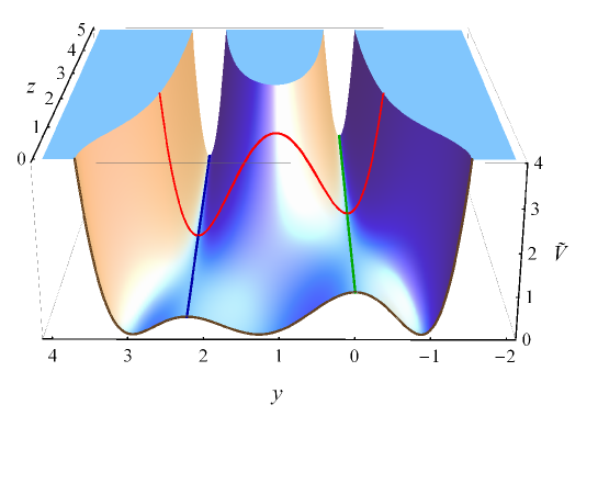
Figure 1: The dimensionless potential $\tilde{V}=V/\kappa^{2}M^{4}$ versus $y$ and $z$ for $\xi=0.3$. The red curve at $z=2$ clearly shows one maximum at $y\sim 1$ and two minima at $y_{1}=0$ (standard trajectory) and $y_{2}=2/3\xi=0.22$ (shifted trajectory). These minima become maxima near $z=0$ as are shown by the brown curve.

Along the shifted trajectory SUSY is broken due to the presence of a non-zero vacuum energy density $\kappa^{2}M^{4}(1-4/27\xi^{2})^{2}$. This in turn generates the radiative corrections which can lift the flatness of the $y_{2}$ trajectory while providing the necessary slope for driving inflation. In order to calculate the one-loop radiative correction at $y_{2}$ we need to compute the mass spectrum of the model along this path where both $SU(5)$ gauge symmetry and SUSY are broken.

During inflation, the field $\Phi$ acquires a vev in the $\phi_{24}$ direction which breaks the $SU(5)$ gauge symmetry down to SM gauge group $G_{SM}$. Perturbing around this vacuum $v_{2}=2My_{2}$ and replacing $\phi_{24}\rightarrow\left[v_{2}+Re(\phi_{24})+i\,Im(\phi_{24})\right]/\sqrt{2}$, the potential in Eq. (4) yields the following masses for real scalar fields, $Re(\phi_{24})$ and $Im(\phi_{24})$:

$$m^{2}_{24_{\pm}}=\pm\kappa^{2}M^{2}(\frac{4}{27\xi^{2}}-1)+\kappa^{2}|S|^{2}.$$ (13)

The superpotential in Eq. (3) generates a Weyl fermion with mass-squared:

$$m_{24}^{2}=\kappa^{2}|S|^{2}.$$ (14)

Similarly, we obtain the following masses for the real scalar fields $Re(\phi_{i})$ and $Im(\phi_{i})$ with $i=1,...,8,21,22,23$:

$$m^{2}_{i_{\pm}}=\pm 5\kappa^{2}M^{2}(\frac{4}{27\xi^{2}}-1)+25\kappa^{2}|S|^{2},$$ (15)

and from the following terms of the superpotential

$$\delta W=\kappa S\left(M^{2}-\frac{1}{2}\phi_{i}^{2}-\frac{3\beta}{4\kappa M_{*}}d_{i\,i\,24}\phi_{i}^{2}\phi_{24}\right),$$ (16)

the $11$ weyl fermions $\psi_{i}$, $i=1,...,8,21,22,23$, acquire a universal mass-squared:

$$m^{2}_{i}=25\kappa^{2}|S|^{2}.$$ (17)

It is worth noting that the SUSY breaking along the inflationary trajectory, which is due to the non zero vacuum energy $\kappa^{2}M^{4}(1-\frac{4}{27\xi^{2}})^{2}$, generates a mass splitting in $\phi_{24}$ supermultiplet and in $\phi_{i}$, $i=1,...,8,21,22,23$, supermultiplets. This is the only place where mass splitting between fermions and bosons appears.

The $D$-term contribution to the masses of scalar fields $\phi_{i}$, $i=9,...,20$, is obtained from the following term:

$$g^{2}\left(f^{ijk}\phi_{j}\phi^{{\dagger}}_{k}\right)\left(f^{ilm}\phi_{l}\phi^{{\dagger}}_{m}\right),$$ (18)

where $g$ is the $SU(5)$ gauge coupling. As an example, we obtain the mass of $\phi_{10}$ field as follows:

$$\frac{1}{2}\,g^{2}\left(f^{9\,24\,10}v_{2}\phi_{10}+f^{9\,10\,24}v_{2}\phi^{{\dagger}}_{10}\right)^{2},$$ (19)

which leads to mass-squared $\frac{25}{30}g^{2}v_{2}^{2}$ using $f^{9\,10\,24}=-f^{9\,24\,10}=\frac{1}{2}\sqrt{\frac{5}{3}}$ and $f^{i\,10\,24}=0$ for $i=10,...,20$. Thus, the D term contributes with a universal mass-squared $\frac{25}{30}g^{2}v_{2}^{2}$ for the above mentioned $12$ real scalar fields. The mixing between chiral fermions $\psi_{i}$, $i=9,....,20$, and the gauginos $\lambda_{i}$, $i=9,....,20$, gives rise to Dirac mass term:

$$i\sqrt{2}gf^{ijk}\left(\phi^{{\dagger}}_{k}\lambda_{i}\psi_{j}+\bar{\psi}_{k}\bar{\lambda}_{i}\phi_{j}\right).$$ (20)

This leads to $12$ Dirac fermions with mass-squared $\frac{25}{30}g^{2}v_{2}^{2}$. Finally, the gauge bosons $A_{\mu}^{i}$, $i=9,...,20$, acquire masses from the following term:

$$g^{2}f^{ijk}f^{ilm}A_{\mu}^{j}A^{l\mu}\phi^{{\dagger}}_{k}\phi_{m}.$$ (21)

This generates a universal mass-squared $\frac{25}{30}g^{2}v_{2}^{2}$ for all $12$ gauge bosons.

In Table 1, we summarize the results of the mass spectrum of the model along the shifted inflationary trajectory. As noted above, the mass splitting only occurs in $\phi_{24}$ and $\phi_{i}$, $i=1,...,8,21,22,23$, supermultiplets which contain 12 Majorana fermions with two degrees of freedom and 24 real scalars, whereas there is no mass splitting in $\phi_{i}$, $i=9,...,20$, supermultiplets which consist of 12 massive Dirac fermions with four degrees of freedom, 12 massive gauge bosons with 3 degrees of freedom, and 12 real scalars. It can be readily checked that all these supermultiplets satisfy the supertrace rule $StrM^{2}=0$.

Fields	Squared Masses
2 real scalars	$\kappa^{2}|S|^{2}\pm\kappa^{2}M^{2}(\frac{4}{27\xi^{2}}-1)$
1 Majorana fermion	$\kappa^{2}|S|^{2}$
22 real scalars	$25\kappa^{2}|S|^{2}\pm 5\kappa^{2}M^{2}(\frac{4}{27\xi^{2}}-1)$
11 Majorana fermions	$25\kappa^{2}|S|^{2}$
12 real scalars	$\frac{25}{30}g^{2}v_{2}^{2}$
12 Dirac fermions	$\frac{25}{30}g^{2}v_{2}^{2}$
12 gauge bosons	$\frac{25}{30}g^{2}v_{2}^{2}$

Table 1: The mass spectrum of the shifted hybrid $SU(5)$ model as the system moves along the inflationary trajectory $y_{2}$ ($v_{2}=2\,M\,y_{2}=\frac{4\,M}{3\,\xi}$).

The inflationary effective potential with 1-loop radiative correction is given by

$$V_{\rm 1loop}\!\! \!=\! \!\!\kappa^{2}M_{\xi}^{4}\left(1+\frac{\kappa^{2}}{16\pi^{2}}\left[F(M_{\xi}^{2},x^{2})+11\times 25\,F(5M_{\xi}^{2},5\,x^{2})\right]\right),$$ (22)

where

$$F(M_{\xi}^{2},x^{2})=\frac{1}{4}\left(\left(x^{4}+1\right)\ln\frac{\left(x^{4}-1\right)}{x^{4}}+2x^{2}\ln\frac{x^{2}+1}{x^{2}-1}+2\ln\frac{\kappa^{2}M_{\xi}^{2}x^{2}}{Q^{2}}-3\right),$$ (23)

$x=|S|/M_{\xi}$, $M_{\xi}^{2}=M^{2}(4/27\xi^{2}-1)$ and $Q$ is the renormalization scale. The spectrum of the model at the $SU(5)$ breaking SUSY minimum is given by the massless octet $\phi_{i}$, $i=1,..,8$, and triplet $\phi_{k}$, $k=21,22,23$ scalars/fermions, while the fields $\phi_{j}$, $j=9,...,20$, acquire mass-squared of order $g^{2}v_{2}^{2}$. Finally $\phi_{24}$ and $S$ fields acquire masses of order $\kappa M$. As will be shown later, these octets and triplets spoil the gauge coupling unification and we, therefore, need to add some vector-like matter to preserve unification. Before discussing unification we consider the contribution from sugra corrections.

2.1 Sugra corrections and non-minimal Kähler potential

We take the following general form of Kähler potential:

$$K = |S|^{2}+Tr|\Phi|^{2}+|H|^{2}+|\bar{H}|^{2}$$ (24)

$$+\kappa_{S\Phi}\frac{|S|^{2}\,Tr|\Phi|^{2}}{m_{P}^{2}}+\kappa_{SH}\frac{|S|^{2}|H|^{2}}{m_{P}^{2}}+\kappa_{S\bar{H}}\frac{|S|^{2}|\bar{H}|^{2}}{m_{P}^{2}}$$

$$+\kappa_{H\Phi}\frac{|H|^{2}\,Tr|\Phi|^{2}}{m_{P}^{2}}+\kappa_{\bar{H}\Phi}\frac{|\bar{H}|^{2}\,Tr|\Phi|^{2}}{m_{P}^{2}}+\kappa_{H\bar{H}}\frac{|H|^{2}|\bar{H}|^{2}}{m_{P}^{2}}$$

$$+\kappa_{S}\frac{|S|^{4}}{4m_{P}^{2}}+\kappa_{\Phi}\frac{(Tr|\Phi|^{2})^{2}}{4m_{P}^{2}}+\kappa_{H}\frac{|H|^{4}}{4m_{P}^{2}}+\kappa_{\bar{H}}\frac{|\bar{H}|^{4}}{4m_{P}^{2}}$$

$$+\kappa_{SS}\frac{|S|^{6}}{6m_{P}^{4}}+\kappa_{\Phi\Phi}\frac{(Tr|\Phi|^{2})^{3}}{6m_{P}^{4}}+\kappa_{HH}\frac{|H|^{6}}{6m_{P}^{4}}+\kappa_{\bar{H}\bar{H}}\frac{|\bar{H}|^{6}}{6m_{P}^{4}}+\cdots,$$

where $m_{P}\simeq 2.4\times 10^{18}$ GeV is the reduced Planck mass. Additionally, for the sake of simplicity, the contribution of many other terms e.g., of the form

$$c_{2}\,[Tr(\Phi^{2})+h.c.]+c_{3}\,[Tr(\Phi^{3})/m_{P}+h.c.]+\cdots$$ (25)

is assumed to be zero. Alternatively we can effectively absorb these extra contributions coming from the $\Phi$ superfield into various couplings of the above Kähler potential as only the $|S|$ field plays an active role during inflation. The sugra scalar potential is given by

$$V_{F}=e^{K/m_{P}^{2}}\left(K_{i\bar{j}}^{-1}D_{z_{i}}WD_{z^{*}_{j}}W^{*}-3m_{P}^{-2}\left|W\right|^{2}\right),$$ (26)

with $z_{i}$ being the bosonic components of the superfields $z_{i}\in\{S,\Phi,H,\bar{H},\cdots\}$ and where we have defined

$$D_{z_{i}}W\equiv\frac{\partial W}{\partial z_{i}}+m_{P}^{-2}\frac{\partial K}{\partial z_{i}}W,\,\,\,K_{i\bar{j}}\equiv\frac{\partial^{2}K}{\partial z_{i}\partial z_{j}^{*}},$$ (27)

and $D_{z_{i}^{*}}W^{*}=\left(D_{z_{i}}W\right)^{*}.$ Now in the inflationary trajectory with the D-flat direction ($\phi_{i}=\phi_{i}^{*}$, $|\bar{H}_{a}|=|H_{a}|$) and using Eqs. (3), (22), (24), and (26), we obtain the following form of the full potential:

$$V = \kappa^{2}M_{\xi}^{4}\left(1+\frac{\kappa^{2}}{16\pi^{2}}\left[F(M_{\xi}^{2},x^{2})+11\times 25\,F(5M_{\xi}^{2},5\,x^{2})\right]\right.$$ (28)

$$+\left(\frac{4(1-\kappa_{S\Phi})}{9\,(4/27-\xi^{2})}-\kappa_{S}\,x^{2}\right)\left(\frac{M_{\xi}}{m_{P}}\right)^{2}$$

$$\left.+\left(\frac{4((1-2\kappa_{S\Phi})^{2}+1+\kappa_{\Phi})}{81\,(4/27-\xi^{2})^{2}}\right.\right.$$

$$\left.\left.+\frac{4((1-\kappa_{S\Phi})^{2}-\kappa_{S}(1-2\kappa_{S\Phi}))x^{2}}{9\,(4/27-\xi^{2})}+\frac{\gamma_{S}\,x^{4}}{2}\right)\left(\frac{M_{\xi}}{m_{P}}\right)^{4}+\cdots\right)+\cdots\,,$$

where $x=|S|/M_{\xi}$, $M_{\xi}^{2}=M^{2}(4/27\xi^{2}-1)$ and $\gamma_{S}=1-\frac{7\kappa_{S}}{2}+2\kappa_{S}^{2}-3\kappa_{SS}$. We restrict ourselves to $\kappa\gtrsim 10^{-3}$ and neglect contribution of soft SUSY breaking terms assuming soft masses of order 1 TeV [6, 21, 22].

Before proceeding further, let us consider the possible mass contribution from the non-minimal terms of the Kähler potential. In particular, as we will see, the $SU(2)$ triplet and $SU(3)$ octet multiplets remain massless as a consequence of both $R$ and $SU(5)$ gauge symmetries. To see this explicitly, consider the following general form of the fermionic mass matrix:

$$({\cal M}_{F})_{ij}=e^{K/2}\left(W_{ij}+K_{ij}W+K_{i}W_{j}+K_{j}W_{i}+K_{i}K_{j}W-K^{k\overline{l}}K_{ij\overline{l}}D_{k}W\right).$$ (29)

Since, in the SUSY minimum $W$ and $W_{i}$ essentially vanish due to R-symmetry, the triplet and octet multiplets therefore do not acquire masses from the above contribution. The other possible contribution to fermionic masses come through the mixing of chiral fermions and gauginos,

$$i\,g\,\sqrt{2}\,f^{i\,j\,k}\,\left(\phi_{k}\,\psi_{\bar{l}}\,K_{{\bar{l}}j}\lambda_{i}+\bar{\psi}_{\bar{l}}\,K_{{\bar{l}}k}\,\bar{\lambda}_{i}\,\phi_{j}\right).$$ (30)

Due to $SU(5)$ gauge symmetry, these terms also vanish for the triplet and octet multiplets. (Note that $f^{i\,j\,24}=0$ for the triplet and octet states). Therefore, both the fermionic and bosonic masses of these multiplets vanish as a consequence of $R$-symmetry and SUSY $SU(5)$. However, these multiplets can acquire TeV scale masses as is discussed in more detail in the third section.

On the other hand, in the shifted trajectory case a non-zero mass contribution is expected from the nonminimal terms of the Kähler potential. But these contributions are expected to have a negligible effect on the inflationary predictions as they appear inside the logarithmic functions of radiative corrections. Therefore, in numerical calculations we can safely ignore these contributions.

Before starting our discussion of this model it is useful to recall here the basic results of the slow roll assumption. The inflationary slow-roll parameters are given by

$$\epsilon=\frac{m_{P}^{2}}{4\,M_{\xi}^{2}}\left(\frac{\partial_{x}V}{V}\right)^{2},\,\,\,\eta=\frac{m_{P}^{2}}{2\,M_{\xi}^{2}}\left(\frac{\partial_{x}^{2}V}{V}\right).$$ (31)

In the slow-roll approximation (i.e. $\epsilon$, $|\eta|\ll 1$), the scalar spectral index $n_{s}$ and the tensor to scalar ratio $r$ are given (to leading order) by

$$n_{s}\simeq 1+2\,\eta-6\,\epsilon,\,\,\,r\simeq 16\,\epsilon.$$ (32)

The number of e-folds during inflation $l_{0}=2\,\pi/k_{0}$ has crossed the horizon is given by

$$N_{0}=2\left(\frac{M_{\xi}}{m_{P}}\right)^{2}\int_{x_{e}}^{x_{0}}\left(\frac{V}{\partial_{x}V}\right)dx,$$ (33)

where $|S_{0}|=x_{0}\,M_{\xi}$ is the field value at the comoving scale $l_{0}$, and $x_{e}$ denotes the value of field at the end of inflation, defined by $|\eta(x_{e})|=1$ (or $x_{e}=1$). During inflation, this scale exits the horizon at approximately

$$N_{0}=53+\frac{1}{3}\ln\left(\frac{T_{r}}{10^{9}~{}{\rm GeV}}\right)+\frac{2}{3}\ln\left(\frac{V^{1/4}(x_{0})}{10^{15}~{}{\rm GeV}}\right),$$ (34)

where $T_{r}$ is the reheat temperature and for a numerical work we will set $T_{r}=10^{9}$ GeV. This could easily be reduced to lower values if the gravitino problem is regarded to be an issue. The subscript ‘0’ denotes the comoving scale corresponding to $k_{0}=0.002$ Mpc^-1. The amplitude of the curvature perturbation is given by

$$\Delta_{\mathcal{R}}^{2}=\frac{1}{24\,\pi^{2}}\left.\left(\frac{V/m_{P}^{4}}{\epsilon}\right)\right|_{k=k_{0}},$$ (35)

where $\Delta_{\mathcal{R}}^{2}=(2.43\pm 0.11)\times 10^{-9}$ is the WMAP7 normalization at $k_{0}=0.002\,\rm{Mpc}^{-1}$ [13]. Note that, for added precision, we include in our calculations the first order corrections [24] in the slow-roll expansion for the quantities $n_{s}$, $r$, and $\Delta_{\mathcal{R}}$.

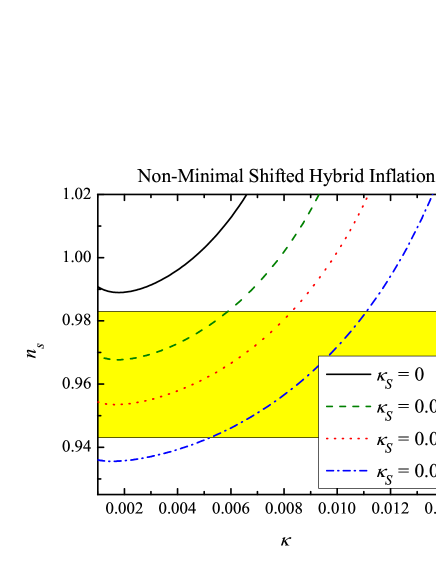
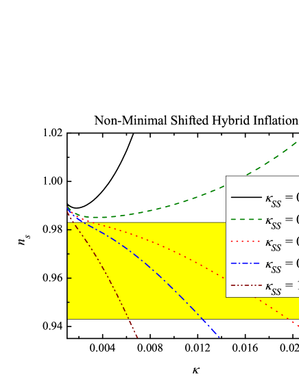
Figure 2: $n_{s}$ vs $\kappa$ for shifted hybrid inflation with $\xi=0.3$ and $T_{r}=10^{9}$ GeV. The WMAP7 1-$\sigma$ (68% confidence level) bounds are shown in yellow.

Including sugra correction, in general, introduces a mass squared term of order $H^{2}$, where $H\simeq\sqrt{V/3\,m_{P}^{2}}$ is the Hubble parameter. This in turn makes the slow parameter $\eta\sim 1$ and spoils inflation. This is the well known $\eta$ problem. However, in the case of supersymmetric shifted hybrid inflation with minimal Kähler potential this problem is naturally resolved due to a cancellation between the mass squared terms of the exponential factor and the other part of the potential in Eq. (26). The linear dependence of $W$ in $S$ due to $R$-symmetry guarantees this cancellation to all orders [3, 25]. With non-minimal Kähler potential the mass squared term can be approximated as

$$\sim\left(\kappa_{S}+\frac{4((1-\kappa_{S\Phi})^{2}-\kappa_{S}(1-2\kappa_{S\Phi}))}{9\,(4/27-\xi^{2})}\left(\frac{M_{\xi}}{m_{P}}\right)^{2}+\cdots\right)H^{2},$$ (36)

which can spoil inflation for $\kappa_{S}\sim 1$, but for reasonably natural values of parameters $\kappa_{S}\lesssim 0.01$ and $|\kappa_{S\Phi}|\lesssim 1$ we can obtain successful inflation consistent with WMAP7 data.

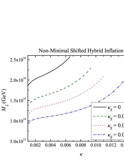
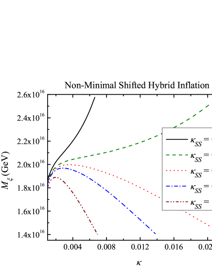
Figure 3: $M_{\xi}$ vs $\kappa$ for shifted hybrid inflation with $\xi=0.3$ and $T_{r}=10^{9}$ GeV.

The predicted values of various parameters for shifted hybrid inflation are displayed in Figs. 2, 3 and 4. For minimal Kähler potential the scalar spectral index $n_{s}\gtrsim 0.99$ lies outside the 1-$\sigma$ bounds of WMAP7 data. With non-minimal Kähler potential only $\kappa_{S}$ and $\kappa_{SS}$ play the important role of reducing the scalar spectral index to the central value of WMAP7 data, i.e. $n_{s}\simeq 0.96$. As can be seen in Fig. 2 we can obtain $n_{s}$ within the 1-$\sigma$ bounds of WMAP7 data for $\kappa_{S}\gtrsim 0.005$ or $0.33\lesssim\kappa_{SS}\lesssim 1$ with all other non-minimal parameters equal to zero.

The $\kappa_{S}\neq 0$ case has been considered previously in Ref. [18] for standard and smooth hybrid inflation. The results we obtain here are quite similar to the one obtained in Ref. [18]. In particular, the scalar spectral index is given by

$$n_{s}\simeq 1-2\,\kappa_{S}+\left(\frac{8(1-\kappa_{S})}{9\,(4/27-\xi^{2})}+6\gamma_{S}x_{0}^{2}\right)\left(\frac{M_{\xi}}{m_{P}}\right)^{2}-\frac{275\kappa^{2}}{16\,\pi^{2}}\left|\partial^{2}_{x_{0}}F(5\,x_{0}^{2})\right|\left(\frac{m_{P}}{M_{\xi}}\right)^{2}.$$ (37)

From Fig. 3 and Fig. 4 it is clear that the value of parameters $|S_{0}|/m_{P}$, $M_{\xi}/m_{P}$ and $x_{0}\left(=|S_{0}|/M_{\xi}\right)$ increases with $\kappa$. Therefore, the sugra contribution in the above expression raises the value of the scalar spectral index $n_{s}$ with $\kappa$. The radiative correction, on the other hand, does not vary much with $\kappa$ since both $|F^{\prime\prime}|$ ($\simeq\frac{1}{x_{0}^{2}}$ for large $x_{0}$) and $\left(\frac{m_{P}}{M_{\xi}}\right)^{2}$ tries to compensate the increase in $\kappa^{2}$ term, in above expression. For small values of $\kappa$ sugra correction is suppressed as compared to radiative correction and $-2\,\kappa_{S}$ factor, which reduces the scalar spectral index within the 1-$\sigma$ bounds of WMAP7 data.

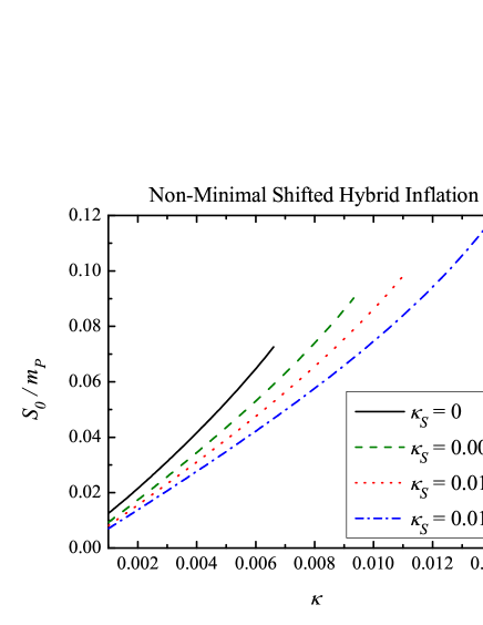
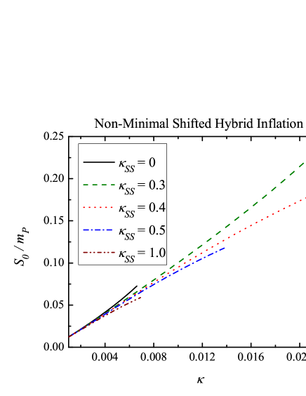
Figure 4: $S_{0}/m_{P}$ vs $\kappa$ for shifted hybrid inflation with $\xi=0.3$ and $T_{r}=10^{9}$ GeV.

For $\kappa_{SS}\neq 0$ case we obtain following result for the scalar spectral index:

$$n_{s}\simeq 1+\left(\frac{8}{9\,(4/27-\xi^{2})}+6\,(1-3\,\kappa_{SS})\,x_{0}^{2}\right)\left(\frac{M_{\xi}}{m_{P}}\right)^{2}-\frac{275\kappa^{2}}{16\,\pi^{2}}\left|\partial^{2}_{x_{0}}F(5\,x_{0}^{2})\right|\left(\frac{m_{P}}{M_{\xi}}\right)^{2}.$$ (38)

In this case with $\kappa_{SS}\lesssim 1/3\simeq 0.33$ sugra term is positive and raises the value of $n_{s}$ with $\kappa$. For small values of $\kappa$ (or $x_{0}$) radiative correction becomes important and a small reduction in $n_{s}$ is observed as shown in Fig. 2. On the other hand, for $\kappa_{SS}\gtrsim 0.33$, $\gamma_{S}$ becomes negative and we obtain a reduction in $n_{s}$ with $\kappa$ which is consistent with the WMAP7 data (see Fig. 3). With $\kappa_{SS}\gtrsim 0.33$ quadratic and quartic terms of the potential in Eq. (28) are positive and negative respectively. This provides a nice example of hilltop inflation [26] and a similar kind of potential has been analyzed in Refs. [27, 28, 29, 30]. The value of the tensor to scalar ratio $r\lesssim 10^{-5}$ remains small in the above model of shifted hybrid inflation. For realizing observable $r$ values in supersymmetric hybrid inflationary models see Ref. [19].

3 Gauge coupling unification and TeV scale vector-like matter

In this section we discuss the impact of the massless $SU(3)$ octet and $SU(2)$ triplet multiplets on the gauge coupling unification. After $SU(5)$ breaking, these multiplets remain massless in the limit of exact supersymmtery and may spoil gauge coupling unification. After inclusion of soft SUSY breaking mass terms taking account of $\langle S\rangle\sim$ TeV, these particles acquire masses of order TeV.

In order to achieve gauge coupling unification we can add suitable vectorlike particles with TeV scale masses. These vectorlike particles have recently been studied to solve the little hierarchy problem in the MSSM [31, 32, 33]. The requirement that the three gauge couplings should remain perturbative at least up to the unification scale and the value of strong coupling should lie within the experimental uncertainties [34], greatly reduces the choices of vectorlike combinations. Furthermore, in order to avoid fast proton decay we do not consider the triplet scalar Higgs vectorlike combination $D(3,1,-1/3)+D(\overline{3},1,1/3)$. Taking into account these considerations we choose the following combination of extra vectorlike particles:

$$L(1,2,1/2)+\overline{L}(1,2,-1/2)+2(E(1,1,1)+\overline{E}(1,1,-1)).$$ (39)

The sum of 1-loop beta function of octet $G(8,1,0)$, triplet $W(1,3,0)$ and the above vectorlike combination is $\Delta b=(0,0,3)+(0,2,0)+(3,1,0)=(3,3,3)$. The 2-loop beta functions and RGEs for SM, MSSM and these extra vectorlike particles can be found in Refs. [35, 36, 37, 38, 39].

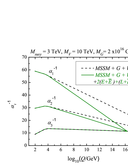
Figure 5: Gauge coupling evolution with the effective SUSY breaking scale $M_{susy}=200$ GeV (left panels), $M_{susy}=3$ TeV (right panels) and $\tan\beta=10$. Dotted (solid) lines correspond to $MSSM+G+W$ ($MSSM+G+W+(L+\overline{L})+2(E+\overline{E})$). The masses of $G$, $W$ and extra vectorlike particles are set equal to $M_{V}=1$ TeV (left panels) and $M_{V}=10$ TeV (right panels).

The evolution of three gauge couplings with and without the extra vectorlike particle combination (Eq. (39)) is shown in Fig. 5. Here we have used 2-loop RGEs with the SUSY breaking scale $M_{susy}=200$ GeV and $M_{susy}=3$ TeV and the masses of vectorlike particles $M_{V}=1$ TeV and $M_{V}=10$ TeV. The value of the strong gauge coupling is fixed by the gauge unification condition and is required to lie within the experimental uncertainties [34]. The GUT scale is found to lie in the range $M_{G}\sim(2-7)\times 10^{16}$ GeV for $M_{susy}\sim(0.2-3)$ TeV and $M_{V}\sim(1-10)$ TeV. These extra particles may be detected at the LHC provided their masses are less than or of order a TeV [40]. As an example, the gluon-gluon fusion channel can lead to $SU(3)$ octet pair production at the LHC:

$A^{\mu}_{i}\,A^{\mu}_{i}\,\longrightarrow\,\phi_{i}\,\phi_{i}\,\longrightarrow\,q\,\bar{q}\,\,\,(e^{+}\,e^{-}),$

where $i=1,...,8$. This coupling can be generated from the kinetic energy term of $\Phi$.

4 Summary

To summarize, we have analyzed the adjoint field hybrid inflationary model in supersymmetric $SU(5)$. Since the minimal SUSY $SU(5)$ hybrid inflation suffers from the monopole problem we have discussed $SU(5)$ shifted hybrid inflation. In this model the $SU(5)$ gauge symmetry is broken during inflation and monopoles are inflated away before inflation ends. In minimal shifted hybrid inflation the spectral index $n_{s}\gtrsim 0.99$ lies outside the WMAP7 1-$\sigma$ bounds with $\kappa\gtrsim 10^{-3}$ and TeV scale soft SUSY breaking masses. However, with a nonminimal Kähler potential the WMAP7 1-$\sigma$ region nicely compatible with shifted hybrid inflation. A tiny value of $r\lesssim 10^{-5}$ is obtained in this model. Furthermore, as a consequence of $R$-symmetry, the $SU(2)$ octet and $SU(3)$ triplet supermultiplets lie in the TeV range. In order to preserve gauge coupling unification we include additional TeV scale vectorlike particles which may be observed at the LHC.

References

- [1] A. D. Linde, Phys. Rev. D 49, 748 (1994) [arXiv:astro-ph/9307002].
- [2] G. R. Dvali, Q. Shafi and R. K. Schaefer, Phys. Rev. Lett. 73, 1886 (1994) [arXiv:hep-ph/9406319].
- [3] E. J. Copeland, A. R. Liddle, D. H. Lyth, E. D. Stewart and D. Wands, Phys. Rev. D 49, 6410 (1994) [arXiv:astro-ph/9401011].
- [4] V. N. Senoguz and Q. Shafi, Phys. Lett. B 567, 79 (2003) [arXiv:hep-ph/0305089].
- [5] V. N. Senoguz and Q. Shafi, Phys. Lett. B 596, 8 (2004) [arXiv:hep-ph/0403294].
- [6] V. N. Senoguz and Q. Shafi, Phys. Rev. D 71, 043514 (2005) [arXiv:hep-ph/0412102].
- [7] R. Jeannerot and M. Postma, JHEP 0505, 071 (2005) [arXiv:hep-ph/0503146].
- [8] C. Pallis, arXiv:0710.3074 [hep-ph].
- [9] S. Antusch, K. Dutta and P. M. Kostka, Phys. Lett. B 677, 221 (2009) [arXiv:0902.2934 [hep-ph]].
- [10] S. Antusch, M. Bastero-Gil, J. P. Baumann, K. Dutta, S. F. King and P. M. Kostka, JHEP 1008, 100 (2010) [arXiv:1003.3233 [hep-ph]].
- [11] D. H. Lyth and A. Riotto, Phys. Rept. 314, 1 (1999) [arXiv:hep-ph/9807278]; G. Lazarides, Lect. Notes Phys. 592, 351 (2002) [arXiv:hep-ph/0111328]; A. Mazumdar and J. Rocher, arXiv:1001.0993 [hep-ph], for a recent review.
- [12] R. Jeannerot, S. Khalil, G. Lazarides and Q. Shafi, JHEP 0010, 012 (2000) [arXiv:hep-ph/0002151].
- [13] E. Komatsu et al. [WMAP Collaboration], Astrophys. J. Suppl. 192, 18 (2011) [arXiv:1001.4538 [astro-ph.CO]].
- [14] C. Panagiotakopoulos, Phys. Rev. D 55, R7335 (1997) [arXiv:hep-ph/9702433]; W. Buchmuller, L. Covi and D. Delepine, Phys. Lett. B 491, 183 (2000) [arXiv:hep-ph/0006168].
- [15] A. D. Linde and A. Riotto, Phys. Rev. D 56, R1841 (1997) [arXiv:hep-ph/9703209].
- [16] M. Kawasaki, M. Yamaguchi and J. Yokoyama, Phys. Rev. D 68, 023508 (2003) [arXiv:hep-ph/0304161].
- [17] M. Bastero-Gil, S. F. King and Q. Shafi, Phys. Lett. B 651, 345 (2007) [arXiv:hep-ph/0604198].
- [18] M. ur Rehman, V. N. Senoguz and Q. Shafi, Phys. Rev. D 75, 043522 (2007) [arXiv:hep-ph/0612023].
- [19] Q. Shafi and J. R. Wickman, Phys. Lett. B 696, 438 (2011) [arXiv:1009.5340 [hep-ph]]; M. U. Rehman, Q. Shafi and J. R. Wickman, arXiv:1012.0309 [astro-ph.CO].
- [20] L. Covi, G. Mangano, A. Masiero and G. Miele, Phys. Lett. B 424, 253 (1998) [arXiv:hep-ph/9707405].
- [21] M. U. Rehman, Q. Shafi and J. R. Wickman, Phys. Lett. B 683, 191 (2010) [arXiv:0908.3896 [hep-ph]].
- [22] M. U. Rehman, Q. Shafi and J. R. Wickman, Phys. Lett. B 688, 75 (2010) [arXiv:0912.4737 [hep-ph]].
- [23] K. Nakayama, F. Takahashi and T. T. Yanagida, JCAP 1012, 010 (2010) [arXiv:1007.5152 [hep-ph]].
- [24] V. N. Senoguz and Q. Shafi, Phys. Lett. B 668, 6 (2008) [arXiv:0806.2798 [hep-ph]].
- [25] E. D. Stewart, Phys. Rev. D 51, 6847 (1995) [arXiv:hep-ph/9405389].
- [26] L. Boubekeur and D. H. Lyth, JCAP 0507, 010 (2005) [arXiv:hep-ph/0502047].
- [27] K. Kohri, C. M. Lin and D. H. Lyth, JCAP 0712, 004 (2007) [arXiv:0707.3826 [hep-ph]].
- [28] C. M. Lin and K. Cheung, Phys. Rev. D 79, 083509 (2009) [arXiv:0901.3280 [hep-ph]].
- [29] C. Pallis, JCAP 0904, 024 (2009) [arXiv:0902.0334 [hep-ph]].
- [30] M. U. Rehman, Q. Shafi and J. R. Wickman, Phys. Rev. D 79, 103503 (2009) [arXiv:0901.4345 [hep-ph]].
- [31] K. S. Babu, I. Gogoladze, M. U. Rehman and Q. Shafi, Phys. Rev. D 78, 055017 (2008) [arXiv:0807.3055 [hep-ph]].
- [32] S. P. Martin, Phys. Rev. D 81, 035004 (2010) [arXiv:0910.2732 [hep-ph]].
- [33] P. W. Graham, A. Ismail, S. Rajendran and P. Saraswat, Phys. Rev. D 81, 055016 (2010) [arXiv:0910.3020 [hep-ph]].
- [34] C. Amsler et al. (Particle Data Group), Physics Letters B667, 1 (2008).
- [35] M. E. Machacek and M. T. Vaughn, Nucl. Phys. B 222, 83 (1983); Nucl. Phys. B 236, 221 (1984); Nucl. Phys. B 249, 70 (1985).
- [36] G. Cvetic, C. S. Kim and S. S. Hwang, Phys. Rev. D 58, 116003 (1998).
- [37] V. D. Barger, M. S. Berger and P. Ohmann, Phys. Rev. D 47, 1093 (1993); Phys. Rev. D 49, 4908 (1994).
- [38] S. P. Martin and M. T. Vaughn, Phys. Rev. D 50, 2282 (1994).
- [39] V. Barger, N. G. Deshpande, J. Jiang, P. Langacker and T. Li, Nucl. Phys. B 793, 307 (2008) [arXiv:hep-ph/0701136].
- [40] T. Han, I. Lewis and Z. Liu, JHEP 1012, 085 (2010) [arXiv:1010.4309 [hep-ph]], and references therein.