Interference detection in gaussian noise

Abstract

Interference detection in gaussian noise is proposed. It can be applied for easy detection and editing of interference lines in radio spectral line observations. One need not know the position of occurence or keep track of interference in the band. Results obtained on real data have been displayed.

1 Introduction

Radio Frequency Interference(RFI) is a common problem during radio spectral line observations. This RFI can be edited manually by inspecting the individual power spectra. RFI lines can appear at various positions in the spectrum depending upon the nature of the interference or the instrument settings. Here a few methods of detection have been proposed which apply to the power spectrum(i,e after the fourier transform of the recorded data) so that the RFI can be detected and edited using an algorithm. Using such an RFI detection algorithm one can analyse huge amounts of data with minimum time and effort. The method has been described as it applies to radio spectral line observations using dual Dicke switching[1].

2 The Radio spectral line observation

In a typical radio spectral line observation one first decides upon the frequency at which the line will be observed. The bandwidth required to detect the line or lines and the period for which the observation will be made. This period decides the signal to noise ratio in the final spectrum. The line is assumed to be observed with the procedure of dual Dicke switching. In this observation procedure the band is split into two equal parts. The spectral line is made to appear in these two parts alternately by appropriately tuning the telescope. This is usually done by selecting two fixed local oscillator(LO) frequencies LO1 and LO2 over a period of time so that the gain characteristics of the instrument do not change significantly. Hence the observation consists of two types of spectra one with the spectral line appearing in the right part & the other with the spectral line in the left part. The first is called the $T_{on}$ spectrum & the other will be called the $T_{off}$ spectrum respectively. Typical power spectra appear as shown in the fig-1.

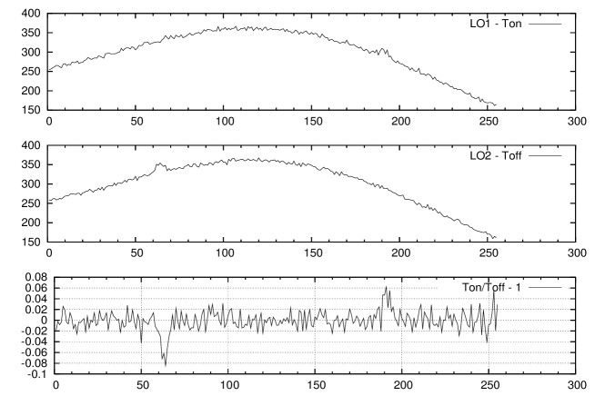
Figure 1: Typical simulated power spectra with dual Dicke switching at tuning frequencies LO1 and LO2, and their combination $T_{on}/T_{off}-1$. Abscissa is the channel number and the ordinate is arbitrary power. The spectral lines near channels 50(for Ton) and 200(for Toff) have been highly exagerated for the sake of clarity.

To detect the astronomical spectral line one is to first get rid of the background power(the band profile, refer fig-1, which is essentially the background radio power multiplied by the gain of the instrument) and normalize for the gain across the band. This can be acheived by simply doing a substraction of $T_{off}$ from $T_{on}$, since both have the same band profile. It is assumed that the bandshape of the instrument does not change appreciably for the two settings of the LO. The gain can be normalised by dividing the $T_{on}$-$T_{off}$ by $T_{off}$, the noisy features of $T_{off}$ in the denominator are not going to affect the ratio seriously since the derivative of $1/x$ goes as $1/x^{2}$(here $x$ is $T_{off}$). The main portion of the band where the lines are expected to appear has relatively higher magnitudes than the noise features. This can be seen in fig-1. The resulting output can be written as,

$$PS=\frac{T_{on}-T_{off}}{T_{off}}$$ (1)

PS consists of two lines(bottom panel in fig-1), one from $T_{on}$ and the other from $T_{off}$. The spectral line from $T_{off}$ will be inverted since $-ve$ of $T_{off}$ was added to $T_{on}$. PS is assumed to be gaussian noise(or approximately gaussian) with an inherent baseline. Noise characteristics of real data have been displayed in fig-10. Since there is no difference between addition or substraction of gaussian noise due to its symmetry, both lead to gaussian noise again. After this PS is folded and averaged appropriately so that the inverted line overlaps with the one in the other part. Ofcourse a negative of the inverted part will be added. This completes the simple data processing. Many such spectra collected over time can be added to improve the signal to noise ratio which eventually results in spectral line detection. It is the property of gaussian noise that the rms(root mean square) of the averaged spectrum reduces by a factor of $1/\sqrt{n}$ when n spectra are averaged[1].

2.1 Interference

RFI is a common enemy of spectral line observation. It can be produced in a variety of ways, by electrical sparking, computers, electronic gadgets etc. The magnitude of interference can be both small as well as large. It is easy to detect the large interference while the small interference is the one which is to be tackled. A typical interference infected spectrum is as shown in the fig-2(some times it is low enough that it is distinguishable only in the ratio $(T_{on}-T_{off})/T_{off}$).

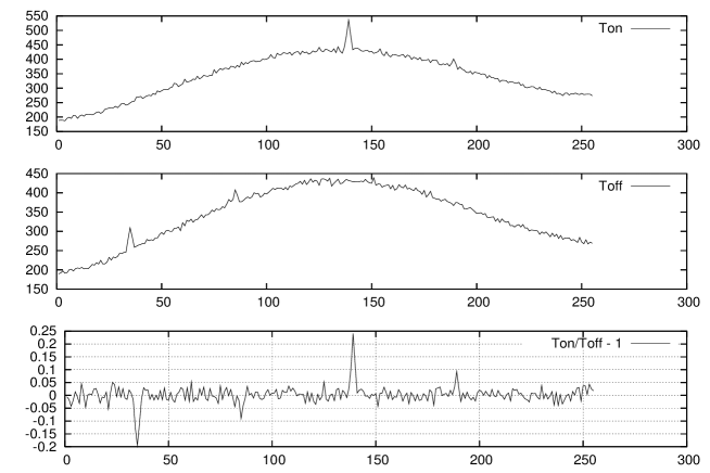
Figure 2: Typical power spectra with a couple of interference lines appearing in Ton at $\sim$140 and $\sim$180. Here the amplitude has been chosen to be small, in reality it can be both much higher or smaller.

Different sources produce different types of RFI. For example the RFI generated by electrical sparking will produce a series of lines. In such cases the standard deviation of the data itself may increase drastically. Using this information such data can be discarded. While some other electronic equipment may produce a single or multiple number of lines at some fixed position or positions in the band. In such cases one has to devise RFI excision techniques.

3 RFI Detection

The RFI lines appearing in the power spectrum can be recognized manually by carefully inspecting it. This would be laborious and time consuming. With the methods described here interference can be detected within the analysis program to auto recognize them. By an appropriate algorithm one can also have them edited(this is left to the user). This reduces manual labor as well as results in speedy data anaysis. In the methods proposed here the following assumptions have been made,

1. The RFI can be observed in a short integration time where as the detection of the astronomical signal would require a much longer integration time. In other words the spectrum subjected to interference detection satisfies the criteria that the astronomical line is smaller than or comparable to the standard deviation of the spectra.

2. The RFI is narrow band, i.e only a small portion or portions of the band are infected with it. It is necessary to use a portion of the band to find the standard deviation of the spectrum. This parameter is necessary in the detection of interference. The standard deviation is an important quantity relevant to noise.

3. It is also not necessary that the RFI be time variable. If the spectrum has interference as per the technique used here the associated channels will be flagged or else they will pass unflagged.

The technique to detect RFI depends on the properties of gaussian noise. When pure gaussian noise across N channels is considered there exists an expected maximum value that can occur across the channels. Similarly there exists for N channels a maximum for the difference between two adjacent channels. Lastly another quantity of interest is the added difference which is the sum of consecutive differences of similar sign( i.e the adjacent differences could be either -ve or +ve ). Suppose these difference signs go like + - + - + + - , then the fifth and sixth differences will be added to form one quantity. These quantities can be calculated theoretically and used to inspect the gaussian noise. Typical interference being sharp and narrow would produce, large channel values or differences between adjacent channel values that deviate considerably from the expected values. On such an occurence the corresponding channel or channels can be flagged for interference. The first quantity, expected maximum can be of use when the spectrum has reasonably zero mean all across the spectrum, in other words it has zero baseline, so is of less importance. The other two quantities are free from this defect as they are differences between adjacent channels which more or less have the same DC value. The methods using these three quantities have been named as direct,difference and added difference methods. The added difference traps those interference lines that escape the difference method due to their being slightly broad. Plots of these quantities signifying there use to detect interference have been given in the following sections.

3.1 Direct Method

This is the simplest of all the methods. In this method the spectrum of $N_{data}$ channels is divided into $n_{blk}$ number of blocks. Each block has now

$$N_{blk}=\frac{N_{data}}{n_{blk}}$$ (2)

number of data points. The block with the minimum standard deviation will be considered to be the representative of good data, meaning to say free of any interference. This is consistent in the sense that in the regions without any signal one has only noise, any interference introduced into this data will increase the standard deviation through increase in the mean value. The minimum standard deviation block will be used as a reference to calculate the required parameters to detect interference as well as to edit and repair it(one can replace the edited portion appropriately with noise of same standard deviation as that in the reference block). The absolute maximum value in this block can be used to generate a limit on the maximum absolute value that could be encountered in the other blocks by choosing a suitable multiplicative factor. This can also be done as the expected maximum is directly proportional to the standard deviation. Or else use the formula given below for $X_{mx}$ along with the standard deviation in the reference block and the total number of channels($N_{data}$). It should be noted that a constant muliplicative factor($>1$, say 1.1 - 1.3) has to be used with the expected maximum value to allow for the realistic departures from the expected value. If any block has any channel or channels with absolute value greater than this, then those channels in that block can be flagged for interference. The expected maximum absolute value for a N channel gaussian noise with zero mean is given by

$$\left<X_{mx}\right>=\sigma\sqrt{2}\ \int_{0}^{1}erf^{-1}(s^{\frac{1}{N}})\ ds$$ (3)

which has a convenient approximation as,

$$\left<X_{mx}\right>\approx\sigma\sqrt{2}\ erf^{-1}(1-\frac{0.5833}{N})$$ (4)

Derivation of this has been discussed in the appendix. This method requires that the spectrum under investigation be symmetrically distributed about the zero line. This can be brought about by calculating the mean of all the channels of the data and substracting it from each channel value of the spectrum. Also in some cases a baseline should be removed from the spectrum before subjecting to RFI detection. In the case where the interference is present this is difficult since the fitted curve will be baised by the interference line. If one is sure that the spectrum has no baseline then one can use this method or else omit it. However the following methods are more tolerant towards this.

3.2 Difference Method

The difference method is a simple method of interference detection. In this method adjacent channel differences all across a single spectrum will be found. For a N channel gaussian noise there exists an upper limit on the maximum expected difference. Which will be used as a reference to limit the maximum value that could be encountered across the N channels. Further the spectrum is divided into $n_{blk}$ blocks. Again the reference block will be the minimum standard deviation block. In each block the adjacent differences are found. A typical plot of differences of an interference infected $T_{on}/T_{off}-1$ spectrum is shown in the fig-3 which relates to the spectrum in fig-2.

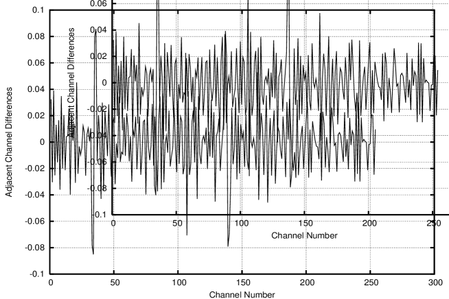
Figure 3: A plot of differences across the spectrum for a typical interference infected $(T_{on}-T_{off})/T_{off}$. The large differences in the interference infected region can be noticed.

Obviously the differences in the interference infected channels are much higher than the differences in the other channels. The expected value of the maximum difference($<D_{mx}>$) for gaussian noise with N data points is given by the relation,

$$\left<D_{mx}\right>\approx 2\sigma\!\!\int_{0}^{1}\!\!erf^{-1}(s^{\frac{1}{N}})\>{{d}}s=\sqrt{2}\left<X_{mx}\right>$$ (5)

where $\sigma$ can be taken from reference block. The derivation of this has been discussed in the appendix.

3.3 Added Difference Method

The added difference method is similar to the difference method except now the consecutive differences with same sign will be added to form a new array of quantities. Suppose the difference signs go like + - + - + + - , then the fifth and sixth differences will be added to form one quantity. The plot of such an array for a typical interference infected spectrum is shown in the fig-4 relating to fig-2. The improvement of interference detection criteria is clearly visible in this plot. Added difference method traps those interference lines which escape the difference method due to their being slightly broad. For this method the constraining limit($<Q_{mx}>$) can be obtained by finding the maximum added difference in the reference block and use a suitable multiple($>1$) of this or else use the empirical formula below,

$$<Q_{mx}>=2\ \sigma\ erf^{-1}\left(1-\frac{0.5833}{2N}\right).$$ (6)

Figure 4: A plot of added-differences array for the previous interference infected $(T_{on}-T_{off})/T_{off}$ spectrum. The improvement in the detection criteria compared to the differences in fig-3 is clearly apparent.

Appendix A Derivation of the expected maximum value for the gaussian distribution

Figure 5: Calculating the maximum expected value in N channel gaussian noise.

Considering N channels which produce gaussian noise(fig-5) of the same standard deviation $\sigma$. The probability that an absolute maximum value of c is produced in these channels is

$$p(c)=\frac{2^{N}Ne^{-\frac{c^{2}}{{2\sigma^{2}}}}}{{\left(\sigma\sqrt{2\pi}\right)}^{N}}\!\!\int_{0}^{c}e^{-\frac{{x_{2}}^{2}}{{2\sigma^{2}}}}{{d}}x_{2}\!\!\int_{0}^{c}e^{-\frac{{x_{3}}^{2}}{{2\sigma^{2}}}}{{d}}x_{3}\dots{{d}}x_{N}$$ (7)

which is nothing but the integral over all the possibilities over the remaining N-1 channels keeping one of the channels fixed at c. The factor $2^{N}$ is due to the fact that both +ve & -ve values are possible in each channel. The remaining N-1 channels are allowed to take all the values between -c and +c. N in the numerator appears as there are N-ways to fix a channel value to c. Each of the above integrals evaluates to $\sigma\sqrt{\pi/2}erf(c/{\sigma\sqrt{2}})$ resulting in,

$$p(c)=\frac{2Ne^{-\frac{c^{2}}{{2\sigma^{2}}}}}{\sigma\sqrt{2\pi}}{\left[erf{\left(\frac{c}{\sigma\sqrt{2}}\right)}\right]}^{N-1}$$ (8)

Now the maximum expected value can be written as,

$$\left<X_{mx}\right>=\!\!\int_{0}^{\infty}c\ p(c){{d}}c$$ (9)

$$\left<X_{mx}\right>=\frac{2N}{\sigma\sqrt{2\pi}}\!\!\int_{0}^{\infty}c\ e^{-\frac{c^{2}}{2\sigma^{2}}}{\left[erf{\left(\frac{c}{\sigma\sqrt{2}}\right)}\right]}^{N-1}{{d}}c$$ (10)

which can also be written using the derivative of $S=\left[erf\left(\frac{c}{\sigma\sqrt{2}}\right)\right]^{N}$ and expressing c in terms of S as

$$\left<X_{mx}\right>=\sigma\sqrt{2}\!\!\int_{0}^{1}erf^{-1}\left(S^{\frac{1}{N}}\right){{d}}S$$ (11)

which has an approximation

$$\left<X_{mx}\right>\approx\sigma\sqrt{2}\ erf^{-1}\left(1-\frac{0.5833}{N}\right)$$ (12)

which has been derived by considering the series expansion for $erf^{-1}(S)$ .

$$\int_{0}^{1}erf^{-1}\left(S^{1/N}\right){{d}}S=\sum_{k=0}^{\infty}\frac{C_{k}}{2k+1}\left(\frac{\sqrt{\pi}}{2}\right)^{2k+1}\int_{0}^{1}S^{\frac{2k+1}{N}}{{d}}S$$ (13)

$$\begin{array}[]{lcl}\int_{0}^{1}erf^{-1}\left(S^{1/N}\right){{d}}S&=&\sum_{k=0}^{\infty}\frac{C_{k}}{2k+1}\left(\frac{\sqrt{\pi}}{2}\right)^{2k+1}\left[\frac{S^{\frac{2k+N+1}{N}}}{{\frac{2k+N+1}{N}}}\right]_{0}^{1}\\ \\ &=&\sum_{k=0}^{\infty}\frac{C_{k}}{2k+1}\left(\frac{\sqrt{\pi}}{2}\right)^{2k+1}\frac{N}{2k+N+1}\end{array}$$ (14)

Considering $erf^{-1}(z)$, such that,

$$z^{2k+1}=\frac{N}{2k+N+1}$$ (15)

$$z=\left[1+\frac{2k+1}{N}\right]^{\frac{-1}{2k+1}}$$ (16)

Since N is normally large and the higher(k) order terms in the series contribute less and less. The above equation has a simple approximation,

$$z=\left(1-\frac{1}{N}\right)$$ (17)

A better approximation is obtained by binomially expanding(16) and considering the first 5 terms. This introduces +ve errors in the lower order terms but helps to account for the truncated higher order terms. In this approximation 2k+1 $\sim$ N for all the terms. This yields the approximation,

$$z=\left(1-\frac{0.5833}{N}\right)$$ (18)

Appendix B Derivation of the expected maximum-difference value for the gaussian distribution

To get the maximum expected difference between two adjacent channels in a N channel gaussian noise spectrum, first the probability of occurence of a difference of d in two channels is calculated(refer fig-6). Further it is assumed that each of the adjacent channels behave approximately independently and the two channel probability distribution is applied to the N channels. This approximation becomes better when one considers a large number of channels as can be seen by the analysis of a 3 channel gaussian noise.

Figure 6: Calculating the probability of occurence of a difference of d in 2 channels with N=2.

$$p_{2}(d)=\frac{1}{2\pi\sigma^{2}}\!\!\int_{-\infty}^{+\infty}\ e^{-\frac{x^{2}+(d+x)^{2}}{2\sigma^{2}}}{{d}}x$$ (19)

so the probability density for a two channel difference is

$$p_{2}(d)=\frac{1}{2\sigma\sqrt{\pi}}e^{-\frac{d^{2}}{4\sigma^{2}}}$$ (20)

Now the 3 channel probability analysis is as follows,

Figure 7: Calculating the probability of occurence of a difference of d in two channels with N=3.

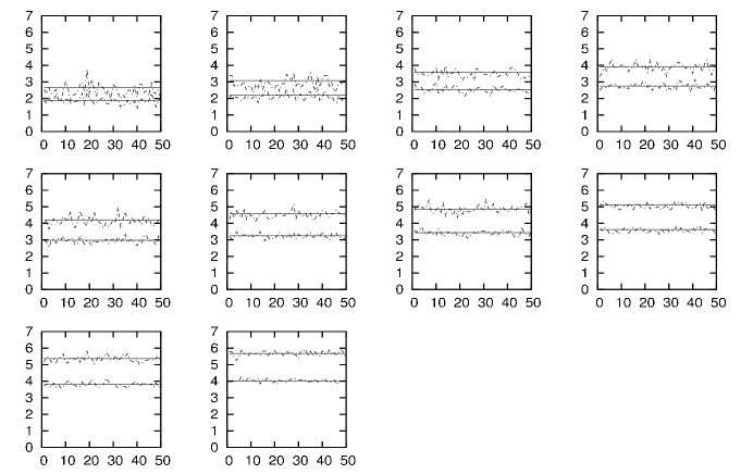
Figure 8: Comparing the expected maxima and difference maxima for $\sigma=1$, from top left corner N=10,20,50,100,200,500,1000,2000,4000,10000. The lower comparision is of $X_{mx}$ and the upper comparision is of $D_{mx}$. The straight line is that calculated theoretically using equations given here (12) & (28), while those obtained from octave(’randn’ function) are the broken lines. Each value is an average of 5 maxima samples. The abscissa is the trial number.

In the fig-7, x1 & x2 are fixed such that the difference between them is d. x3 is allowed to take any value such that the its magnitude of difference with x2 does not exceed d. Next the same is repeated to account the other possibility of x2 and x3 being fixed and x1 being free to take variable values. The net probability would be integrating over x2 from $-\infty$ to $+\infty$ . So we can write this net probability density as,

$$p_{3_{2}}(d)=\frac{2\cdot 2}{(\sigma\sqrt{2\pi})^{3}}\!\!\int_{-\infty}^{+\infty}\ e^{-\frac{x^{2}+(x+d)^{2}}{2\sigma^{2}}}\!\!\int_{-d}^{+d}\ e^{\frac{-(x+y)^{2}}{2\sigma^{2}}}{{d}}y\ \ {{d}}x$$ (21)

$$p_{3_{2}}(d)=\frac{1}{\pi\sigma^{2}}\!\!\int_{-\infty}^{+\infty}\ e^{-\frac{x^{2}+(x+d)^{2}}{2\sigma^{2}}}\left(erf\left(\frac{d+x}{\sigma\sqrt{2}}\right)+erf\left(\frac{d-x}{\sigma\sqrt{2}}\right)\right)\ \ {{d}}x$$ (22)

The factor of 2 in the numerator is due to the fact that d in the first integrand takes 2 values +ve and -ve and in both the cases it integrates to the same amount. Another 2 is due to the interchange of roles between x1 and x3. Now when a similar analysis is done by considering 4 channels and taking the difference in two channels independently, we see that the probabilities are approximately same for occurence of a difference d in the two cases. The probability in the case of 4 channels, but pair wise is

$$p_{4_{2}}(d)=\frac{2\cdot 2}{(\sigma\sqrt{2\pi})^{2}}\!\!\int_{-\infty}^{+\infty}\ e^{\frac{-x^{2}+(x+d)^{2}}{2\sigma^{2}}}\!\!\int_{-d}^{+d}p_{2}(y)\ {{d}}y\ {{d}}x$$ (23)

$$p_{4_{2}}(d)=\frac{2}{\pi\sigma^{2}}\!\!\int_{-\infty}^{+\infty}\ e^{\frac{-x^{2}+(x+d)^{2}}{2\sigma^{2}}}erf\left(\frac{d}{2\sigma}\right)\ {{d}}x=\frac{2}{\sigma\sqrt{\pi}}\ e^{-\frac{d^{2}}{4\sigma^{2}}}\ erf\left(\frac{d}{2\sigma}\right)$$ (24)

This calculation can also be done by applying $p_{2}(d)$ to both pairs. It can be checked(here checked numerically) that for a given value of d,

$$p_{3_{2}}\approx p_{4_{2}}$$ (25)

Hence one can assume that the channels behave approximately independently pair wise in a series of N channels. By considering the difference probability distribution for 2 channels and treating the N-1 channel pairs as new single channels in which the occurence value is not ’x’ but ’d’ we can write using the same derivation as for $X_{mx}$ for the maximum expected difference value in a N channel gaussian noise as,

$$\left<D_{mx}\right>=\frac{N-1}{\sigma\sqrt{\pi}}\!\!\int_{0}^{\infty}\ d\ e^{-\frac{d^{2}}{4\sigma^{2}}}\left[erf\left(\frac{d}{2\sigma}\right)\right]^{N-2}{{d}}d$$ (26)

which again using $S=\left[erf\left(\frac{d}{2\sigma}\right)\right]^{N-1}$ can be written as,

$$\left<D_{mx}\right>=2\sigma\!\!\int_{0}^{1}erf^{-1}\left(S^{\frac{1}{N-1}}\right){{d}}S$$ (27)

For large N the -1 in the exponent can be dropped and simply one can use from (11)

$$\left<D_{mx}\right>=\sqrt{2}\left<X_{mx}\right>$$ (28)

The derivations given here are of the author. He is unaware of any such derivations or results.

Figure 9: The results obtained using difference and added difference methods on spectral line observations at  328 MHz using Ooty Radio Telescope(ORT) towards 4 Galactic positions, inset left. WAE -collapse with automated editing and baseline removal, AD - collapse of actual data. The right plots are the auto-edited versions of the left plots. Interference detection & editing was performed on 10-sec data. The collapse on the right consists of hundreds of such spectra. During editing the interference infected channels were replaced by noise of the same standard deviation as in the reference block + a straight line connecting adjacent channels on the two sides of the interference line.

Figure 10: Noise sampled from a large collection(ORT-100, WSRT-23) of Ton/Toff - 1 after baseline removal(refer fig-1). For ORT Ton and Toff correspond to 1-second spectrum, where as for WSRT its 1-minute.

References

- [1] K.Rohlfs & T.L.Wilson, Tools of Radio Astronomy (A & A Library), Chapter-4