On the hydrodynamical limit for a one dimensional
kinetic model of cell aggregation by chemotaxis

François James  and  Nicolas Vauchelet

1 Introduction

1.1 Modeling

Chemotaxis is a process in which a population of cells rearrange its structures, reacting to the presence of a chemical substance in the environment. In the case of positive chemotaxis, cells migrate towards a concentration gradient of chemoattractant, allowing them to aggregate. Since several years, many attemps for describing chemotaxis from a Partial Differential Equations viewpoint have been considered. The population at the macroscopic level is described by a coupled system on its density and the chemoattractant concentration. The most famous Patlak, Keller and Segel model [18, 23] is formed of parabolic or elliptic equations coupled through a drift term. Although this model has been successfully used to describe aggregation of cells, this macroscopic model has several shortcomings, for instance the detailed individual movement of cells is not taken into account.

In the 80’s, experimental observations have shown that the motion of bacteria (e.g. Escherichia Coli) is due to the alternance of ‘runs and tumbles’ [1, 14, 20, 22]. Therefore kinetic approaches for chemotaxis have been proposed. The so-called Othmer-Dunbar-Alt model [20, 22, 24] describes the dynamic of the distribution function $f$ of cells at time $t$, position $x$ and velocity $v$ and of the concentration of chemoattractant $S$ :

$$\left\{\begin{array}[]{l}\displaystyle\partial_{t}f+v\cdot\nabla_{x}f=\int_{v^{\prime}\in V}(T[S](v^{\prime}\to v)f(v^{\prime})-T[S](v\to v^{\prime})f(v))\,dv^{\prime},\\ \displaystyle-\Delta S+S=\rho(t,x):=\int_{v\in V}f(t,x,v)\,dv.\end{array}\right.$$ (1)

In this equation, $V$ is the set of admissible velocities. The turning kernel $T[S](v^{\prime}\to v)$ denotes the probability of cells to change their velocity from $v^{\prime}$ to $v$. Several works have been devoted to the mathematical study of this kinetic system, under various assumptions on the turning kernel, see for instance [11, 10, 13, 17]. Here we shall assume that the velocities of cells have the same modulus $c$, so that $V=\SS_{c}:=\{v\mid\|v\|=c\}$.

Derivation of macroscopic models from (1) has been investigated by several authors. When the chemotactic orientation, or taxis, that is the weight of the turning kernel, is small compared to the unbiased movement of cells, the limit equations are of diffusion or drift-diffusion type. In [16, 21], the authors show that the Patlak-Keller-Segel model can be obtained as a diffusive limit for a given smooth chemoattractant concentration. A rigorous proof for the case of a nonlinear coupling to an equation for the chemical can be found in [11], leading to a drift-diffusion equation.

In this paper we focus on the opposite case, where taxis instead of undirected movement is dominating. The model has been proposed in [12], and we briefly recall how it is obtained. The limit problem is usually of hyperbolic type, see for instance [15]. Dominant taxis is reflected in the transport model by the fact that the dominating part of the turning kernel depends on the gradient of the chemoattractant. At this stage, two possible models are encountered. On the one hand, we can assume that cells are able to compare the present chemical concentrations to previous ones and thus to respond to temporal gradients along their paths. The decision to change direction and turn or to continue moving depends then on the concentration profile of the chemical $S$ along the trajectories of cells. Thus the turning kernel takes the form (independant on $v$)

$$T[S](v^{\prime}\to v)=\phi(\partial_{t}S+v^{\prime}\cdot\nabla_{x}S).$$ (2)

On the other hand, if cells are large enough, it can be assumed that they are able to sense the gradient of the chemoattractant instantly so that we can use instead the expression

$$T[S](v^{\prime}\to v)=\phi(v^{\prime}\cdot\nabla_{x}S).$$ (3)

Theoretical results as well as numerical simulations for models (1)–(2) and (1)–(3) are proposed in [27].

The function $\phi$ in the preceding formulæ is the turning rate, obviously it has to be positive and monotone. More precisely, for attractive chemotaxis, the turning rate is smaller if cells swim in a favorable direction, that is $\partial_{t}S+v^{\prime}\cdot\nabla_{x}S\geq 0$ (or $v\cdot\nabla_{x}S\geq 0$). Thus $\phi$ should be a nonincreasing function. The converse holds true for repulsive chemotaxis. A simplified model for this phenomenon is the following choice for $\phi$: we fix a positive parameter $\alpha$, and take

$$\phi\in C^{\infty}(\mathbb{R}),\quad\phi^{\prime}\leq 0,\quad\phi(x)=\left\{\begin{array}[]{ll}\phi_{0}&\quad\mbox{ if }x<-\alpha,\\ \phi_{0}/4&\quad\mbox{ if }x>\alpha,\\ \end{array}\right.$$ (4)

where $\phi_{0}$ is a given constant. Moreover, for the sake of clarity of the paper, we will assume the following symmetry on $\phi$: there exists an odd function $\widetilde{\phi}$ such that

$$\phi(x)=\phi_{0}\big{(}\frac{5}{8}+\widetilde{\phi}(x)\big{)},\quad\mbox{ and }\quad\widetilde{\phi}(-x)=-\widetilde{\phi}(x).$$ (5)

The turning kernel (2), compared to (3), makes drastic changes in the behaviour of the solutions to the kinetic model (see [27]). Up to now we cannot take it into account in the theory, so that we focus in the following on the expression (3). As observed above, this can be considered as a biologically relevant model.

In the turning kernel, a specific parameter quantifies the “memory” of the bacteria. When this parameter is small, a specific asymptotic regime leads to a macroscopic, hydrodynamic model. In order to introduce this parameter, we rescale the system (1) by setting

$$\begin{array}[]{c}\displaystyle x=x_{0}{\overline{x}},\qquad t=t_{0}{\overline{t}},\qquad v=v_{0}{\overline{v}},\\[5.69054pt] \displaystyle S(t,x)=S_{0}{\overline{S}}({\overline{t}},{\overline{x}}),\qquad f(t,x,v)=f_{0}{\overline{f}}({\overline{t}},{\overline{x}},{\overline{v}}),\qquad\phi(z)=\phi_{0}{\overline{\phi}}(z),\end{array}$$

where $\phi_{0}$ is the typical value for the size of the turning kernel, $v_{0}=c$ is the typical speed, $x_{0}=L_{x}$ is the characteristic length of the device and the typical time is defined by $t_{0}=x_{0}/v_{0}$. Dropping the bars, the scaled version of (1) reads

$$\begin{array}[]{c}\displaystyle\partial_{t}f+v\cdot\nabla_{x}f=\frac{1}{\varepsilon}\int_{V}\left(T[S](v^{\prime}\to v)f(v^{\prime})-T[S](v\to v^{\prime})f(v)\right)\,dv^{\prime},\\[5.69054pt] -\Delta S+S=\rho,\end{array}$$ (6)

where $\displaystyle\varepsilon=\frac{v_{0}}{\phi_{0}x_{0}}\ll 1$ is the parameter we are interested in: it corresponds to the time interval of information sampling for the bacteria. The hydrodynamic limit corresponds to $\epsilon\to 0$, and we first recall formally how it is obtained.

1.2 Formal hydrodynamic limit

We focus in this work on the one dimensional version of (6), so that the transport takes place in $x\in\mathbb{R}$ and the set of velocity is $V=\{-c,c\}$. The expression of the turning kernel simplifies in such a way that (6) with (3) rewrites

$$\partial_{t}f_{\varepsilon}+v\partial_{x}f_{\varepsilon}=\frac{1}{\varepsilon}(\phi(-v\partial_{x}S_{\varepsilon})f_{\varepsilon}(-v)-\phi(v\partial_{x}S_{\varepsilon})f_{\varepsilon}(v)),\qquad v\in V.$$ (7)

$$-\partial_{xx}S_{\varepsilon}+S_{\varepsilon}=\rho_{\varepsilon}=f_{\varepsilon}(v)+f_{\varepsilon}(-v).$$ (8)

We formally let $\varepsilon$ go to $0$ assuming that $S$ and $f$ admit a Hilbert expansion

$$f_{\varepsilon}=f_{0}+\varepsilon f_{1}+\cdots,\qquad S_{\varepsilon}=S_{0}+\varepsilon S_{1}+\cdots$$

Multiplying (7) by $\varepsilon$ and taking $\varepsilon=0$, we find

$$\phi(-c\partial_{x}S_{0})f_{0}(-c)=\phi(c\partial_{x}S_{0})f_{0}(c).$$ (9)

Summing equations $\eqref{cin1D}$ for $c$ and $-c$, we obtain :

$$\partial_{t}(f_{\varepsilon}(c)+f_{\varepsilon}(-c))+c\partial_{x}(f_{\varepsilon}(c)-f_{\varepsilon}(-c))=0.$$ (10)

Moreover, from equation (9) we deduce that

$$f_{0}(c)-f_{0}(-c)=\frac{\phi(-c\partial_{x}S_{0})-\phi(c\partial_{x}S_{0})}{\phi(-c\partial_{x}S_{0})+\phi(c\partial_{x}S_{0})}(f_{0}(c)+f_{0}(-c))$$

The density at equilibrium is defined by $\rho:=f_{0}(c)+f_{0}(-c)=\int f_{0}(v)\,dv$. Taking $\varepsilon=0$ in (10) we finally obtain

$$\partial_{t}\rho+\partial_{x}(a(\partial_{x}S_{0})\rho)=0,$$

where $a$ is defined by

$$a(\partial_{x}S_{0})=c\,\frac{\phi(-c\partial_{x}S_{0})-\phi(c\partial_{x}S_{0})}{\phi(-c\partial_{x}S_{0})+\phi(c\partial_{x}S_{0})}=\frac{4}{5}c\,(\phi(-c\partial_{x}S_{0})-\phi(c\partial_{x}S_{0})),$$

and we have used (5) for the last identity. Notice that $a$ is actually a macroscopic quantity, since we can rewrite

$$a(\partial_{x}S_{0})=-\frac{4}{5}\int_{V}v\,\phi(v\partial_{x}S_{0})\,dv,$$

so that this expression is independant of the sign of $c$.

We couple this equation with the limit of the elliptic problem (8) for the chemoattractant concentration, so that, in summary, and dropping the index $0$, the formal hydrodynamic limit is the following system

$$\displaystyle\partial_{t}\rho+\partial_{x}(a(\partial_{x}S)\rho)=0,$$ (11)

$$\displaystyle a(\partial_{x}S)=\frac{4}{5}c\,(\phi(-c\partial_{x}S)-\phi(c\partial_{x}S)),$$ (12)

$$\displaystyle-\partial_{xx}S+S=\rho,$$ (13)

complemented with the boundary conditions

$$\rho(t=0,x)=\rho^{ini}(x),\qquad\lim_{x\to\pm\infty}\rho(t,x)=0,\qquad\lim_{x\to\pm\infty}S(t,x)=0.$$ (14)

The formal hydrodynamic limit from (7)–(8) to (11)–(12)–(13) has been obtained in [12] and proved rigorously in the two-dimensional setting for a given smooth $S$. The aim of this paper is to give an account of the problems and open questions arising in the study of the whole coupled system.

1.3 Preliminary remarks

First notice that, even in this one dimensional framework, this study leads to difficulties mainly due to the lack of uniform estimates for the solutions to the kinetic model when $\varepsilon$ goes to zero and consequently to the very weak regularity of the solutions to the limit problem. Even though existence of weak solutions to the kinetic model is ensured in a $L^{p}$ setting, no uniform $L^{\infty}$ bounds can be expected. The reader is referred to [27] for some numerical evidences of this phenomenon, which is the mathematical translation of the concentration of bacteria. This is some kind of “blow-up in infinite time”, which for $\varepsilon=0$ leads to actual blow-up in finite time, and creation of Dirac masses. Moreover the balanced distribution vanishing the right hand side of (7) depends on $S_{\varepsilon}$; thus the techniques developed e.g. in [11] cannot be applied.

We turn now to formal considerations about the limit system, noticing on the one hand that a solution of (13) has the explicit expression

$$S(t,x)=K*\rho(t,.)(x),\quad\mbox{where }K(x)=\frac{1}{2}e^{-|x|},$$ (15)

so that the macroscopic conservation equation for $\rho$ (11) can be rewritten

$$\partial_{t}\rho+\partial_{x}(a(\partial_{x}K*\rho)\rho)=0.$$ (16)

When $a$ is the identity function, this is exactly the so-called aggregation equation, which has been studied by several authors, see [2, 3, 4, 19] and references therein. In particular, finite time blow-up is evidenced when the kernel $K$ is not smooth enough.

On the other hand, taking $\alpha=0$ in the definition of $\phi$ (4) and assuming that the chemoattractant concentration is increasing for $x<x_{0}$ and decreasing for $x>x_{0}$ (which is usually true when cells aggregate at the position $x_{0}$), we deduce that $\displaystyle a(\partial_{x}S)=-\frac{3}{5}c\mbox{ sgn}(x-x_{0})$ which presents a singularity at $x=x_{0}$. The conservation equation (11) becomes therefore a linear conservation equation with a discontinuous compressive velocity field, and it is well known that the solution is a Dirac mass. If $\alpha$ is positive, it turns out that a Dirac mass appears as well, after a finite time.

In summary, we have to deal in the limit system with some kind of weakly nonlinear conservation equation on the density $\rho$. Indeed on the one hand the expected velocity field depends on $\rho$, but in a nonlocal way. On the other hand, this equation behaves like linear equations with discontinuous coefficients, in the sense that it admits measure-valued solutions. Therefore a major difficulty in this study will be to define properly the velocity field $a=a(\partial_{x}S)$ and the product $a\rho$.

The paper is organized as follows. In Section 2 we consider the aggregation-like equation (16), and recall existence and uniqueness results as well as the existence of a finite time for which $L^{\infty}$-weak solutions of (11)–(13) blow up. In Section 3, we investigate the hydrodynamical limit of system (7)–(8) and prove in particular that it gives rise to a somehow natural definition of the flux in the conservation equation. Some numerical simulations illustrating this result are furnished in Section 4. Finally, we end this work with some conclusions and remarks.

2 Aggregation-like equation

In this section, we consider the equation

$$\left\{\begin{array}[]{l}\displaystyle\partial_{t}\rho+\partial_{x}(a(\partial_{x}K*\rho)\rho)=0,\\ \displaystyle\rho(t=0,\cdot)=\rho^{ini}.\end{array}\right.$$ (17)

where $K$ is given by (15). We assume that

$$0<\rho^{ini}\in L^{1}\cap L^{\infty}(\mathbb{R}).$$ (18)

When $a(x)\equiv x$, this equation is the so-called aggregation equation (see e.g. [2, 3, 4, 6, 19]). It is known that for singular $\partial_{x}K$, solutions blow up in finite time. More precisely, we show the blow-up in finite time of $L^{\infty}$ weak solutions. Most of the results presented in this section are obtained thanks to a straightforward adaptation of techniques developed in [2, 3, 6, 19]. Therefore some proofs are not detailed.

2.1 Existence and uniqueness of local $L^{\infty}$-weak solution

We prove in this section the local existence and uniqueness of a solution.

Theorem  2.1.

Let $\rho^{ini}\in L^{1}\cap L^{\infty}(\mathbb{R})$. Then there exists a $T>0$ such that there exists a unique weak solution $\rho$ to (17); moreover $\rho\in C([0,T];L^{1}\cap L^{\infty}(\mathbb{R}))$.

The proof is an adaptation of results in [2, 3, 19]. We first recall the definition of the characteristics for this system: $X(s;x,t)$ is a solution of the ODE

$$\frac{dX}{ds}(s;x,t)=a(\partial_{x}K*\rho)(s,X(s)),\qquad X(t;x,t)=x.$$ (19)

Then we have the following representation of the solution of (17):

$$\rho(t,x)=\rho^{ini}(X(0;x,t))\exp\left({-\int_{0}^{t}\partial_{x}a(\partial_{x}K*\rho)(s,X(s-t;x,t))\,ds}\right).$$ (20)

The proof of this theorem relies strongly on the following estimates:

Proposition  2.1.

Let $\rho^{ini}$ such as in (18) and let $\rho$ be a solution of (17) on $[0,T]$. Then there exists $T>0$ such that for all $t\in[0,T]$, there exists a nonnegative constant $C$ such that

$$\|\rho(t,\cdot)\|_{L^{1}(\mathbb{R})}+\|\rho(t,\cdot)\|_{L^{\infty}(\mathbb{R})}\leq C,$$

where $C$ only depends on $\|\rho^{ini}\|_{L^{1}(\mathbb{R})}$ and $\|\rho^{ini}\|_{L^{\infty}(\mathbb{R})}$.

Proof.  The $L^{1}$ estimate is an easy consequence of the mass conservation. Then,

$$|\partial_{t}\rho+a(\partial_{x}K*\rho)\partial_{x}\rho|=|-\partial_{x}(a(\partial_{x}K*\rho))\rho|\leq 2\|a^{\prime}\|_{\infty}|\rho|^{2}.$$

Integrating along the characteristics curves, we get

$$\|\rho(t,\cdot)\|_{L^{\infty}}\leq\|\rho^{ini}\|_{L^{\infty}}+2\|a^{\prime}\|_{\infty}\int_{0}^{t}\|\rho(s,\cdot)\|_{L^{\infty}}^{2}\,ds.$$

We deduce that as long as $2\|a^{\prime}\|_{\infty}\|\rho^{ini}\|_{L^{\infty}}t<1$,

$$\|\rho(t,\cdot)\|_{L^{\infty}}\leq\frac{\|\rho^{ini}\|_{L^{\infty}}}{1-2\|a^{\prime}\|_{\infty}\|\rho^{ini}\|_{L^{\infty}}t}.$$

We notice that $T$ should satisfies the bound $T<1/(2\|a^{\prime}\|_{\infty}\|\rho^{ini}\|_{L^{\infty}})$. $\square$

Proof of existence.  We do not detail the proof of the existence of solution which can be deduced thanks to an adaptation of [2, 3, 19], where the study of an aggregation equation is proposed. We just recall the main argument of the proof in the following steps :

1. We construct a family of approximating solutions $(\rho_{\varepsilon})$ by solving (17) with initial data $\rho^{ini}*g_{\varepsilon}$ where $g_{\varepsilon}$ is a mollifier.

2. We state uniform Lipschitz estimates in space and time on the sequences $(a(\partial_{x}K*\rho_{\varepsilon}))_{\varepsilon}$ and $(X_{\varepsilon})_{\varepsilon}$ and use the Arzelà-Ascoli Theorem to extract converging subsequence.

3. We pass to the limit in the representation (20). $\square$
   

Proof of uniqueness.  The idea of this proof is to use the quantity $S$. Since this idea will be developed for measure-valued solutions, we detail this proof. Computations are done for regular solutions, nevertheless they can be made rigorous by introducing a regularization and passing to the limit (see [2]). Let us consider two classical solutions $\rho_{1}$ and $\rho_{2}$. Denoting $a_{i}=a(\partial_{x}K*\rho_{i})$ for $i=1,2$, we have

$$\partial_{t}(\rho_{1}-\rho_{2})+\partial_{x}(a_{1}(\rho_{1}-\rho_{2}))+\partial_{x}(\rho_{2}(a_{1}-a_{2}))=0.$$ (21)

Define $S(t,x):=(\partial_{x}K*(\rho_{1}-\rho_{2})(t,\cdot))(x)$ which solves the problem

$$-\partial_{xx}S+S=\rho_{1}-\rho_{2},\quad\mbox{ on }\mathbb{R}.$$ (22)

We notice that when $t=0$, we have $S(0,x)=0$. From the weak formulation of equation (21) with the test function $S$, we have

$$\int_{0}^{t}\int_{\mathbb{R}}\partial_{t}(\rho_{1}-\rho_{2})S\,dxds=I+II$$ (23)

where

$$\begin{array}[]{l}\displaystyle I=\int_{0}^{t}\int_{\mathbb{R}}a_{1}(\rho_{1}-\rho_{2})S\,dxds,\\[8.53581pt] \displaystyle II=\int_{0}^{t}\int_{\mathbb{R}}\rho_{2}(a_{1}-a_{2})S\,dxds.\end{array}$$

For the term $I$, we have using (22) and integration by parts

$$I=\int_{0}^{t}\int_{\mathbb{R}}a_{1}(-\partial_{xx}S+S)\,S\,dxds=\frac{1}{2}\int_{0}^{t}\int_{\mathbb{R}}\partial_{x}a_{1}\,|\partial_{x}S|^{2}\,dxds+\int_{0}^{t}\int_{\mathbb{R}}a_{1}S^{2}\,dxds,$$

Moreover,

$$\partial_{x}a_{1}=-\frac{4}{5}c(\phi^{\prime}(-c\partial_{x}S_{1})+\phi^{\prime}(c\partial_{x}S_{1}))\partial_{xx}S_{1}\leq\max\{\frac{8}{5}c\|\phi^{\prime}\|_{L^{\infty}}S_{1},0\},$$

where we use the fact that $\phi$ is a nonincreasing positive function. From the $L^{\infty}$-bound on $S_{1}$, we deduce that there exists $\beta\in L^{1}([0,T])$ such that $\partial_{x}a_{1}\leq\beta$. Thus

$$I\leq\frac{1}{2}\int_{0}^{t}\beta(s)\int_{\mathbb{R}}|\partial_{x}S|^{2}\,dxds+\int_{0}^{t}\int_{\mathbb{R}}a_{1}S^{2}\,dxds.$$

Then, the estimate $|a_{1}|\leq\frac{3}{5}c$ gives

$$I\leq\frac{1}{2}\int_{0}^{t}\beta(s)\|\partial_{x}S\|^{2}_{L^{2}}\,ds+\frac{3}{5}c\int_{0}^{t}\|S\|_{L^{2}}^{2}\,ds.$$ (24)

For the term II of (23), we have thanks to the Cauchy-Schwarz inequality

$$\begin{array}[]{ll}\displaystyle|II|=&\displaystyle\left|\int_{0}^{t}\int_{\mathbb{R}}\rho_{2}(a(\partial_{x}K*\rho_{1})-a(\partial_{x}K*\rho_{2}))S\,dxds\right|\\[5.69054pt] &\displaystyle\leq\int_{0}^{t}\|\rho_{2}\|_{L^{\infty}}\|a^{\prime}\|_{\infty}\|\partial_{x}K*(\rho_{1}-\rho_{2})\|_{L^{2}}\|S\|_{L^{2}}\,ds.\end{array}$$

Since $\partial_{x}S=\partial_{x}K*(\rho_{1}-\rho_{2})$, we obtain

$$|II|\leq\frac{1}{2}\int_{0}^{t}\|\rho_{2}\|_{L^{\infty}}\|a^{\prime}\|_{\infty}(\|\partial_{x}S\|_{L^{2}}^{2}+\|S\|_{L^{2}}^{2})\,ds.$$ (25)

Then, we notice that using (22) and thanks to an integration by parts the left hand side of (23) can be rewritten

$$\int_{0}^{t}\int_{\mathbb{R}}\partial_{t}(\rho_{1}-\rho_{2})S\,dxds=\frac{1}{2}\int_{\mathbb{R}}(|\partial_{x}S|^{2}+S^{2})\,dx$$ (26)

Finally, we deduce from (23), (24), (25) and (26),

$$\int_{\mathbb{R}}(|\partial_{x}S|^{2}+S^{2})\,dx\leq\int_{0}^{t}\|\rho_{2}\|_{L^{\infty}}\|a^{\prime}\|_{\infty}\left(\beta(s)\|\partial_{x}S\|_{L^{2}}^{2}+\frac{3}{5}c\|S\|_{L^{2}}^{2}\right)\,ds.$$

Uniqueness follows from a Gronwall type argument. $\square$

2.2 Blow-up in finite time

The blow-up of solutions of a one dimensional aggregation solution is proposed for instance in [6] where it is proved by the method of characteristics that aggregation of mass occurs. In [2, 3], the finite time blow-up is obtained thanks to an energy estimate. We assume that the initial data is given symmetric with respect to $0$ and positive. It is easy to show then that for all $t>0$, $\rho(t,x)=\rho(t,-x)$. Moreover, for the sake of simplicity, we assume that there exists $\delta>0$ such that supp$(\rho^{ini})\subset[-\delta,\delta]$. Then for all $x>\delta$ the function $S^{ini}=K*\rho^{ini}$ satisfies $\partial_{x}S^{ini}(x)<0$, so that the characteristics defined by (19) are inward. Thus for all $t>0$, supp$(\rho(t,\cdot))\subset[-\delta,\delta]$.

The energy of the system is defined as

$$E(t)=\frac{1}{2}\int_{\mathbb{R}}(|\partial_{x}S|^{2}+|S|^{2})\,dx=\frac{1}{2}\int_{\mathbb{R}}\rho S\,dx,$$ (27)

where the last formulation is obtained by integration by parts. On the one hand, we have the obvious bound

$$E(t)\leq\frac{1}{2}\|\rho\|_{L^{1}}\|K*\rho\|_{L^{\infty}}\leq\frac{1}{2}\|\rho\|_{L^{1}}^{2}.$$ (28)

On the other hand, using (17) we have

$$\frac{d}{dt}E(t)=\int_{\mathbb{R}}a(\partial_{x}S)\partial_{x}S\rho\,dx.$$

Moreover $\|\partial_{x}S\|_{L^{\infty}}\leq\frac{1}{2}\|\rho^{ini}\|_{L^{1}}$. Since the function $a$ is assumed to be regular, there exists $\zeta>0$ such that $a(x)x\geq\zeta|x|^{2}$ for all $x\in[-\frac{1}{2}\|\rho^{ini}\|_{L^{1}},\frac{1}{2}\|\rho^{ini}\|_{L^{1}}]$. Thus,

$$\frac{d}{dt}E(t)\geq\zeta\int_{\mathbb{R}}|\partial_{x}S|^{2}\rho\,dx.$$ (29)

We now make use of the following result whose proof is given in [3]:

Proposition  2.2.

There exists a constant $C>0$ such that for all $\delta$ sufficiently small, we have for any symmetric nonnegative function $\rho$ in $L^{1}(\mathbb{R})$ with a compact support in $[-\delta,\delta]$,

$$\int_{\mathbb{R}}|\partial_{x}K*\rho|^{2}\rho\,dx\geq C.$$

Then, from (29) there exists a constant $C>0$ such that for all $t>0$,

$$E(t)-E(0)\geq Ct.$$

Therefore, with (28) we have proved

Theorem  2.2.

Let $\rho$ be a symmetric solution of (17) with symmetric, positive initial data with compact support included in $[-\delta,\delta]$. For sufficiently small $\delta$, there exists a time $T^{*}>0$ for which the solution $\rho$ ceases to exist, i.e.

$$\lim_{t\to T^{*}}\|\rho(t,.)\|_{L^{p}(\mathbb{R})}=+\infty,\quad\mbox{ for }p\in(1,\infty).$$

3 Convergence for the kinetic model

In this section we investigate the convergence of a sequence of solutions to the microscopic model (7)–(8). We are not able yet to obtain rigorously (11)–(13). We actually prove that the whole sequence of solutions is convergent, and that the macroscopic density satisfies a conservation equation with a uniquely determined flux. More precisely, the main result of this section is the following theorem. We introduce the macroscopic densities

$$\rho_{\varepsilon}=\int_{V}f_{\varepsilon}\,dv,\qquad\rho=\int_{V}f\,dv.$$

Theorem  3.1.

Let $T>0$ and let us assume that $\rho^{ini}$ is given in ${\cal M}_{b}(\mathbb{R})$. Let $(f_{\varepsilon},S_{\varepsilon})$ be a solution to the kinetic–elliptic equation (7)–(8) with initial data $f_{\varepsilon}^{ini}$ such that $\rho_{\varepsilon}^{ini}:=\int_{V}f_{\varepsilon}^{ini}\,dv=\eta_{\varepsilon}*\rho^{ini}$ where $\eta_{\varepsilon}$ is a mollifier. Then as $\varepsilon\to 0$, the sequence converges to $(\rho,S)$ in the following sense :

$$\begin{array}[]{c}\displaystyle\rho_{\varepsilon}\rightharpoonup\rho\qquad\mbox{ in }\quad{\cal S}_{\cal M}:=C([0,T];{\cal M}_{b}(\mathbb{R})-\sigma({\cal M}_{b},C_{0})),\\[5.69054pt] \displaystyle S_{\varepsilon}\rightharpoonup S\qquad\mbox{ in }\quad C([0,T];W^{1,\infty}(\mathbb{R}))-weak,\end{array}$$

and $(\rho,S)$ is the unique solution in the distribution sense of

$$\left\{\begin{array}[]{l}\displaystyle\partial_{t}\rho+\partial_{x}J=0,\\[5.69054pt] \displaystyle-\partial_{xx}S+S=\rho,\end{array}\right.$$ (30)

complemented with initial data $\rho^{ini}$ and where

$$J=-\partial_{x}(A(\partial_{x}S))+a(\partial_{x}S)S\quad\mbox{ a.e. }$$

Before turning to the proof of this result we notice that the problem (30) is equivalent to

$$\partial_{t}S-\partial_{x}K*\left[\partial_{x}(A(\partial_{x}S))+a(\partial_{x}S)S\right]=0,\quad\mbox{ in }{\cal D}^{\prime}(\mathbb{R}).$$ (31)

This is obtained by taking the convolution with $K$ of the first equation in (30). This emphasizes the key role of $S$ in the study of the limit.

3.1 Preliminary results

First we recall the following statement on the kinetic-elliptic problem.

Theorem  3.2.

Let $T>0$ and $\varepsilon>0$. Assume $f_{\varepsilon}^{ini}\in C(\mathbb{R})$. Then problem (7)–(8) complemented with initial data $f_{\varepsilon}^{ini}$ admits a unique weak solution in $C([0,T]\times\mathbb{R}\times V)\times C([0,T];C^{2}(\mathbb{R}))$. Moreover, we have the following estimates uniform in $\varepsilon>0$ :

$$\int_{\mathbb{R}}\int_{V}|v|^{k}f_{\varepsilon}\,dxdv=|v|^{k}|\rho^{ini}|(\mathbb{R})\,,\quad\mbox{ k }\in\mathbb{N}.$$ (32)

Proof.  The proof of the existence can be found in [27]. The estimates (32) rely on the conservation of the mass and on the fact that since $v\in V=\SS_{c}$, $|v|$ is constant. $\square$

Then, we furnish a convergence result for a sequence of functions $S$.

Lemma  3.1.

Let $(\rho_{n})_{n\in\mathbb{N}}$ be a sequence of measures that converges weakly towards $\rho$ in ${\cal S}_{\cal M}$. Let $S_{n}(t,x)=(K*\rho_{n}(t,\cdot))(x)$ and $S(t,x)=(K*\rho(t,\cdot))(x)$, where $K$ is defined in (15). Then when $n\to\infty$ we have

$$\begin{array}[]{rcl}\partial_{x}S_{n}(t,x)&\longrightarrow&\partial_{x}S(t,x)\quad\mbox{ for a.e. }t\in[0,T],\ x\in\mathbb{R},\\ \partial_{x}S_{n}(t,x)&\rightharpoonup&\partial_{x}S(t,x)\quad\mbox{in }L^{\infty}w-*\end{array}$$

Proof.  We have that

$$\partial_{x}S_{n}(t,x)=\big{(}\partial_{x}K*\rho_{n}(t,\cdot)\big{)}(x)=\int_{\mathbb{R}}\frac{1}{2}\frac{x-y}{|x-y|}e^{-|x-y|}\,\rho_{n}(t,dy).$$ (33)

Let $\varepsilon>0$, we regularize the convolution kernel by introducing the following functions :

$$\phi_{x,\varepsilon}(y)=\left\{\begin{array}[]{ll}\displaystyle\frac{1}{2}\frac{x-y}{|x-y|}e^{-|x-y|},\qquad\mbox{ on }(-\infty,x-\varepsilon]\cup[x,+\infty),\\ \displaystyle\frac{1}{2}\left(\frac{1+e^{-\varepsilon}}{\varepsilon}(y-x)+1\right),\qquad\mbox{ on }(x-\varepsilon,x).\\ \end{array}\right.$$

$$\psi_{x,\varepsilon}(y)=\left\{\begin{array}[]{ll}\displaystyle\frac{1}{2}\frac{x-y}{|x-y|}e^{-|x-y|},\qquad\mbox{ on }(-\infty,x]\cup[x+\varepsilon,+\infty),\\[5.69054pt] \displaystyle\frac{1}{2}\left(\frac{1+e^{-\varepsilon}}{\varepsilon}(y-x)-1\right),\qquad\mbox{ on }(x,x+\varepsilon).\\[5.69054pt] \end{array}\right.$$

With this definition, we clearly have for all $x$, $y$ in $\mathbb{R}$

$$\psi_{x,\varepsilon}(y)\leq\frac{1}{2}\frac{x-y}{|x-y|}e^{-|x-y|}\leq\phi_{x,\varepsilon}(y).$$ (34)

Moreover by definition of the weak convergence,

$$\lim_{n\to+\infty}\int_{\mathbb{R}}\phi_{x,\varepsilon}(y)\,\rho_{n}(t,dy)=\int_{\mathbb{R}}\phi_{x,\varepsilon}(y)\,\rho(t,dy).$$

Then, from (33) and (34), we deduce

$$\limsup_{n\to+\infty}\partial_{x}S_{n}\leq\int_{\mathbb{R}}\phi_{x,\varepsilon}(y)\,\rho(t,dy).$$

Moreover,

$$\begin{array}[]{ll}\displaystyle\int_{\mathbb{R}}\phi_{x,\varepsilon}(y)\,\rho(t,dy)&\displaystyle=\partial_{x}S+\frac{1}{2}\int_{x-\varepsilon}^{x}\left(1+\frac{1+e^{-\varepsilon}}{\varepsilon}(y-x)-e^{y-x}\right)\,\rho(t,dy)\\[8.53581pt] &\displaystyle\leq\partial_{x}S+\frac{1}{2}(1-e^{-\varepsilon})|\rho(t,\cdot)|(\mathbb{R})\end{array}$$

By the same token with $\psi_{x,\varepsilon}$, we obtain the estimate

$$\begin{array}[]{ll}\displaystyle\partial_{x}S-\frac{1}{2}(1-e^{-\varepsilon})|\rho(t,\cdot)|(\mathbb{R})&\displaystyle\leq\liminf_{n\to+\infty}\partial_{x}S_{n}\\[5.69054pt] &\displaystyle\leq\limsup_{n\to+\infty}\partial_{x}S_{n}\leq\partial_{x}S+\frac{1}{2}(1-e^{-\varepsilon})|\rho(t,\cdot)|(\mathbb{R}).\end{array}$$

Letting $\varepsilon\to 0$, we get $\lim_{n\to+\infty}\partial_{x}S_{n}(t,x)=\partial_{x}S(t,x)$ for almost all $t\in[0,T]$ and $x\in\mathbb{R}$. $\square$
We turn now to the uniqueness of $S$, which is the key point to get the uniqueness result in Theorem 3.1.

3.2 Uniqueness for $S$

In [2] (see proof of Theorem 2.1 too), the authors obtain the uniqueness on the aggregation equation by introducing a quantity which appears here naturally to be the potential $S$. They get an estimate that relies strongly on the $L^{\infty}$ bound on the density whereas here it is only measure-valued with a finite total variation. Therefore, we have to work in a weaker space, and we use the fact that the function $S$ defined by $S=K*\rho$ is a weak solution of (31). We have the following result.

Proposition  3.1.

Let $S_{1}$ and $S_{2}$ be two weak solutions of (31) in $L^{\infty}([0,T];B(\mathbb{R}))\cap C([0,T];W^{1,1}(\mathbb{R}))$ with initial data $S_{1}^{ini}$ and $S_{2}^{ini}$ respectively. Then there exists a nonnegative constant $C$ such that

$$\|S_{1}-S_{2}\|_{L^{\infty}([0,T];W^{1,1}(\mathbb{R}))}\leq C\|S_{1}^{ini}-S_{2}^{ini}\|_{W^{1,1}(\mathbb{R})}.$$

Proof.  We introduce a function $A\in C^{\infty}(\mathbb{R})$ such that $A^{\prime}=a$. Now, differentiating (31) and noticing that $K$ satisfies $-\partial_{xx}K+K=\delta_{0}$, we get

$$\partial_{t}\partial_{x}S+\partial_{x}(A(\partial_{x}S))-\partial_{x}K*A(\partial_{x}S)+K*(a(\partial_{x}S)S)-a(\partial_{x}S)S=0.$$ (35)

The definition of $S$, $S(t,x)=(K*\rho(t,\cdot))(x)$, implies that $\partial_{x}S$ belongs to $L^{\infty}(0,T;BV(\mathbb{R}))$. Therefore equations (31)–(35) have a sense in their weak formulation. Let $S_{1}$ and $S_{2}$ satisfy the weak formulations of (31)–(35) with initial data $S_{1}^{ini}$ and $S_{2}^{ini}$ respectively. We denote by $a_{1}=a(\partial_{x}S_{1})$ and $a_{2}=a(\partial_{x}S_{2})$. We deduce from (35) that

$$\begin{array}[]{c}\displaystyle\partial_{t}\partial_{x}(S_{1}-S_{2})+\partial_{x}(A(\partial_{x}S_{1})-A(\partial_{x}S_{2}))=\\[11.38109pt] \displaystyle\partial_{x}K*(A(\partial_{x}S_{1})-A(\partial_{x}S_{2}))+a_{1}S_{1}-a_{2}S_{2}-K*(a_{1}S_{1}-a_{2}S_{2}).\end{array}$$

Multiplying this equation by ${\rm sign}(\partial_{x}(S_{1}-S_{2}))$, integrating with respect to $x$ and using the properties of the convolution product, we deduce

$$\begin{array}[]{ll}\displaystyle\frac{d}{dt}\int_{\mathbb{R}}|\partial_{x}(S_{1}-S_{2})|\,dx\leq&\displaystyle\|\partial_{x}K\|_{\infty}\int_{\mathbb{R}}|A(\partial_{x}S_{1})-A(\partial_{x}S_{2})|\,dx+\\[11.38109pt] &\displaystyle+(1+\|K\|_{\infty})\int_{\mathbb{R}}|a_{1}S_{1}-a_{2}S_{2}|\,dx.\end{array}$$

The function $a$ being regular, we deduce

$$\frac{d}{dt}\int_{\mathbb{R}}|\partial_{x}(S_{1}-S_{2})|\,dx\leq C_{0}\int_{\mathbb{R}}|\partial_{x}(S_{1}-S_{2})|\,dx+C_{1}\int_{\mathbb{R}}|S_{1}-S_{2}|\,dx.$$ (36)

By the same token with equation (31), it leads to

$$\frac{d}{dt}\int_{\mathbb{R}}|S_{1}-S_{2}|\,dx\leq C_{2}\int_{\mathbb{R}}|\partial_{x}(S_{1}-S_{2})|\,dx+C_{3}\int_{\mathbb{R}}|S_{1}-S_{2}|\,dx.$$ (37)

Summing (37) and (36), we deduce that there exists a nonnegative constant $C$ such that

$$\frac{d}{dt}\|S_{1}-S_{2}\|_{W^{1,1}(\mathbb{R})}\leq C\|S_{1}-S_{2}\|_{W^{1,1}(\mathbb{R})}.$$

Applying the Gronwall Lemma allows to conclude the proof. $\square$

3.3 Proof of Theorem 3.1

Let $(f_{\varepsilon},S_{\varepsilon})$ be a solution of (7)–(8). For fixed $\varepsilon>0$, we have $f_{\varepsilon}\in C([0,T]\times\mathbb{R}\times V)$. We define the flux $\displaystyle J_{\varepsilon}:=\int_{V}vf_{\varepsilon}\,dv$ and the macroscopic velocity

$$a(\partial_{x}S_{\varepsilon})=-\frac{\int_{V}v\phi(v\partial_{x}S_{\varepsilon})\,dv}{\int_{V}\phi(v\partial_{x}S_{\varepsilon})\,dv}=\frac{4}{5}v(\phi(-v\partial_{x}S_{\varepsilon})-\phi(v\partial_{x}S_{\varepsilon})).$$

We can rewrite the kinetic equation (7) as

$$\partial_{t}f_{\varepsilon}+v\partial_{x}f_{\varepsilon}=\frac{1}{\varepsilon}(\phi(-v\partial_{x}S_{\varepsilon})\rho_{\varepsilon}-\frac{5}{4}f_{\varepsilon}).$$

Taking the zeroth and first order moments, we get

$$\displaystyle\partial_{t}\rho_{\varepsilon}+\partial_{x}J_{\varepsilon}=0,$$ (38)

$$\displaystyle\partial_{t}J_{\varepsilon}+v^{2}\partial_{x}\rho_{\varepsilon}=\frac{1}{\varepsilon}\frac{5}{4}(a(\partial_{x}S_{\varepsilon})\rho_{\varepsilon}-J_{\varepsilon}).$$ (39)

From (38), we deduce that

$$\forall\,t\in[0,T],\quad|\rho_{\varepsilon}(t,\cdot)|(\mathbb{R})=|\rho^{ini}|(\mathbb{R}).$$

Therefore, for all $t\in[0,T]$ the sequence $(\rho_{\varepsilon}(t,\cdot))_{\varepsilon}$ is relatively compact in ${\cal M}_{b}(\mathbb{R})-\sigma({\cal M}_{b}(\mathbb{R}),C_{0}(\mathbb{R}))$. Moreover, there exists $u_{\varepsilon}\in L^{\infty}([0,T],BV(\mathbb{R}))$ such that $\rho_{\varepsilon}=\partial_{x}u_{\varepsilon}$. From (38), we get that $\partial_{t}u_{\varepsilon}=-J_{\varepsilon}$ and with estimate (32) for $k=1$ we deduce that $u_{\varepsilon}$ is bounded in Lip$([0,T],L^{1}(\mathbb{R}))$. It implies the equicontinuity in $t$ of $(\rho_{\varepsilon})_{\varepsilon}$. Thus the sequence $(\rho_{\varepsilon})_{\varepsilon}$ is relatively compact in ${\cal S}_{\cal M}$ and we can extract a subsequence still denoted $(\rho_{\varepsilon})_{\varepsilon}$ that converges towards $\rho$ in ${\cal S}_{\cal M}$.

We recall that $S_{\varepsilon}(t,x)=(K*\rho_{\varepsilon}(t,\cdot))(x)$ where $K(x)=\frac{1}{2}e^{-|x|}$. Denoting $S(t,x):=(K*\rho(t,\cdot))(x)$, since $\rho\in{\cal S}_{\cal M}$, we have $S\in L^{\infty}([0,T];BV(\mathbb{R}))$. From Lemma 3.1, the sequence $(\partial_{x}S_{\varepsilon})_{\varepsilon}$ converges in $L^{\infty}w-*$ and a.e. to $\partial_{x}S$ as $\varepsilon$ goes to $0$.

From (38)–(39), we have in the distribution sense

$$\partial_{t}\rho_{\varepsilon}+\partial_{x}(a(\partial_{x}S_{\varepsilon})\rho_{\varepsilon})=\partial_{x}(a(\partial_{x}S_{\varepsilon})\rho_{\varepsilon}-J_{\varepsilon})=\frac{4}{5}\varepsilon\partial_{x}(\partial_{t}J_{\varepsilon}+v^{2}\partial_{x}\rho_{\varepsilon})=R_{\varepsilon}.$$ (40)

Now, for all $\psi\in C^{2}_{c}((0,T)\times\mathbb{R})$, we deduce from (32)

$$\left|\int(\partial_{t}J_{\varepsilon}+v^{2}\partial_{x}\rho_{\varepsilon})\partial_{x}\psi\,dxdt\right|\leq|v||\rho^{ini}|(\mathbb{R})\|\partial_{t}\partial_{x}\psi\|_{L^{\infty}}+|v|^{2}|\rho^{ini}|(\mathbb{R})\|\partial_{xx}\psi\|_{L^{\infty}}.$$

This implies that the limit in the distribution sense of the right-hand side $R_{\varepsilon}$ of (40) vanishes.

On the one hand, multiplying equation (8) by $a(\partial_{x}S_{\varepsilon})$ and introducing the real-valued function $A$ such that $A^{\prime}=a$, we get

$$a(\partial_{x}S_{\varepsilon})\rho_{\varepsilon}=-\partial_{x}(A(\partial_{x}S_{\varepsilon}))+a(\partial_{x}S_{\varepsilon})S_{\varepsilon},$$ (41)

so that we can rewrite the conservation equation (40) as follows, in ${\cal D}^{\prime}(\mathbb{R})$ :

$$\partial_{t}\rho_{\varepsilon}+\partial_{x}\left(-\partial_{x}A(\partial_{x}S_{\varepsilon})+a(\partial_{x}S_{\varepsilon})S_{\varepsilon}\right)=\frac{4}{5}\varepsilon\partial_{x}(\partial_{t}J_{\varepsilon}+v^{2}\partial_{x}\rho_{\varepsilon}).$$ (42)

Taking the limit $\varepsilon\to 0$ in the distribution sense of equation (42), we get that in ${\cal D}^{\prime}(\mathbb{R})$

$$\partial_{t}\rho+\partial_{x}\left(-\partial_{x}A(\partial_{x}S)+a(\partial_{x}S)S\right)=0,$$ (43)

where $S(t,x)=(K*\rho(t,\cdot))(x)$. We recall that we have chosen the initial data such that $\rho_{\varepsilon}^{ini}=\eta_{\varepsilon}*\rho^{ini}$ where $\eta_{\varepsilon}$ is a mollifier. Therefore $\rho_{\varepsilon}^{ini}\rightharpoonup\rho^{ini}$ in ${\cal M}_{b}(\mathbb{R})-\sigma({\cal M}_{b}(\mathbb{R}),C_{0}(\mathbb{R}))$.

On the other hand, as noticed above, $S$ satisfies (31) and (35) in the distribution sense. Proposition 3.1 above asserts that $S$ satisfying (31)–(35) is unique. Thus $\rho$ is unique since, if we assume that there exist $\rho_{1}$ and $\rho_{2}$ satisfying (43) in the distribution sense, then by the uniqueness of the solution of (31)–(35), we have that $K*\rho_{1}=K*\rho_{2}$ which implies that $\rho_{1}=\rho_{2}$. Finally, thanks to the uniqueness, all the sequence $\rho_{\varepsilon}$ converges to $\rho$ in ${\cal S}_{\cal M}$.

4 Numerical simulations

We illustrate the previous convergence result with some numerical simulations of the problem (7)–(8). We discretize the kinetic equation thanks to a semi-lagrangian scheme and the elliptic equation for $S$ is discretized with $P_{1}$ finite elements. We refer the reader to [27] for more details on the numerical scheme. Notice that letting $\epsilon$ go to 0 in the simulations is very difficult because of the high numerical diffusivity of the scheme.

We have chosen to present simulations with realistic numerical values. For the bacteria Escherichia Coli the velocity is $c=20.\,10^{-6}$ $m.s^{-1}$ and the density of cells is $n_{0}=10^{11}$ $m^{-1}$. The domain is assumed to be an interval of length $x_{0}=1\,cm$. The turning kernel is given by (3) with $\phi$ in (4). Due to the large value of $n_{0}$, the value of the parameter $\alpha$ should be very large to have an influence; thus this parameter does not play a role in the dynamics of bacteria and for the simulations we have fixed $\alpha=1$. We assume that the initial concentration of cells is a Gaussian centered in the middle of the domain. We run simulations with three different values for $\phi_{0}$ : $\phi_{0}=0.05$, $1$ and $20$ so that $\varepsilon=v_{0}/(\phi_{0}x_{0})$ takes the values $10^{-4}$, $2.\,10^{-3}$ and $4.\,10^{-2}$.

In Figures 1 and 2 we present evolution of the density of cells with respect to the time and to $\varepsilon$. We observe the aggregation of cells in the center of the domain which is the first step of the formation of a Dirac. As $\varepsilon\to 0$, the aggregation phenomenon is faster and the solution seems to converge to a Dirac. We display the evolution of the gradient of the chemoattractant concentration $\partial_{x}S$ in Figures 3 and 4. A singularity in the center of the domain appears clearly.

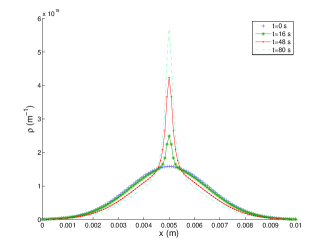
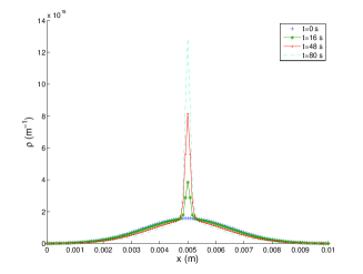
Figure 1: Time evolution of the density $\rho$ of bacteria for different values of the parameters $\varepsilon$. Left : $\varepsilon=4.\,10^{-2}$. Right : $\varepsilon=10^{-4}$.

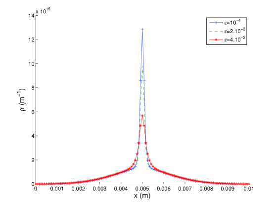
Figure 2: Density $\rho$ of cells for different values of the parameters $\varepsilon$ at time $t=80$ s. As $\varepsilon$ becomes smaller the concentration effect is more important.

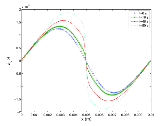
Figure 3: Time dynamics of the gradient of potential $\partial_{x}S$ with $\varepsilon=10^{-4}$. As time increases the derivative of the potential tends to become singular.

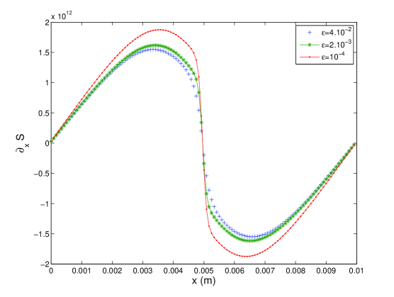
Figure 4: Gradient of the potential $\partial_{x}S$ for different values for $\varepsilon$ at time $t=80~{}$s.

5 Conclusion

In this work we have studied the convergence of a kinetic model of cells aggregation by chemotaxis towards a hydrodynamic model which appears to be a conservation law coupled to an elliptic equation. Although the limit of the macroscopic quantity $\rho_{\varepsilon}$ and $S_{\varepsilon}$ have been obtained in Theorem 3.1, this mathematical result is not completely satisfactory since the limit model (30) does not allow to define a macroscopic velocity for the flux. Formally, this macroscopic velocity is given by $a(\partial_{x}S)$ defined by (12). However, since $\rho$ is only measure-valued, $\partial_{x}S$ belongs to $BV(\mathbb{R})$, hence we cannot give a sense to the product $a(\partial_{x}S)\rho$.

A possible convenient setting to overcome this difficulty is the notion of duality solutions, introduced by Bouchut and James [7]. In this framework, we can solve the Cauchy problem for conservation equations in one dimension with a coefficient $a$ that satisfies a one-sided Lipschitz condition. The theory in higher dimensions is not complete [9], and Poupaud and Rascle [26] (see also[5]) for another approach, which coincides with duality in the 1-d case. It is actually not difficult to prove that $a$ defined in (12) is one-sided Lipschitz. In fact, from $\rho\geq 0$, we deduce that $-\partial_{xx}S\leq S$. After straightforward computation, we get

$$\partial_{x}(a(\partial_{x}S))=-\frac{4}{5}c(\phi^{\prime}(-c\partial_{x}S)+\phi^{\prime}(c\partial_{x}S))\partial_{xx}S.$$

Therefore, $\phi$ being nonincreasing and smooth, we deduce

$$\partial_{x}(a(\partial_{x}S))\leq\max\{\frac{8}{5}c\|\phi^{\prime}\|_{L^{\infty}}S,0\}.$$

And the properties of the convolution lead to

$$\|S(t,\cdot)\|_{L^{\infty}}\leq\frac{1}{2}|\rho(t,\cdot)|(\mathbb{R})=\frac{1}{2}|\rho^{ini}|(\mathbb{R}).$$

Finally, $a$ satisfies the OSL condition :

$$\exists\,\beta\in L^{1}([0,T]),\quad\partial_{x}a(t,\cdot)\leq\beta(t)\quad\mbox{in the distribution sense. }$$

However, we are not able to prove the uniqueness of the duality solutions for the hydrodynamic problem. In fact, the uniqueness proof in Section 3.2 relies on the fact that the potential $S$ satisfies equation (31) and thus on the definition the flux $J$ in (30). In the framework of duality solution, the conservation equation is not a priori satisfied in the distribution sense. A generalized flux that has a priori no link with $J$ in (30) is then introduced. The relation between these flux and therefore the passage from $J$ to the macroscopic velocity $a$ is still an open question.

Acknowledgments.  The authors acknowledge Benoît Perthame for driving their attention on this problem of hydrodynamic limit.

François James
Université d’Orléans, Mathématiques, Applications et Physique Mathématique d’Orléans,
CNRS UMR 6628, MAPMO
Fédération Denis Poisson, CNRS FR 2964,
45067 Orléans cedex 2, France
e-mail: Francois.James@univ-orleans.fr
Nicolas Vauchelet
UPMC Univ Paris 06, UMR 7598, Laboratoire Jacques-Louis Lions,
CNRS, UMR 7598, Laboratoire Jacques-Louis Lions and
INRIA Paris-Rocquencourt, Equipe BANG
F-75005, Paris, France,
e-mail: vauchelet@ann.jussieu.fr

References

• [1] W. Alt, Biased random walk models for chemotaxis and related diffusion approximations, J. Math. Biol. 9, 147–177 (1980).
• [2] A.L. Bertozzi and J. Brandman, Finite-time Blow-up of $L^{\infty}$-weak solutions of an aggregation equation, Commun. Math. Sci. 8 1 (2010), 45–65.
• [3] A.L. Bertozzi, J.A. Carrillo and Th. Laurent, Blow-up in multidimensional aggregation equation with mildly singular interaction kernels, Nonlinearity 22 (2009) 683–710.
• [4] A.L. Bertozzi, Th. Laurent and J. Rosado, $L^{p}$ theory for the multidimensional aggregation equation, to appear in Comm. Pur. Appl. Math., 2010.
• [5] S. Bianchini and M. Gloyer, An estimate on the flow generated by monotone operators, preprint
• [6] M. Bodnar and J.J.L. Velazquez, An integro-differential equation arising as a limit of individual cell-based models, J. Diff. Eq. 222 (2006) 341–380.
• [7] F. Bouchut and F. James, One-dimensional transport equations with discontinuous coefficients, Nonlinear Analysis TMA 32 (1998), no 7, 891–933.
• [8] F. Bouchut and F. James, Duality solutions for pressureless gases, monotone scalar conservation laws, and uniqueness, Comm. Partial Differential Eq., 24 (1999), 2173-2189.
• [9] F. Bouchut, F. James and S. Mancini, Uniqueness and weak stability for multidimensional transport equations with one-sided Lipschitz coefficients Ann. Scuola Norm. Sup. Pisa Cl. Sci. (5), IV 2005, 1-25.
• [10] N. Bournaveas, V. Calvez, S. Gutièrrez and B. Perthame, Global existence for a kinetic model of chemotaxis via dispersion and Strichartz estimates, Comm. Partial Differential Eq., 33 (2008), 79–95.
• [11] F.A.C.C. Chalub, P.A. Markowich, B. Perthame and C. Schmeiser, Kinetic models for chemotaxis and their drift-diffusion limits, Monatsh. Math. 142 (2004), 123–141.
• [12] Y. Dolak and C. Schmeiser, Kinetic models for chemotaxis : Hydrodynamic limits and spatio-temporal mechanisms, J. Math. Biol. 51, 595–615 (2005).
• [13] R. Erban and H.J. Hwang, Global existence results for complex hyperbolic models of bacterial chemotaxis, Disc. Cont. Dyn. Systems-Series B 6 (2006), no 6, 1239–1260.
• [14] R. Erban and H.G. Othmer, From individual to collective behavior in bacterial chemotaxis, SIAM J. Appl. Math. 65 (2004/05), no 2, 361–391.
• [15] F. Filbet, Ph. Laurençot and B. Perthame, Derivation of hyperbolic models for chemosensitive movement, J. Math. Biol. 50 (2005), 189–207.
• [16] T. Hillen and H.G. Othmer, The diffusion limit of transport equations derived from velocity jump processes, SIAM J. Appl. Math. 61 (2000), no 3, 751–775.
• [17] H.J. Hwang, K. Kang and A. Stevens, Global solutions of nonlinear transport equations for chemosensitive movement, SIAM J. Math. Anal. 36 (2005), no 4, 1177–1199
• [18] E.F. Keller and L.A. Segel, Initiation of slime mold aggregation viewed as instability, J. Theor. Biol. 26, 399–415 (1970).
• [19] Th. Laurent, Local and global existence for an aggregation equation, Comm. Partial Diff. Eq. 32 (2007), 1941–1964.
• [20] H.G. Othmer, S.R. Dunbar and W. Alt, Models of dispersal in biological systems, J. Math. Biol. 26 (1988), 263–298.
• [21] H.G. Othmer and T. Hillen, The diffuion limit of transport equations. II. Chemotaxis equations, SIAM J. Appl. Math. 62 (2002), 1222–1250.
• [22] H.G. Othmer and A. Stevens, Aggregation, blowup, and collapse : the ABCs of taxis in reinforced random walks, SIAM J. Appl. Math. 57 (1997), 1044–1081.
• [23] C.S. Patlak, Random walk with persistence and external bias, Bull. Math. Biophys. 15 (1953), 263–298.
• [24] B. Perthame, PDE models for chemotactic movements : parabolic, hyperbolic and kinetic, Appl. Math. 49 (2004), no 6, 539–564.
• [25] B. Perthame, Transport Equations in Biology, Frontiers in Mathematics. Basel: Birkäuser Verlag.
• [26] F. Poupaud and M. Rascle, Measure solutions to the linear multidimensional transport equation with discontinuous coefficients, Comm. Partial Diff. Equ. 22 (1997), 337–358.
• [27] N. Vauchelet, Numerical simulation of a kinetic model for chemotaxis, Kinetic and Related Models 3 (2010), no 3, 501–528.