Nonparametric regression in exponential families

Abstract

Most results in nonparametric regression theory are developed only for the case of additive noise. In such a setting many smoothing techniques including wavelet thresholding methods have been developed and shown to be highly adaptive. In this paper we consider nonparametric regression in exponential families with the main focus on the natural exponential families with a quadratic variance function, which include, for example, Poisson regression, binomial regression and gamma regression. We propose a unified approach of using a mean-matching variance stabilizing transformation to turn the relatively complicated problem of nonparametric regression in exponential families into a standard homoscedastic Gaussian regression problem. Then in principle any good nonparametric Gaussian regression procedure can be applied to the transformed data. To illustrate our general methodology, in this paper we use wavelet block thresholding to construct the final estimators of the regression function. The procedures are easily implementable. Both theoretical and numerical properties of the estimators are investigated. The estimators are shown to enjoy a high degree of adaptivity and spatial adaptivity with near-optimal asymptotic performance over a wide range of Besov spaces. The estimators also perform well numerically.

, and

t1Supported in part by NSF Grant DMS-07-07033.

t2Supported in part by NSF Grant DMS-06-04954 and NSF FRG Grant DMS-08-54973.

t3Supported in part by NSF Career Award DMS-06-45676 and NSF FRG Grant DMS-08-54975.

1 Introduction

Theory and methodology for nonparametric regression is now well developed for the case of additive noise particularly additive homoscedastic Gaussian noise. In such a setting many smoothing techniques including wavelet thresholding methods have been developed and shown to be adaptive and enjoy other desirable properties over a wide range of function spaces. However, in many applications the noise is not additive and the conventional methods are not readily applicable. For example, such is the case when the data are counts or proportions.

In this paper we consider nonparametric regression in exponential families with the main focus on the natural exponential families with a quadratic variance function (NEF–QVF). These include, for example, Poisson regression, binomial regression and gamma regression. We present a unified treatment of these regression problems by using a mean-matching variance stabilizing transformation (VST) approach. The mean-matching VST turns the relatively complicated problem of regression in exponential families into a standard homoscedastic Gaussian regression problem and then any good nonparametric Gaussian regression procedure can be applied.

Variance stabilizing transformations and closely related normalizing transformations have been widely used in many parametric statistical inference problems. See Hoyle (1973), Efron (1982) and Bar-Lev and Enis (1990). In the more standard parametric problems, the goal of VST is often to optimally stabilize the variance. That is, one desires the variance of the transformed variable to be as close to a constant as possible. For example, Anscombe (1948) introduced VSTs for binomial, Poisson and negative binomial distributions that provide the greatest asymptotic control over the variance of the resulting transformed variables. In the context of nonparametric function estimation, Anscombe’s variance stabilizing transformation has also been briefly discussed in Donoho (1993) for density estimation. However, for our purposes it is much more essential to have optimal asymptotic control over the bias of the transformed variables. A mean-matching VST minimizes the bias of the transformed data while also stabilizing the variance.

Our procedure begins by grouping the data into many small size bins, and by then applying the mean-matching VST to the binned data. In principle any good Gaussian regression procedure could be applied to the transformed data to construct the final estimator of the regression function. To illustrate our general methodology, in this paper we employ two wavelet block thresholding procedures. Wavelet thresholding methods have achieved considerable success in nonparametric regression in terms of spatial adaptivity and asymptotic optimality. In particular, block thresholding rules have been shown to possess impressive properties. In the context of nonparametric regression, local block thresholding has been studied, for example, in Hall, Kerkyacharian and Picard (1998), Cai (1999, 2002) and Cai and Silverman (2001). In this paper we shall use the BlockJS procedure proposed in Cai (1999) and the NeighCoeff procedure introduced in Cai and Silverman (2001). Both estimators were originally developed for nonparametric Gaussian regression. BlockJS first divides the empirical coefficients at each resolution level into nonoverlapping blocks and then simultaneously estimates all the coefficients within a block by a James–Stein rule. NeighCoeff also thresholds the empirical coefficients in blocks, but estimates wavelet coefficients individually. It chooses a threshold for each coefficient by referencing not only to that coefficient but also to its neighbors. Both estimators increase estimation accuracy over term-by-term thresholding by utilizing information about neighboring coefficients.

Both theoretical and numerical properties of our estimators are investigated. It is shown that the estimators enjoy excellent asymptotic adaptivity and spatial adaptivity. The procedure using BlockJS simultaneously attains the optimal rate of convergence under the integrated squared error over a wide range of the Besov classes. The estimators also automatically adapt to the local smoothness of the underlying function; they attain the local adaptive minimax rate for estimating functions at a point. A key step in the technical argument is the use of the quantile coupling inequality of Komlós, Major and Tusnády (1975) to approximate the binned and transformed data by independent normal variables. The procedures are easy to implement, at the computational cost of $O(n)$. In addition to enjoying the desirable theoretical properties, the procedures also perform well numerically.

Our method is applicable in more general settings. It can be extended to treat nonparametric regression in general one-parameter natural exponential families. The mean-matching VST only exists in NEF–QVF (see Section 2). In the general case when the variance is not a quadratic function of the mean, we apply the same procedure with the standard VST in place of the mean-matching VST. It is shown that, under slightly stronger conditions, the same optimality results hold in general. We also note that mean-matching VST transformations exist for some useful nonexponential families, including some commonly used for modeling “over-dispersed” data. Though we do not pursue the details in the present paper, it appears that because of this our methods can also be effectively used for nonparametric regressions involving such error distributions.

We should note that nonparametric regression in exponential families has been considered in the literature. Among individual exponential families, the Poisson case is perhaps the most studied. Besbeas, De Feis and Sapatinas (2004) provided a review of the literature on the nonparametric Poisson regression and carried out an extensive numerical comparison of several estimation procedures including Donoho (1993), Kolaczyk (1999a, 1999b) and Fryźlewicz and Nason (2001). In the case of Bernoulli regression, Antoniadis and Leblanc (2000) introduced a wavelet procedure based on diagonal linear shrinkers. Unified treatments for nonparametric regression in exponential families have also been proposed. Antoniadis and Sapatinas (2001) introduced a wavelet shrinkage and modulation method for regression in NEF–QVF and showed that the estimator attains the optimal rate over the classical Sobolev spaces. Kolaczyk and Nowak (2005) proposed a recursive partition and complexity-penalized likelihood method. The estimator was shown to be within a logarithmic factor of the minimax rate under squared Hellinger loss over Besov spaces.

The paper is organized as follows. Section 2 discusses the mean-matching variance stabilizing transformation for natural exponential families. In Section 3, we first introduce the general approach of using the mean-matching VST to convert nonparametric regression in exponential families into a nonparametric Gaussian regression problem, and then present in detail specific estimation procedures based on the mean-matching VST and wavelet block thresholding. Theoretical properties of the procedures are treated in Section 4. Section 5 investigates the numerical performance of the estimators. We also illustrate our estimation procedures in the analysis of two real data sets: a gamma-ray burst data set and a packet loss data set. Technical proofs are given in Section 6.

2 Mean-matching variance stabilizing transformation

We begin by considering variance stabilizing transformations (VST) for natural exponential families. As mentioned in the Introduction, VST has been widely used in many contexts and the conventional goal of VST is to optimally stabilize the variance. See, for example, Anscombe (1948) and Hoyle (1973). For our purpose of nonparametric regression in exponential families, we shall first develop a new class of VSTs, called mean-matching VSTs, which asymptotically minimize the bias of the transformed variables while at the same time stabilizing the variance.

Let $X_{1},X_{2},\ldots,X_{m}$ be a random sample from a distribution in a natural one-parameter exponential families with the probability density/mass function

$$q(x|\eta)=e^{\eta x-\psi(\eta)}h(x).$$

Here $\eta$ is called the natural parameter. The mean and variance are, respectively,

$$\mu(\eta)=\psi^{\prime}(\eta)\quad\mbox{and}\quad\sigma^{2}(\eta)=\psi^{\prime\prime}(\eta).$$

We shall denote the distribution by $\operatorname{NEF}(\mu)$. A special subclass of interest is the one with a quadratic variance function (QVF),

$$\sigma^{2}\equiv V(\mu)=a_{0}+a_{1}\mu+a_{2}\mu^{2}.$$ (1)

In this case we shall write $X_{i}\sim\operatorname{NQ}(\mu)$. The NEF–QVF families consist of six distributions, three continuous: normal, gamma and NEF–GHS distributions and three discrete: binomial, negative binomial and Poisson. See, for example, Morris (1982) and Brown (1986).

Set $X=\sum_{i=1}^{m}X_{i}$. According to the central limit theorem,

$$\sqrt{m}\bigl{(}X/m-\mu(\eta)\bigr{)}\stackrel{{\scriptstyle L}}{{\longrightarrow}}N(0,V(\mu(\eta)))\qquad\mbox{as }m\rightarrow\infty.$$

A variance stabilizing transformation (VST) is a function $G\dvtx\mathbb{R}\rightarrow\mathbb{R}$ such that

$$G^{\prime}(\mu)=V^{-{{1/2}}}(\mu).$$ (2)

The standard delta method then yields

$$\sqrt{m}\{G(X/m)-G(\mu(\eta))\}\stackrel{{\scriptstyle L}}{{\longrightarrow}}N(0,1).$$

It is known that the variance stabilizing properties can often be further improved by using a transformation of the form

$$H_{m}(X)=G\biggl{(}{\frac{X+a}{m+b}}\biggr{)}$$ (3)

with suitable choice of constants $a$ and $b$. See, for example, Anscombe (1948). In this paper we shall use the VST as a tool for nonparametric regression in exponential families. For this purpose, it is more important to optimally match the means than to optimally stabilize the variance. That is, we wish to choose the constants $a$ and $b$ such that $\mathbb{E}\{H_{m}(X)\}$ optimally matches $G(\mu(\eta))$.

To derive the optimal choice of $a$ and $b$, we need the following expansions for the mean and variance of the transformed variable $H_{m}(X)$.

Lemma 1

Let $\Theta$ be a compact set in the interior of the natural parameter space. Then for $\eta\in\Theta$ and for constants $a$ and $b$,

$$\quad\mathbb{E}\{H_{m}(X)\}-G(\mu(\eta))={\frac{1}{\sigma(\eta)}}\biggl{(}a-b\mu(\eta)-\frac{\mu^{\prime\prime}(\eta)}{4\mu^{\prime}(\eta)}\biggr{)}\cdot m^{-1}+O(m^{-2})$$ (4)

and

$$\operatorname{Var}\{H_{m}(X)\}=\frac{1}{m}+O(m^{-2}).$$ (5)

Moreover, there exist constants $a$ and $b$ such that

$$\mathbb{E}\biggl{\{}G\biggl{(}\frac{X+a}{m+b}\biggr{)}\biggr{\}}-G(\mu(\eta))=O(m^{-2})$$ (6)

for all $\eta\in\Theta$ with a positive Lebesgue measure if and only if the exponential family has a quadratic variance function.

The proof of Lemma 1 is given in Section 6. The last part of Lemma 1 can be easily explained as follows. Equation (4) implies that (6) holds if and only if

$$a-b\mu(\eta)-\frac{\mu^{\prime\prime}(\eta)}{4\mu^{\prime}(\eta)}=0,$$

that is, $\mu^{\prime\prime}(\eta)=4a\mu^{\prime}(\eta)-4b\mu(\eta)\mu^{\prime}(\eta)$. Solving this differential equation yields

$$\sigma^{2}(\eta)=\mu^{\prime}(\eta)=a_{0}+4a\mu(\eta)-2b\mu^{2}(\eta)$$ (7)

for some constant $a_{0}$. Hence the solution of the differential equation is exactly the subclass of natural exponential family with a quadratic variance function (QVF).

It follows from (7) that among the VSTs of the form (3) for the exponential family with a quadratic variance function

$$\sigma^{2}=a_{0}+a_{1}\mu+a_{2}\mu^{2},$$

the best constants $a$ and $b$ for mean-matching are

$$a=\tfrac{1}{4}a_{1}\quad\mbox{and}\quad b=-\tfrac{1}{2}a_{2}.$$ (8)

We shall call the VST (3) with the constants $a$ and $b$ given in (8) the mean-matching VST. Lemma 1 shows that the mean-matching VST only exists in the NEF–QVF families and with the mean-matching VST the bias $\mathbb{E}\{G(\frac{X+a}{m+b})\}-G(\mu(\eta))$ is of the order $(m^{-2})$. In contrast, for an NEF without a quadratic variance function, the term $a-\mu(\eta)b-\frac{\mu^{\prime\prime}(\eta)}{4\mu^{\prime}(\eta)}$ does not vanish for all $\eta$ with any choice of $a$ and $b$. And in this case the bias

$$\mathbb{E}\biggl{\{}G\biggl{(}\frac{X+a}{m+b}\biggr{)}\biggr{\}}-G(\mu(\eta))=O(m^{-1})$$

instead of $O(m^{-2})$ in (6). We shall see in Section 4 that this difference has important implications for nonparametric regression in NEF.

The following are the specific expressions of the mean-matching VST $H_{m}$ for the five distributions (other than normal) in the NEF–QVF families:

• Poisson: $a=1/4$, $b=0$ and $H_{m}(X)=2\sqrt{(X+{\frac{1}{4}})/m}$.

• $\operatorname{Binomial}(r,p)$: $a=1/4$, $b=\frac{1}{2r}$ and $H_{m}(X)=2\sqrt{r}\arcsin(\sqrt{\frac{X+1/4}{rm+1/2}})$.

• Negative $\operatorname{Binomial}(r,p)$: $a=1/4$, $b=-\frac{1}{2r}$ and

  $$H_{m}(X)=2\sqrt{r}\ln\Biggl{(}\sqrt{\frac{X+1/4}{mr-1/2}}+\sqrt{1+{\frac{X+1/4}{mr-1/2}}}\Biggr{)}.$$

• $\operatorname{Gamma}(r,\lambda)$ (with $r$ known): $a=0$, $b=-\frac{1}{2r}$ and $H_{m}(X)=\sqrt{r}\ln({\frac{X}{rm-1/2}})$.

• NEF–GHS$(r,\lambda)$ (with $r$ known): $a=0$, $b=-\frac{1}{2r}$ and

  $$H_{m}(X)=\sqrt{r}\ln\Biggl{(}{\frac{X}{rm-1/2}}+\sqrt{1+{\frac{X^{2}}{(mr-1/2)^{2}}}}\Biggr{)}.$$

Figure 1: Comparison of the mean (left panel) and variance (right panel) of the arcsine transformations for $\operatorname{Binomial}(30,p)$ with $c=0$ (solid line), $c={\frac{1}{4}}$ ($+$ line) and $c={\frac{3}{8}}$ (dashed line).

Note that the mean-matching VST is different from the more conventional VST that optimally stabilizes the variance. Take the binomial distribution with $r=1$ as an example. In this case the VST is an arcsine transformation. Let $X_{1},\ldots,X_{m}\stackrel{{\scriptstyle\mathrm{i.i.d.}}}{{\sim}}\operatorname{Bernoulli}(p)$ and then $X=\sum_{i=1}^{m}X_{i}\sim\operatorname{Binomial}(m,p)$. Figure 1 compares the mean and variance of three arcsine transformations of the form

$$\arcsin\Biggl{(}\sqrt{\frac{X+c}{m+2c}}\Biggr{)}$$

for the binomial variable $X$ with $m=30$. The choice of $c=0$ gives the usual arcsine transformation, $c=3/8$ optimally stabilizes the variance asymptotically, and $c=1/4$ yields the mean-matching arcsine transformation. The left panel of Figure 1 plots the bias

$$\sqrt{m}\bigl{(}\mathbb{E}_{p}\arcsin\bigl{(}\sqrt{(X+c)/(m+2c)}\bigr{)}-\arcsin\bigl{(}\sqrt{p}\bigr{)}\bigr{)}$$

as a function of $p$ for $c=0$, $c={\frac{1}{4}}$ and $c={\frac{3}{8}}$. It is clear from the plot that $c={\frac{1}{4}}$ is the best choice among the three for matching the mean. On the other hand, the arcsine transformation with $c=0$ yields significant bias and the transformation with $c={\frac{3}{8}}$ also produces noticeably larger bias. The right panel plots the variance of $\sqrt{m}\arcsin(\sqrt{(X+c)/(m+2c)})$ for $c=0$, $c={\frac{1}{4}}$ and $c={\frac{3}{8}}$. Interestingly, over a wide range of values of $p$ near the center the arcsine transformation with $c={\frac{1}{4}}$ is even slightly better than the case with $c={\frac{3}{8}}$ and clearly $c=0$ is the worst choice of the three. Figure 2 below shows similar behavior for the Poisson case.

Figure 2: Comparison of the mean (left panel) and variance (right panel) of the root transformations for $\operatorname{Poisson}(\lambda)$ with $c=0$ (solid line), $c={\frac{1}{4}}$ ($+$ line) and $c={\frac{3}{8}}$ (dashed line).

Figure 3: Comparison of the mean (left panel) and variance (right panel) of the log transformations for $\operatorname{Gamma}(m,\lambda)$ with $c=0$ (solid line) and $c={\frac{1}{2}}$ ($+$ line).

Let us now consider the Gamma distribution with $r=1$ as an example for the continuous case. The VST in this case is a log transformation. Let $X_{1},\ldots,X_{m}\stackrel{{\scriptstyle\mathrm{i.i.d.}}}{{\sim}}\operatorname{Exponential}(\lambda)$. Then $X=\sum_{i=1}^{m}X_{i}\sim\operatorname{Gamma}(m,\lambda)$. Figure 3 compares the mean and variance of two log transformations of the form

$$\ln\biggl{(}{\frac{X}{m-c}}\biggr{)}$$ (9)

for the Gamma variable $X$ with $\lambda=1$ and $m$ ranging from 3 to 40. The choice of $c=0$ gives the usual log transformation, and $c=1/2$ yields the mean-matching log transformation. The left panel of Figure 3 plots the bias as a function of $m$ for $c=0$ and $c={\frac{1}{2}}$. It is clear from the plot that $c={\frac{1}{2}}$ is a much better choice than $c=0$ for matching the mean. It is interesting to note that in this case there do not exist constants $a$ and $b$ that optimally stabilize the variance. The right panel plots the variance of $\sqrt{m}\ln(X)$, that is, $c=0$, as a function of $m$. In this case, it is obvious that the variances are the same with $c=0$ and $c=1/2$ for the variable in (9).

Remark 1.

Mean-matching variance stabilizing transformations exist for some other important families of distributions. We mention two that are commonly used to model “over-dispersed” data. The first family is often referred to as the gamma-Poisson family. See, for example, Johnson, Kemp and Kotz (2005), Berk and MacDonald (2008) and Hilbe (2007). Let $X_{i}|Zi\stackrel{{\scriptstyle\mathrm{ind}}}{{\sim}}\operatorname{Poisson}(Z_{i})$ with $Z_{i}\stackrel{{\scriptstyle\mathrm{ind}}}{{\sim}}\operatorname{Gamma}(\alpha,\sigma)$, $i=1,\ldots,m$. The $Z_{i}$ are latent variables; only the $X_{i}$ are observed. The scale parameter, $\sigma$, is assumed known, and the mean $\mu=\alpha\sigma$ is the unknown parameter, $0<\mu<\infty$. The resulting family of distributions of each $X_{i}$ is a subfamily of the negative Binomial $(r,p)$ with $p=(1+\sigma)^{-1}$, a fixed constant, and $r=\mu/\sigma$. [Here this negative Binomial family is defined for all $r>0$ as having probability function, $P(k)=\Gamma(k+r)p^{r}(1-p)^{k}/\Gamma(k+1)\Gamma(r)$, $k=0,1,\ldots.$] This is a one-parameter family, but it is not an exponential family. It can be verified that a mean-matching variance stabilizing transformation for this family is given by

$$Y=H_{m}(X)=2\sqrt{{X\over m}+{\sigma+1\over 4m}}.$$

This transformation has the desired properties (5) and (6) with $G(\mu)=2\sqrt{\mu}$. For the second family, consider the beta-binomial family. See Johnson, Kemp and Kotz (2005). Here, $X_{i}|Z_{i}\stackrel{{\scriptstyle\mathrm{ind}}}{{\sim}}\operatorname{Binomial}(r,Z_{i})$ and $Z_{i}\stackrel{{\scriptstyle\mathrm{ind}}}{{\sim}}\operatorname{Beta}(a,b)$, $i=1,\ldots,m$. Again, the $Z_{i}$ are latent variables; only the $X_{i}$ are observed. For the family of interest here, we assume $a,b$ are allowed to vary so that $a+b=k$, a known constant, and $0<\mu=a/(a+b)<1$. This family can alternatively be parameterized via $\mu,\sigma=\mu(1-\mu)/(k+1)$. The resulting one-parameter family of distributions of each $X_{i}$ is again not a one-parameter exponential family. It can be verified that a mean-matching variance stabilizing transformation for this family is given by

$$Y=H_{m}(X)=2\sqrt{r}\arcsin\sqrt{X+(\sigma+1)/4\over rm+(\sigma+1)/2}.$$

This transformation has the desired properties (5) and (6) with $G(\mu)=2\times\break\arcsin\sqrt{\mu}$.

3 Nonparametric regression in exponential families

We now turn to nonparametric regression in exponential families. We begin with the NEF–QVF. Suppose we observe

$$Y_{i}\stackrel{{\scriptstyle\mathrm{ind}}}{{\sim}}\operatorname{NQ}(f(t_{i})),\qquad i=1,\ldots,n,t_{i}={\frac{i}{n}},$$ (10)

and wish to estimate the mean function $f(t)$. In this setting, for the five NEF–QVF families discussed in the last section the noise is not additive and non-Gaussian. Applying standard nonparametric regression methods directly to the data $\{Y_{i}\}$ in general do not yield desirable results. Our strategy is to use the mean-matching VST to reduce this problem to a standard Gaussian regression problem based on a sample $\{\widetilde{Y}_{j}\dvtx j=1,\ldots,T\}$ where

$$\widetilde{Y}_{j}\sim N(G(f(t_{j})),m^{-1}),\qquad t_{j}=j/T,j=1,2,\ldots,T.$$

Here $G$ is the VST defined in (2), $T$ is the number of bins, and $m$ is the number of observations in each bin. The values of $T$ and $m$ will be specified later.

We begin by dividing the interval into $T$ equi-length subintervals with $m=n/T$ observations in each subintervals. Let $Q_{j}$ be the sum of observations on the $j$th subinterval $I_{j}=[{\frac{j-1}{T}},{\frac{j}{T}})$, $j=1,2,\ldots,T$,

$$Q_{j}=\sum_{i=(j-1)m+1}^{jm}Y_{i}.$$ (11)

The sums $\{Q_{j}\}$ can be treated as observations for a Gaussian regression directly, but this in general leads to a heteroscedastic problem. Instead, we apply the mean-matching VST discussed in Section 2, and then treat $H_{m}(Q_{j})$ as new observations in a homoscedastic Gaussian regression problem. To be more specific, let

$$Y_{j}^{\ast}=H_{m}(Q_{j})=G\biggl{(}\frac{Q_{j}+a}{m+b}\biggr{)},\qquad j=1,\ldots,T,$$ (12)

where the constants ${a}$ and $b$ are chosen as in (8) to match the means. The transformed data $Y^{\ast}=(Y_{1}^{\ast},\ldots,Y_{T}^{\ast})$ is then treated as the new equi-spaced sample for a nonparametric Gaussian regression problem.

We will first estimate $G(f(t_{i}))$, then take a transformation of the estimator to estimate the mean function $f$. After the original regression problem is turned into a Gaussian regression problem through binning and the mean-matching VST, in principle any good nonparametric Gaussian regression method can be applied to the transformed data $\{Y_{j}^{*}\}$ to construct an estimate of $G(f(\cdot))$. The general ideas for our approach can be summarized as follows.

1. Binning: divide $\{Y_{i}\}$ into $T$ equal length intervals between 0 and 1. Let $Q_{1},Q_{2},\ldots,Q_{T}$ be the sum of the observations in each of the intervals. Later results suggest a choice of $T$ satisfying $T\asymp n^{3/4}$ for the NEF–QVF case and $T\asymp n^{1/2}$ for the non-QVF case. See Section 4 for details.

2. VST: let $Y_{j}^{*}=H_{m}(Q_{j})$, $j=1,\ldots,T$, and treat $Y^{*}=(Y_{1}^{*},Y_{2}^{*},\ldots,Y_{T}^{*})$ as the new equi-spaced sample for a nonparametric Gaussian regression problem.

3. Gaussian regression: apply your favorite nonparametric regression procedure to the binned and transformed data $Y^{*}$ to obtain an estimate $\widehat{G(f)}$ of $G(f)$.

4. Inverse VST: estimate the mean function $f$ by $\widehat{f}=G^{-1}(\widehat{G(f)})$. If $\widehat{G(f)}$ is not in the domain of $G^{-1}$ which is an interval between $a$ and $b$ ($a$ and $b$ can be $\infty$), we set $G^{-1}(\widehat{G(f)})=G^{-1}(a)$ if $\widehat{G(f)}<a$ and set $G^{-1}(\widehat{G(f)})=G^{-1}(b)$ if $\widehat{G(f)}>b$. For example, $G^{-1}(a)=0$ when $a<0$ in the case of negative Binomial and NEF–GHS distributions.

3.1 Effects of binning and VST

As mentioned earlier, after binning and the mean-matching VST, one can treat the transformed data $\{Y_{j}^{*}\}$ as if they were data from a homoscedastic Gaussian nonparametric regression problem. A key step in understanding why this procedure works is to understand the effects of binning and the VST. Quantile coupling provides an important technical tool to shed insights on the procedure.

The following result, which is a direct consequence of the quantile coupling inequality of Komlós, Major and Tusnády (1975), shows that the binned and transformed data can be well approximated by independent normal variables.

Lemma 2

Let $X_{i}\stackrel{{\scriptstyle\mathrm{i.i.d.}}}{{\sim}}\operatorname{NQ}(\mu)$ with variance $V$ for $i=1,\ldots,m$ and let $X=\sum_{i=1}^{m}X_{i}$. Under the assumptions of Lemma 1, there exists a standard normal random variable $Z\sim N(0,1)$ and constants $c_{1},c_{2},c_{3}>0$ not depending on $m$ such that whenever the event $A=\{|X-m\mu|\leq c_{1}m\}$ occurs,

$$\bigl{|}X-m\mu-\sqrt{mV}Z\bigr{|}<c_{2}Z^{2}+c_{3}.$$ (13)

Hence, for large $m$, $X$ can be treated as a normal random variable with mean $m\mu$ and variance $mV$. Let $Y=H_{m}(X)=G({\frac{X+a}{m+b}})$, $\epsilon=\mathbb{E}Y-G({\mu})$ and $Z$ be a standard normal variable satisfying (13). Then $Y$ can be written as

$$Y=G({\mu})+\epsilon+m^{-{{1/2}}}Z+\xi,$$ (14)

where

$$\xi=G\biggl{(}{\frac{X+a}{m+b}}\biggr{)}-G({\mu})-\epsilon-m^{-{{1/2}}}Z.$$ (15)

In the decomposition (14), $\epsilon$ is the deterministic approximation error between the mean of $Y$ and its target value $G({\mu})$ and $\xi$ is the stochastic error measuring the difference of $Y$ and its normal approximation. It follows from Lemma 1 that when $m$ is large, $\epsilon$ is “small,” $|\epsilon|\leq{c}m^{-2}$ for some constant $c>0$. The following result, which is proved in Section 6.1, shows that the random variable $\xi$ is “stochastically small.”

Lemma 3

Let $X_{i}\stackrel{{\scriptstyle\mathrm{i.i.d.}}}{{\sim}}\operatorname{NQ}(\mu)$ with variance $V$ for $i=1,\ldots,m$, and $X=\sum_{i=1}^{m}X_{i}$. Let $Z$ be the standard normal variable given as in Lemma 2 and let $\xi$ be given as in (15). Then for any integer $k\geq 1$ there exists a constant $C_{k}>0$ such that for all $\lambda\geq 1$ and all $a>0$,

$$\mathbb{E}|\xi|^{k}\leq C_{k}m^{-k}\quad\mbox{and}\quad\mathbb{P}(|\xi|>a)\leq C_{k}(am)^{-k}.$$ (16)

The discussion so far has focused on the effects of the VST for i.i.d. observations. In the nonparametric function estimation problem mentioned earlier, observations in each bin are independent but not identically distributed since the mean function $f$ is not a constant in general. However, through coupling, observations in each bin can in fact be treated as if they were i.i.d. random variables when the function $f$ is smooth. Let $X_{i}\sim\operatorname{NQ}(\mu_{i})$, $i=1,\ldots,m$, be independent. Here the means $\mu_{i}$ are “close” but not equal. Let $\mu$ be a value close to the $\mu_{i}$’s. The analysis given in Section 6.1 shows that $X_{i}$ can in fact be coupled with i.i.d. random variables $X_{i,c}$ where $X_{i,c}\stackrel{{\scriptstyle\mathrm{i.i.d.}}}{{\sim}}\operatorname{NQ}(\mu)$. See Lemma 4 in Section 6.1 for a precise statement.

How well the transformed data $\{Y_{j}^{\ast}\}$ can be approximated by an ideal Gaussian regression model depends partly on the smoothness of the mean function $f$. For $0<d\leq 1$, define the Lipschitz class $\Lambda^{d}(M)$ by

$$\Lambda^{d}(M)=\{f\dvtx|f(t_{1})-f(t_{2})|\leq M|t_{1}-t_{2}|^{d}0\leq t_{1},t_{2}\leq 1\}$$

and

$$F^{d}(M,\varepsilon,v)=\{f\dvtx f\in\Lambda^{d}(M),f(t)\in[\varepsilon,v],\mbox{for all $x\in[0,1]$}\},$$

where $[\varepsilon,v]$ with $\epsilon<v$ is a compact set in the interior of the mean parameter space of the natural exponential family. Lemmas 1, 2, 3 and 4 together yield the following result which shows how far away are the transformed data $\{Y_{j}^{\ast}\}$ from the ideal Gaussian model.

Theorem 1.

Let $Y_{j}^{\ast}=G(\frac{Q_{j}+a}{m+b})$ be given as in $(\ref{binned.trans.data})$ and let $f\in F^{d}(M,\varepsilon,v)$. Then $Y_{j}^{\ast}$ can be written as

$$Y_{j}^{\ast}=G\biggl{(}f\biggl{(}{\frac{j}{T}}\biggr{)}\biggr{)}+\epsilon_{j}+m^{-{{1/2}}}Z_{j}+\xi_{j},\qquad j=1,2,\ldots,T,$$ (17)

where $Z_{j}\stackrel{{\scriptstyle\mathrm{i.i.d.}}}{{\sim}}N(0,1)$, $\epsilon_{j}$ are constants satisfying $|\epsilon_{j}|\leq{c}(m^{-2}+T^{-d})$ and consequently for some constant $C>0$

$${\frac{1}{T}}\sum_{j=1}^{T}\epsilon_{j}^{2}\leq C(m^{-4}+T^{-2d})$$ (18)

and $\xi_{j}$ are independent and “stochastically small” random variables satisfying that for any integer $k>0$ and any constant $a>0$

$$\mathbb{E}|\xi_{j}|^{k} \leq C_{k}\log^{2k}m\cdot(m^{-k}+T^{-dk})\quad\mbox{and}$$

$$\mathbb{P}(|\xi_{j}|>a) \leq C_{k}\log^{2k}m\cdot(m^{-k}+T^{-dk})a^{-k},$$

where $C_{k}>0$ is a constant depending only on $k,d$ and $M$.

Theorem 1 provides explicit bounds for both the deterministic and stochastic errors. This is an important technical result which serves as a major tool for the proof of the main results given in Section 4.

Remark 2.

There is a tradeoff between the two terms in the bound (18) for the overall approximation error ${\frac{1}{T}}\sum_{j=1}^{T}\epsilon_{j}^{2}$. There are two sources to the approximation error: one is the variation of the functional values within a bin and one comes from the expansion of the mean of $Y_{j}^{\ast}$ (see Lemma 1). The former is related to the smoothness of the function $f$ and is controlled by the $T^{-2d}$ term and the latter is bounded by the $m^{-4}$ term. In addition, there is the discretization error between the sampled function $\{G(f({j/T}))\dvtx j=1,\ldots,T\}$ and the whole function $G(f(t))$, which is obviously a decreasing function of $T$. Furthermore, the choice of $T$ also affects the stochastic error $\xi$. A good choice of $T$ makes all three types of errors negligible relative to the minimax risk. See Section 4.2 for further discussions.

Remark 3.

In Section 4 we introduce Besov balls $B_{p,q}^{\alpha}(M)$ for the analysis of wavelet regression methods. A Besov ball $B_{p,q}^{\alpha}(M)$ can be embedded into a Lipschitz class $\Lambda^{d}(M^{\prime})$ with $d=\min(\alpha-1/p,1)$ and some $M^{\prime}>0$.

Although the main focus of this paper is on the NEF–QEF, our method of binning and VST can be extended to the general one-parameter NEF. This extension is discussed in Section 4.1 where a version of Theorem 1 for the standard VST is developed in the general case.

3.2 Wavelet thresholding

One can apply any good nonparametric Gaussian regression procedure to the transformed data $\{Y_{j}^{*}\}$ to construct an estimator of the function $f$. To illustrate our general methodology, in the present paper we shall use wavelet block thresholding to construct the final estimators of the regression function. Before we can give a detailed description of our procedures, we need a brief review of basic notation and definitions.

Let $\{\phi,\psi\}$ be a pair of father and mother wavelets. The functions $\phi$ and $\psi$ are assumed to be compactly supported and $\int\phi=1$, and dilation and translation of $\phi$ and $\psi$ generates an orthonormal wavelet basis. For simplicity in exposition, in the present paper we work with periodized wavelet bases on $[0,1]$. Let

$$\phi_{j,k}^{p}(t)=\sum_{l=-\infty}^{\infty}\phi_{j,k}(t-l),\qquad\psi_{j,k}^{p}(t)=\sum_{l=-\infty}^{\infty}\psi_{j,k}(t-l)\qquad\mbox{for $t\in[0,1]$},$$

where $\phi_{j,k}(t)=2^{j/2}\phi(2^{j}t-k)$ and $\psi_{j,k}(t)=2^{j/2}\psi(2^{j}t-k)$. The collection {$\phi_{j_{0},k}^{p},k=1,\ldots,2^{j_{0}};\psi_{j,k}^{p},j\geq j_{0}\geq 0,k=1,\ldots,2^{j}$} is then an orthonormal basis of $L^{2}[0,1]$, provided the primary resolution level $j_{0}$ is large enough to ensure that the support of the scaling functions and wavelets at level $j_{0}$ is not the whole of $[0,1]$. The superscript “$p$” will be suppressed from the notation for convenience. An orthonormal wavelet basis has an associated orthogonal Discrete Wavelet Transform (DWT) which transforms sampled data into the wavelet coefficients. See Daubechies (1992) and Strang (1992) for further details about the wavelets and discrete wavelet transform. A square-integrable function $f$ on $[0,1]$ can be expanded into a wavelet series:

$$f(t)=\sum_{k=1}^{2^{j_{0}}}\widetilde{\theta}_{j_{0},k}\phi_{j_{0},k}(t)+\sum_{j=j_{0}}^{\infty}\sum_{k=1}^{2^{j}}\theta_{j,k}\psi_{j,k}(t),$$ (20)

where $\widetilde{\theta}_{j,k}=\langle f,\phi_{j,k}\rangle,\theta_{j,k}=\langle f,\psi_{j,k}\rangle$ are the wavelet coefficients of $f$.

3.3 Wavelet procedures for generalized regression

We now give a detailed description of the wavelet thresholding procedures BlockJS and NeighCoeff in this section and study the properties of the resulting estimators in Section 4. We shall show that our estimators enjoy a high degree of adaptivity and spatial adaptivity and are easily implementable.

Apply the discrete wavelet transform to the binned and transformed data $Y^{*}$, and let $U=T^{-{{1/2}}}WY^{*}$ be the empirical wavelet coefficients, where $W$ is the discrete wavelet transformation matrix. Write

$$\qquad U=(\widetilde{y}_{j_{0},1},\ldots,\widetilde{y}_{j_{0},2^{j_{0}}},y_{j_{0},1},\ldots,y_{j_{0},2^{j_{0}}},\ldots,y_{J-1,1},\ldots,y_{J-1,2^{J-1}})^{\prime}.$$ (21)

Here $\widetilde{y}_{j_{0},k}$ are the gross structure terms at the lowest resolution level, and $y_{j,k}$ ($j=j_{0},\ldots,J-1,k=1,\ldots,2^{j}$) are empirical wavelet coefficients at level $j$ which represent fine structure at scale $2^{j}$. The empirical wavelet coefficients can then be written as

$$y_{j,k}=\theta_{j,k}+\epsilon_{j,k}+{\frac{1}{\sqrt{n}}}z_{j,k}+\xi_{j,k},$$ (22)

where $\theta_{j,k}$ are the true wavelet coefficients of $G(f)$, $\epsilon_{j,k}$ are “small” deterministic approximation errors, $z_{j,k}$ are i.i.d. $N(0,1)$, and $\xi_{j,k}$ are some “small” stochastic errors. The theoretical calculations given in Section 6 will show that both $\epsilon_{j,k}$ and $\xi_{j,k}$ are negligible. If these negligible errors are ignored then we have

$$y_{j,k}\approx\theta_{j,k}+{\frac{1}{\sqrt{n}}}z_{j,k},$$ (23)

which is the idealized Gaussian sequence model with noise level $\sigma=1/\sqrt{n}$. Both BlockJS [Cai (1999)] and NeighCoeff [Cai and Silverman (2001)] were originally developed for this ideal model. Here we shall apply these methods to the empirical coefficients $y_{j,k}$ as if they were observed as in (23).

We first describe the BlockJS procedure. At each resolution level $j$, the empirical wavelet coefficients $y_{j,k}$ are grouped into nonoverlapping blocks of length $L$. As in the sequence estimation setting let $B_{j}^{i}=\{(j,k)\dvtx(i-1)L+1\leq k\leq iL\}$ and let $S_{j,i}^{2}\equiv\sum_{(j,k)\in B_{j}^{i}}y_{j,k}^{2}$. A modified James–Stein shrinkage rule is then applied to each block $B_{j}^{i}$, that is,

$$\widehat{\theta}_{j,k}=\biggl{(}1-{\frac{\lambda_{\ast}L}{nS_{j,i}^{2}}}\biggr{)}_{+}y_{j,k}\qquad\mbox{for $(j,k)\in B_{j}^{i}$},$$ (24)

where $\lambda_{\ast}=4.50524$ is the solution to the equation $\lambda_{\ast}-\log\lambda_{\ast}=3$ [see Cai (1999) for details], and $\frac{1}{n}$ is approximately the variance of each $y_{j,k}$. For the gross structure terms at the lowest resolution level $j_{0}$, we set $\widehat{\!\widetilde{\theta}}_{j_{0},k}=\widetilde{y}_{j_{0},k}$. The estimate of $G(f(\cdot))$ at the equally spaced sample points $\{{\frac{i}{T}}\dvtx i=1,\ldots,T\}$ is then obtained by applying the inverse discrete wavelet transform (IDWT) to the denoised wavelet coefficients. That is, $\{G(f({\frac{i}{T}}))\dvtx i=1,\ldots,T\}$ is estimated by $\widehat{G(f)}=\{\widehat{G(f({\frac{i}{T}}))}\dvtx i=1,\ldots,T\}$ with $\widehat{G(f)}=T^{{1/2}}W^{-1}\cdot\widehat{\theta}$. The estimate of the whole function $G(f)$ is given by

$$\widehat{G(f(t))}=\sum_{k=1}^{2^{j_{0}}}\widehat{\!\widetilde{\theta}}_{j_{0},k}\phi_{j_{0},k}(t)+\sum_{j=j_{0}}^{J-1}\sum_{k=1}^{2^{j}}\widehat{\theta}_{j,k}\psi_{j,k}(t).$$

The mean function $f$ is estimated by

$$\widehat{f}_{\mathrm{BJS}}(t)=G^{-1}(\widehat{G(f(t))}).$$ (25)

Figure 4 shows the steps of the procedure for an example in the case of nonparametric Gamma regression.

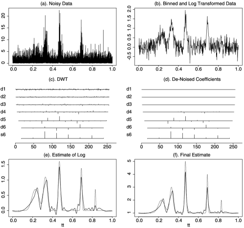
Figure 4: An example of nonparametric Gamma regression using the mean-matching VST and wavelet block thresholding.

We now turn to the NeighCoeff procedure. This procedure, introduced in Cai and Silverman (2001) for Gaussian regression, incorporates information about neighboring coefficients in a different way from the BlockJS procedure. NeighCoeff also thresholds the empirical coefficients in blocks, but estimates wavelet coefficients individually. It chooses a threshold for each coefficient by referencing not only to that coefficient but also to its neighbors. As shown in Cai and Silverman (2001), NeighCoeff outperforms BlockJS numerically, but with slightly inferior asymptotic properties.

Let the empirical coefficients $\{y_{j,k}\}$ be given same as before. To estimate a coefficient $\theta_{j,k}$ at resolution level $j$, we form a block of size $3$ by including the coefficient $y_{j,k}$ together with its immediate neighbors $y_{j,k-1}$ and $y_{j,k+1}$. (If periodic boundary conditions are not being used, then for the two coefficients at the boundary blocks, again of length $3$, are formed by only extending in one direction.) Estimate the coefficient $\theta_{j,k}$ by

$$\widehat{\theta}_{j,k}=\biggl{(}1-{\frac{2\log n}{nS_{j,k}^{2}}}\biggr{)}_{+}y_{j,k},$$ (26)

where $S_{j,k}^{2}=y_{j,k-1}^{2}+y_{j,k}^{2}+y_{j,k+1}^{2}$. The gross structure terms at the lowest resolution level are again estimated by $\widehat{\!\widetilde{\theta}}_{j_{0},k}=\widetilde{y}_{j_{0},k}$. The rest of the steps are same as before. Namely, the inverse DWT is applied to obtain an estimate $\widehat{G(f)}$ and the mean function $f$ is then estimated by $\widehat{f}_{\mathrm{NC}}(t)=G^{-1}(\widehat{G(f(t))})$.

We can envision a sliding window of size $3$ which moves one position each time and only the middle coefficient in the center is estimated for a given window. Each individual coefficient is thus shrunk by an amount that depends on the coefficient and on its immediate neighbors. Note that NeighCoeff uses a lower threshold level than the universal thresholding procedure of Donoho and Johnstone (1994). In NeighCoeff, a coefficient is estimated by zero only when the sum of squares of the empirical coefficient and its immediate neighbors is less than $2\sigma^{2}\log n$, or the average of the squares is less than ${\frac{2}{3}}\sigma^{2}\log n$.

4 Theoretical properties

In this section we investigate the asymptotic properties of the procedures proposed in Section 3. Numerical results will be given in Section 5.

We study the theoretical properties of our procedures over the Besov spaces that are by now standard for the analysis of wavelet regression methods. Besov spaces are a very rich class of function spaces and contain as special cases many traditional smoothness spaces such as Hölder and Sobolev spaces. Roughly speaking, the Besov space $B_{p,q}^{\alpha}$ contains functions having $\alpha$ bounded derivatives in $L^{p}$ norm, the third parameter $q$ gives a finer gradation of smoothness. Full details of Besov spaces are given, for example, in Triebel (1992) and DeVore and Popov (1988). A wavelet $\psi$ is called r-regular if $\psi$ has $r$ vanishing moments and $r$ continuous derivatives. For a given r-regular mother wavelet $\psi$ with $r>\alpha$ and a fixed primary resolution level $j_{0}$, the Besov sequence norm $\|\cdot\|_{b_{p,q}^{\alpha}}$ of the wavelet coefficients of a function $f$ is then defined by

$$\|f\|_{b_{p,q}^{\alpha}}=\|\underline{\xi}_{j_{0}}\|_{p}+\Biggl{(}\sum_{j=j_{0}}^{\infty}(2^{js}\|\underline{\theta}_{j}\|_{p})^{q}\Biggr{)}^{{1/q}},$$ (27)

where $\underline{\xi}_{j_{0}}$ is the vector of the father wavelet coefficients at the primary resolution level $j_{0}$, $\underline{\theta}_{j}$ is the vector of the wavelet coefficients at level $j$, and $s=\alpha+{\frac{1}{2}}-{\frac{1}{p}}>0$. Note that the Besov function norm of index $(\alpha,p,q)$ of a function $f$ is equivalent to the sequence norm (27) of the wavelet coefficients of the function. See Meyer (1992). We define

$$B_{p,q}^{\alpha}(M)=\{f;\|f\|_{b_{p,q}^{\alpha}}\leq M\}$$ (28)

and

$$F_{p,q}^{\alpha}(M,\varepsilon,v)=\{f\dvtx f\in B_{p,q}^{\alpha}(M),f(t)\in[\varepsilon,v]\mbox{ for all $t\in[0,1]$}\},$$ (29)

where $[\varepsilon,v]$ with $\epsilon<v$ is a compact set in the interior of the mean parameter space of the natural exponential family.

The following theorem shows that our estimators achieve near optimal global adaptation under integrated squared error for a wide range of Besov balls.

Theorem 2.

Suppose the wavelet $\psi$ is r-regular. Let $X_{i}\sim\operatorname{NQ}(f(t_{i})),i=1,\ldots,n,t_{i}={\frac{i}{n}}$. Let $T=cn^{{3/4}}$. Then the estimator $\widehat{f}_{\mathrm{BJS}}$ defined in (25) satisfies

$$\sup_{f\in F_{p,q}^{\alpha}(M,\varepsilon,v)}\mathbb{E}\|\widehat{f}_{\mathrm{BJS}}-f\|_{2}^{2}\leq\cases{Cn^{-{({2\alpha})/({1+2\alpha})}},\cr\qquad\mbox{$p\geq 2,\alpha\leq r$ and ${\dfrac{3}{2}\biggl{(}\alpha-{\dfrac{1}{p}}\biggr{)}>{\dfrac{2\alpha}{1+2\alpha}}}$},\vspace*{2pt}\cr Cn^{-{({2\alpha})/({1+2\alpha})}}(\log n)^{({2-p})/({p(1+2\alpha)})},\cr\qquad\mbox{$1\leq p<2,\alpha\leq r$ and ${\dfrac{3}{2}\biggl{(}\alpha-{\dfrac{1}{p}}\biggr{)}>{\dfrac{2\alpha}{1+2\alpha}}}$},}$$

and the estimator $\widehat{f}_{\mathrm{NC}}$ satisfies

$$\sup_{f\in F_{p,q}^{\alpha}(M,\varepsilon,v)}\mathbb{E}\|\widehat{f}_{\mathrm{NC}}-f\|_{2}^{2}\leq C\biggl{(}\frac{\log n}{n}\biggr{)}^{{({2\alpha})/({1+2\alpha})}},$$

$$\eqntext{p\geq 1,\alpha\leq r\mbox{ and }{\dfrac{3}{2}\biggl{(}\alpha-{\dfrac{1}{p}}\biggr{)}>{\dfrac{2\alpha}{1+2\alpha}}}.}$$ (30)

Remark 4.

Note that when $f(t)\in[\varepsilon,v]$, the condition $f\in B_{p,q}^{\alpha}(M)$ implies that there exists $M^{\prime}>0$ such that $G(f)\in B_{p,q}^{\alpha}(M^{\prime})$ with

$$M^{\prime}=c_{0}+cM\Biggl{[}\sum_{l=1}^{\lfloor\alpha\rfloor+1}c_{l}v^{l-1}+c_{\lfloor\alpha\rfloor+1}\Biggr{]}\qquad\mbox{for some }c>0,$$

where $c_{l}=\sup_{y\in[\varepsilon,v]}|G^{(l)}(y)|$ with $l=0,\ldots,\lfloor\alpha\rfloor+1$, since it follows from Theorem 3 on page 344 and Remark 3 on page 345 of Runst (1986) that

$$\|G(f)\|_{B_{p,q}^{\alpha}} \leq \|G(f)\|_{p}$$

$${}+c\|f\|_{B_{p,q}^{\alpha}}\Biggl{[}\sum_{l=1}^{\lfloor\alpha\rfloor+1}\bigl{\|}G^{(l)}(f)\bigr{\|}_{\infty}\|f\|_{\infty}^{l-1}+\bigl{\|}G^{\lfloor\alpha\rfloor+1}(f)\bigr{\|}_{\infty}\Biggr{]}.$$

Remark 5.

Simple algebra shows that $\frac{3}{2}(\alpha-{\frac{1}{p}})>{\frac{2\alpha}{1+2\alpha}}$ is equivalent to ${\frac{2\alpha^{2}-\alpha/3}{1+2\alpha}}>{\frac{1}{p}}$. This condition is needed to ensure that the discretization error over the Besov ball $B_{p,q}^{\alpha}(M)$ is negligible relative to the minimax risk. See Section 4.2 for more discussions.

For functions of spatial inhomogeneity, the local smoothness of the functions varies significantly from point to point and global risk given in Theorem 2 cannot wholly reflect the performance of estimators at a point. We use the local risk measure

$$R(\widehat{f}(t_{0}),f(t_{0}))=\mathbb{E}\bigl{(}\widehat{f}(t_{0})-f(t_{0})\bigr{)}^{2}$$ (31)

for spatial adaptivity.

The local smoothness of a function can be measured by its local Hölder smoothness index. For a fixed point $t_{0}\in(0,1)$ and $0<\alpha\leq 1$, define the local Hölder class $\Lambda^{\alpha}(M,t_{0},\delta)$ as follows:

$$\Lambda^{\alpha}(M,t_{0},\delta)=\{f\dvtx|f(t)-f(t_{0})|\leq M|t-t_{0}|^{\alpha},\mbox{for $t\in(t_{0}-\delta,t_{0}+\delta)$}\}.$$

If $\alpha>1$, then

$$\Lambda^{\alpha}(M,t_{0},\delta)=\bigl{\{}f\dvtx\bigl{|}f^{(\lfloor\alpha\rfloor)}(t)-f^{(\lfloor\alpha\rfloor)}(t_{0})\bigr{|}\leq M|t-t_{0}|^{\alpha^{\prime}}\mbox{ for $t\in(t_{0}-\delta,t_{0}+\delta)$}\bigr{\}},$$

where $\lfloor\alpha\rfloor$ is the largest integer less than $\alpha$ and $\alpha^{\prime}=\alpha-\lfloor\alpha\rfloor$. Define

$$F^{\alpha}(M,t_{0},\delta,\varepsilon,v)=\{f\dvtx f\in\Lambda^{\alpha}(M,t_{0},\delta),f(x)\in[\varepsilon,v]\mbox{ for all $x\in[0,1]$}\}.$$

In Gaussian nonparametric regression setting, it is a well-known fact that for estimation at a point, one must pay a price for adaptation. The optimal rate of convergence for estimating $f(t_{0})$ over function class $\Lambda^{\alpha}(M,t_{0},\delta)$ with $\alpha$ completely known is $n^{-2\alpha/(1+2\alpha)}$. Lepski (1990) and Brown and Low (1996) showed that one has to pay a price for adaptation of at least a logarithmic factor. It is shown that the local adaptive minimax rate over the Hölder class $\Lambda^{\alpha}(M,t_{0},\delta)$ is $(\log n/n)^{2\alpha/(1+2\alpha)}$.

The following theorem shows that our estimators achieve optimal local adaptation with the minimal cost.

Theorem 3.

Suppose the wavelet $\psi$ is r-regular with $1/6<\alpha\leq r$. Let $t_{0}\in(0,1)$ be fixed. Let $X_{i}\sim\operatorname{NQ}(f(t_{i})),i=1,\ldots,n,t_{i}=\frac{i}{n}$. Let $T=cn^{{3/4}}$. Then for $\widehat{f}=\widehat{f}_{\mathrm{BJS}}$ or $\widehat{f}_{\mathrm{NC}}$

$$\sup_{F^{\alpha}(M,t_{0},\delta,\varepsilon,v)}\mathbb{E}\bigl{(}\widehat{f}(t_{0})-f(t_{0})\bigr{)}^{2}\leq C\cdot\biggl{(}\frac{\log n}{n}\biggr{)}^{({2\alpha})/({1+2\alpha})}.$$ (32)

Theorem 3 shows that both estimators are spatially adaptive, without prior knowledge of the smoothness of the underlying functions.

4.1 Regression in general natural exponential families

We have so far focused on the nonparametric regression in the NEF–QVF families. Our method can be extended to the nonparametric regression in the general one-parameter natural exponential families where the variance is no longer a quadratic function of the mean.

Suppose we observe

$$Y_{i}\stackrel{{\scriptstyle\mathrm{ind}}}{{\sim}}\operatorname{NEF}(f(t_{i})),\qquad i=1,\ldots,n,t_{i}={\frac{i}{n}},$$ (33)

and wish to estimate the mean function $f(t)$. When the variance is not a quadratic function of the mean, the VST still exists, although the mean-matching VST does not. In this case, we set $a=b=0$ in (3) and define $H_{m}$ as

$$H_{m}(X)=G\biggl{(}{\frac{X}{m}}\biggr{)}.$$ (34)

We then apply the same four-step procedure, Binning–VST–Gaussian Regression–Inverse VST, as outlined in Section 3 where either BlockJS or NeighCoeff is used in the third step. Denote the resulting estimator by $\widehat{f}_{\mathrm{BJS}}$ and $\widehat{f}_{\mathrm{NC}}$, respectively.

The following theorem is an extension of Theorem 1 to the general one-parameter natural exponential families where the standard VST is used.

Theorem 4.

Let $f\in F^{d}(M,\varepsilon,v)$. Then $Y_{j}^{\ast}=G(\frac{Q_{j}}{m})$ can be written as

$$Y_{j}^{\ast}=G\biggl{(}f\biggl{(}{\frac{j}{T}}\biggr{)}\biggr{)}+\epsilon_{j}+m^{-{{1/2}}}Z_{j}+\xi_{j},\qquad j=1,2,\ldots,T,$$ (35)

where $Z_{j}\stackrel{{\scriptstyle\mathrm{i.i.d.}}}{{\sim}}N(0,1)$, $\epsilon_{j}$ are constants satisfying $|\epsilon_{j}|\leq{c}(m^{-1}+T^{-d})$ and consequently for some constant $C>0$

$${\frac{1}{T}}\sum_{j=1}^{T}\epsilon_{j}^{2}\leq C(m^{-2}+T^{-2d})$$ (36)

and $\xi_{j}$ are independent and “stochastically small” random variables satisfying that for any integer $k>0$ and any constant $a>0$

$$\mathbb{E}|\xi_{j}|^{k} \leq C_{k}\log^{2k}m\cdot(m^{-k}+T^{-dk})\quad\mbox{and}$$

$$\mathbb{P}(|\xi_{j}|>a) \leq C_{k}\log^{2k}m\cdot(m^{-k}+T^{-dk})a^{-k},$$

where $C_{k}>0$ is a constant depending only on $k,d$ and $M$.

The proof of Theorem 4 is similar to that of Theorem 1. Note that the bound for the deterministic error in (36) is different from the one given in equation (18). This difference affects the choice of the bin size.

Theorem 5.

Suppose the wavelet $\psi$ is r-regular. Let $X_{i}\sim\operatorname{NEF}(f(t_{i})),i=1,\ldots,n,t_{i}={\frac{i}{n}}$. Let $T=cn^{{1/2}}$. Then the estimator $\widehat{f}_{\mathrm{BJS}}$ satisfies

$$\sup_{f\in F_{p,q}^{\alpha}(M,\varepsilon,v)}\mathbb{E}\|\widehat{f}_{\mathrm{BJS}}-f\|_{2}^{2}\leq\cases{Cn^{-{({2\alpha})/({1+2\alpha})}},\cr\qquad\mbox{$p\geq 2,\alpha\leq r$ and $\biggl{(}\alpha-{\dfrac{1}{p}}\biggr{)}>{\dfrac{2\alpha}{1+2\alpha}}$},\vspace*{2pt}\cr Cn^{-{({2\alpha})/({1+2\alpha})}}(\log n)^{({2-p})/({p(1+2\alpha)})},\cr\qquad\mbox{$1\leq p<2,\alpha\leq r$ and $\biggl{(}\alpha-{\dfrac{1}{p}}\biggr{)}>{\dfrac{2\alpha}{1+2\alpha}}$},}$$

and the estimator $\widehat{f}_{\mathrm{NC}}$ satisfies

$$\sup_{f\in F_{p,q}^{\alpha}(M,\varepsilon,v)}\mathbb{E}\|\widehat{f}_{\mathrm{NC}}-f\|_{2}^{2}\leq C\biggl{(}\frac{\log n}{n}\biggr{)}^{{({2\alpha})/({1+2\alpha})}},$$

$$\eqntext{p\geq 1,\alpha\leq r\mbox{ and }{\biggl{(}\alpha-{\dfrac{1}{p}}\biggr{)}>{\dfrac{2\alpha}{1+2\alpha}}}.}$$ (38)

Remark 6.

Note that the number of bins here is $T=O(n^{{{1/2}}})$. This gives a larger bin size than that needed with NEF–QVF. Because the VST yields higher bias than the mean-matching VST in the case of NEF–QVF, it is necessary to use larger bins. The condition $(\alpha-{\frac{1}{p}})>{\frac{2\alpha}{1+2\alpha}}$ is also stronger than the condition $\frac{3}{2}(\alpha-{\frac{1}{p}})>{\frac{2\alpha}{1+2\alpha}}$ which is needed in the case of NEF–QVF. The functions are required to be smoother than before. This is due to the fact that both the approximation error and the discretization error are larger in this case. See Section 4.2 for more discussions.

We have the following result on spatial adaptivity.

Theorem 6.

Suppose the wavelet $\psi$ is r-regular with ${\frac{1}{2}}<\alpha\leq r$. Let $t_{0}\in(0,1)$ be fixed. Let $X_{i}\sim\operatorname{NEF}(f(t_{i})),i=1,\ldots,n,t_{i}=\frac{i}{n}$. Let $T=cn^{{{1/2}}}$. Then for $\widehat{f}=\widehat{f}_{\mathrm{BJS}}$ or $\widehat{f}_{\mathrm{NC}}$

$$\sup_{f\in F^{\alpha}(M,t_{0},\delta,\varepsilon,v)}\mathbb{E}\bigl{(}\widehat{f}(t_{0})-f(t_{0})\bigr{)}^{2}\leq C\biggl{(}\frac{\log n}{n}\biggr{)}^{({2\alpha})/({1+2\alpha})}.$$ (39)

Remark 7.

In Remark 1 we noted that some nonexponential families admit mean-matching variance stabilizing transformations. Although we do not pursue the issue in the current paper, we believe that analogs of our procedure can be developed for these families and the basic results in Theorems 2 and 3 can be extended to such situations. A different possibility is that the error distributions lie in a one parameter family that admits a VST that is not mean matching. In that case one could expect analogs of Theorems 5 and 6 to be valid.

4.2 Discussion

Our procedure begins with binning. This step makes the data more “normal” and at the same time reduces the number of observations from $n$ to $T$. This step in general does not affect the rate of convergence as long as the underlying function has certain minimum smoothness so that the bias induced by local averaging is negligible relative to the minimax estimation risk. While the number of observations is reduced by binning, the noise level is also reduced accordingly.

An important quantity in our method is the value of $T$, the number of bins, or equivalently the value of the bin size $m$. The choice of $T=cn^{3/4}$ for the NEF–QVF and $T=cn^{1/2}$ for the general NEF are determined by the bounds for the approximation error, the discretization error, and the stochastic error. For functions in the Besov ball $B^{\alpha}_{p,q}(M)$, the discretization error between the sampled function $\{G(f({j/T}))\dvtx j=1,\ldots,T\}$ and the whole function $G(f(t))$ can be bounded by $CT^{-2d}$ where $d=(\alpha-{\frac{1}{p}})\wedge 1$ (see Lemma 8 in Section 6.3). The approximation error ${\frac{1}{T}}\sum_{i=1}^{T}\epsilon_{i}^{2}$ can be bounded by $C(m^{-4}+T^{-2d})$ as in (18). In order to adaptively achieve the optimal rate of convergence, these deterministic errors need to be negligible relative to the minimax rate of convergence $n^{-{({2\alpha})/({1+2\alpha})}}$ for all $\alpha$ under consideration. That is, we need to have $m^{-4}=o(n^{-{({2\alpha})/({1+2\alpha})}})$ and $T^{-2d}=o(n^{-{({2\alpha})/({1+2\alpha})}})$. These conditions put constraints on both $m$ and $\alpha$ (and $p$). We choose $m=cn^{{1/4}}$ (or equivalently $T=cn^{{3/4}}$) to ensure that the approximation error is always negligible for all $\alpha$. This choice also guarantees that the stochastic error is under control. With this choice of $m$, we then need $\frac{3}{2}(\alpha-{\frac{1}{p}})>{\frac{2\alpha}{1+2\alpha}}$ or equivalently $\frac{2\alpha^{2}-\alpha/3}{1+2\alpha}>{\frac{1}{p}}$.

In the natural exponential family with a quadratic variance function, the existence of a mean-matching VST makes the approximation error small and this provides advantage over more general natural exponential families. For general NEF without a quadratic variance function, the approximation error ${\frac{1}{T}}\sum_{i=1}^{T}\epsilon_{i}^{2}$ is of order $m^{-2}+T^{-2d}$ instead of $m^{-4}+T^{-2d}$. Making it negligible for all $\alpha$ under consideration requires $m=cn^{{{1/2}}}$. With this choice of $m$, we require $\alpha-{\frac{1}{p}}>{\frac{2\alpha}{1+2\alpha}}$ or equivalently $\frac{2\alpha^{2}-\alpha}{1+2\alpha}>{\frac{1}{p}}$ in order to control the discretization error. In particular, this condition is satisfied if $\alpha\geq 1+{\frac{1}{p}}$.

In this paper we present a unified approach to nonparametric regression in the natural exponential families and the optimality results are given for Besov spaces. As mentioned in the Introduction, a wavelet shrinkage and modulation method was introduced in Antoniadis and Sapatinas (2001) for regression in the NEF–QVF and it was shown that the estimator attains the optimal rate over the classical Sobolev spaces with the smoothness index $\alpha>1/2$. In comparison to the results given in Antoniadis and Sapatinas (2001), our results are more general in terms of the function spaces as well as the natural exponential families. On the other hand, we require slightly stronger conditions on the smoothness of the underlying functions. It is intuitively clear that through binning and VST a certain amount of bias is introduced. The conditions $\frac{3}{2}(\alpha-{\frac{1}{p}})>{\frac{2\alpha}{1+2\alpha}}$ in the case of NEF–QVF and $\alpha-{\frac{1}{p}}>{\frac{2\alpha}{1+2\alpha}}$ in the general case are the minimum smoothness condition needed to ensure that the bias is under control. The bias in the general NEF case is larger and therefore the required smoothness condition is stronger.

5 Numerical study

In this section we study the numerical performance of our estimators. The procedures introduced in Section 3 are easily implementable. We shall first consider simulation results and then apply one of our procedures in the analysis of two real data sets.

5.1 Simulation results

As discussed the Section 2, there are several different versions of the VST in the literature and we have emphasized the importance of using the mean-matching VST for theoretical reasons. We shall now consider the effect of the choice of the VST on the numerical performance of the resulting estimator. To save space we only consider the Poisson and Bernoulli cases. We shall compare the numerical performance of the mean-matching VST with those of classical transformations by Bartlett (1936) and Anscombe (1948) using simulations. The transformation formulae are given as follows. (In the following tables and figures, we shall use MM for mean-matching.)

	MM	Bartlett	Anscombe
$\operatorname{Poi}(\lambda)$	$\sqrt{X+1/4}$	$\sqrt{X}$	$\sqrt{X+3/8}$
$\operatorname{Bin}(m,p)$	$\sin^{-1}\sqrt{\frac{X+1/4}{m+1/2}}$	$\sin^{-1}\sqrt{\frac{X}{m}}$	$\sin^{-1}\sqrt{\frac{X+3/8}{m+3/4}}$

Four standard test functions, Doppler, Bumps, Blocks and HeaviSine, representing different level of spatial variability are used for the comparison of the three VSTs. See Donoho and Johnstone (1994) for the formulae of the four test functions. These test functions are suitably normalized so that they are positive and taking values between 0 and 1 (in the binomial case). Sample sizes vary from a few hundred to a few hundred thousand. We use Daubechies’ compactly supported wavelet Symmlet 8 for wavelet transformation. As is the case in general, it is possible to obtain better estimates with different wavelets for different signals. But for uniformity, we use the same wavelet for all cases. Although our asymptotic theory only gives a justification for the choice of the bin size of order $n^{1/4}$ due to technical reasons, our extensive numerical studies have shown that the procedure works well when the number of counts in each bin is between 5 and 10 for the Poisson case, and similarly for the Bernoulli case the average number of successes and failures in each bin is between 5 and 10. We follow this guideline in our simulation study. Table 1 reports the average squared errors over 100 replications for the BlockJS thresholding. The sample sizes are $1280,5120,\ldots,327\mbox{,}680$ for the Bernoulli case and $640,2560,\ldots,163\mbox{,}840$ for the Poisson case. A graphical presentation is given in Figure 5.

Table 1: Mean squared error (MSE) from $100$ replications. The MSE is in units of $10^{-3}$ for Bernoulli case and $10^{-2}$ for Poisson case

	MM	Bartlett	Anscombe		MM	Bartlett	Anscombe
Bernoulli
Doppler				Bumps
00,1280	$12.117$	$11.197$	$12.673$	00,1280	$7.756$	$8.631$	$7.896$
00,5120	$3.767$	$3.593$	$4.110$	00,5120	$7.455$	$7.733$	$7.768$
20,480	$1.282$	$1.556$	$1.417$	020,480	$3.073$	$3.476$	$3.450$
81,920	$0.447$	$0.772$	$0.540$	081,920	$1.203$	$1.953$	$1.485$
327,680	$0.116$	$0.528$	$0.169$	327,680	$0.331$	$1.312$	$0.535$
Blocks				HeaviSine
00,1280	$18.451$	$17.171$	$18.875$	00,1280	$2.129$	$2.966$	$2.083$
00,5120	$7.582$	$6.911$	$7.996$	00,5120	$0.842$	$1.422$	$0.860$
20,480	$3.288$	$3.072$	$3.545$	020,480	$0.549$	$0.992$	$0.603$
81,920	$1.580$	$1.587$	$1.737$	081,920	$0.285$	$0.681$	$0.339$
327,680	$0.594$	$0.781$	$0.681$	327,680	$0.138$	$0.532$	$0.195$
Poisson
Doppler				Bumps
000,640	$8.101$	$8.282$	$8.205$	000,640	$107.860$	$103.696$	$109.023$
00,2560	$3.066$	$3.352$	$3.160$	00,2560	$70.034$	$68.616$	$70.495$
10,240	$1.069$	$1.426$	$1.146$	010,240	$24.427$	$24.268$	$24.653$
40,960	$0.415$	$0.743$	$0.502$	040,960	$9.427$	$9.469$	$9.620$
163,840	$0.108$	$0.461$	$0.190$	163840	$3.004$	$3.098$	$3.204$
Blocks				HeaviSine
000,640	$12.219$	$12.250$	$12.320$	000,640	$2.831$	$3.552$	$2.851$
00,2560	$5.687$	$6.209$	$5.724$	00,2560	$0.849$	$1.468$	$0.884$
10,240	$2.955$	$3.363$	$3.005$	010,240	$0.425$	$0.852$	$0.501$
40,960	$1.424$	$1.773$	$1.495$	040,960	$0.213$	$0.560$	$0.298$
163,840	$0.508$	$0.890$	$0.573$	163,840	$0.118$	$0.455$	$0.206$

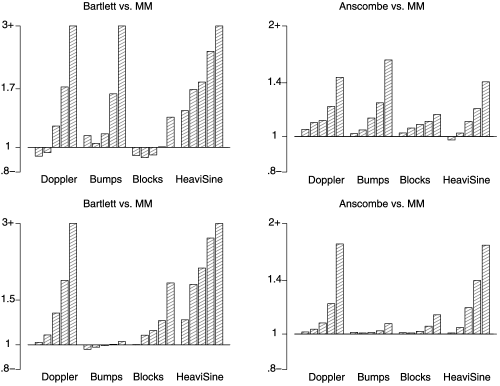
Figure 5: Left panels: the vertical bars represent the ratios of the MSE of the estimator using the Bartlett VST to the corresponding MSE of our estimator using the mean-matching VST. Right Panels: the bars represent the ratios of the MSE of the estimator using the Anscombe VST to the corresponding MSE of the estimator using the mean-matching VST. The higher the bar the better the relative performance of our estimator. The bars are plotted on a log scale and the original ratios are truncated at the value $3$ for the Bartlett VST and at $2$ for the Anscombe VST. For each signal the bars are ordered from left to right in the order of increasing sample size. The top row is for the Bernoulli case and the bottom row for the Poisson case.

Table 1 compares the performance of three nonparametric function estimators constructed from three VSTs and wavelet BlockJS thresholding for Bernoulli and Poisson regressions. The three VSTs are the mean-matching, Bartlett and Anscombe transformations given above. The results show the mean-matching VST outperforms the classical transformations for nonparametric estimation in most cases. The improvement becomes more significant as the sample size increases.

In the Poisson regression, the mean-matching VST outperforms the Bartlett VST in 17 out of 20 cases and uniformly outperforms the Anscombe VST in all 20 cases. The case of Bernoulli regression is similar: the mean-matching VST is better than the Bartlett VST in 15 out of 20 cases and better than the Anscombe VST in 19 out of 20 cases. Although the mean-matching VST does not uniformly dominate either the Bartlett VST or the Anscombe VST, the improvement of the mean-matching VST over the other two VSTs is significant as the sample size increases for all four test functions. The simulation results show that mean-matching VST yields good numerical results in comparison to other VSTs. These numerical findings is consistent with the theoretical results given in Section 4 which show that the estimator constructed from the mean-matching VST enjoys desirable adaptivity properties.

Table 2 reports the average squared errors over 100 replications for the NeighCoeff procedure in the same setting as those in Table 1. In comparison to BlockJS, the numerical performance of NeighCoeff is overall slightly better. Among the three VSTs, the mean-matching VST again outperforms both the Anscombe VST and Bartlett VST.

We have so far considered the effect of the choice of VST on the performance of the estimator. We now discuss the Poisson case in more detail and compare the numerical performance of our procedure with other estimators proposed in the literature. As mentioned in the Introduction, Besbeas, De Feis and Sapatinas (2004) carried out an extensive simulation studies comparing several nonparametric Poisson regression estimators including the estimator given in Donoho (1993). The estimator in Donoho (1993) was constructed by first applying the Anscombe (1948) VST to the binned data and by then using a wavelet procedure with a global threshold such as VisuShrink [Donoho and Johnstone (1994)] to the transformed data as if the data were actually Gaussian. Figure 6 plots the ratios of the MSE of Donoho’s estimator to the corresponding MSE of our estimator. The results show that our estimator outperforms Donoho’s estimator in all but one case and in many cases our estimator has the MSE less than one half and sometimes even one third of that of Donoho’s estimator.

Besbeas, De Feis and Sapatinas (2004) plotted simulation results of 27 procedures for six intensity functions (Smooth, Angles, Clipped Blocks, Bumps, Spikes and Bursts) with sample size 512 under the squared root of mean squared error (RMSE). We apply NeighCoeff and BlockJS procedures to data with exactly the same intensity functions. The following table reports the RMSE of NeighCoeff and BlockJS procedures based on 100 replications:

We compare our results with the plots of RMSE for 27 methods in Besbeas, De Feis and Sapatinas (2004). The NeighCoeff procedure dominates all 27 methods for signals Smooth and Spikes, outperforms most of procedures for signals Angles and Bursts, and performs slightly worse than average for signals Clipped Blocks and Bumps. The BlockJS procedure is comparable with the NeighCoeff procedure except for two signals Clipped Blocks and Bumps. We should note that an exact numerical comparison here is difficult as the results in Besbeas, de Feis and Sapatinas (2004) were given in plots, not numerical values.

Table 2: Mean squared error (MSE) from $100$ replications for the NeighCoeff thresholding. The MSE is in units of $10^{-3}$ for Bernoulli case and $10^{-2}$ for Poisson case

	MM	Bartlett	Anscombe		MM	Bartlett	Anscombe
Bernoulli
Doppler				Bumps
00,1280	$8.574$	$8.569$	$8.959$	00,1280	$7.085$	$7.741$	$7.361$
00,5120	$2.935$	$3.211$	$3.129$	00,5120	$6.810$	$7.052$	$7.180$
20,480	$1.029$	$1.380$	$1.143$	020,480	$2.846$	$3.364$	$3.204$
81,920	$0.377$	$0.800$	$0.438$	081,920	$0.958$	$1.789$	$1.220$
327,680	$0.138$	$0.556$	$0.186$	327,680	$0.264$	$1.274$	$0.458$
Blocks				HeaviSine
00,1280	$14.838$	$13.964$	$15.336$	00,1280	$2.072$	$3.092$	$2.010$
00,5120	$7.129$	$6.615$	$7.511$	00,5120	$0.822$	$1.479$	$0.841$
20,480	$3.131$	$2.904$	$3.388$	020,480	$0.529$	$1.007$	$0.580$
81,920	$1.266$	$1.350$	$1.400$	081,920	$0.235$	$0.660$	$0.286$
327,680	$0.469$	$0.680$	$0.553$	327,680	$0.102$	$0.512$	$0.156$
Poisson
Doppler				Bumps
000,640	$7.789$	$8.030$	$7.888$	000,640	$105.624$	$101.486$	$106.76$
00,2560	$3.112$	$3.398$	$3.200$	00,2560	$69.627$	$68.175$	$70.105$
10,240	$1.006$	$1.362$	$1.081$	010,240	$24.448$	$24.304$	$24.672$
40,960	$0.402$	$0.731$	$0.488$	040,960	$9.312$	$9.341$	$9.507$
163,840	$0.106$	$0.460$	$0.187$	163,840	$3.005$	$3.102$	$3.203$
Blocks				HeaviSine
000,640	$12.301$	$12.141$	$12.412$	000,640	$2.679$	$3.465$	$2.672$
00,2560	$5.719$	$6.229$	$5.758$	00,2560	$0.903$	$1.427$	$0.977$
10,240	$2.985$	$3.363$	$3.046$	010,240	$0.429$	$0.852$	$0.505$
40,960	$1.399$	$1.755$	$1.469$	040,960	$0.215$	$0.562$	$0.300$
163,840	$0.504$	$0.877$	$0.572$	163,840	$0.120$	$0.453$	$0.209$

	Smooth	Angles	Clipped blocks	Bumps	Spikes	Bursts
NeighCoeff	1.773	2.249	5.651	4.653	2.096	2.591
BlockJS	1.760	2.240	6.492	5.454	2.315	2.853

5.2 Real data applications

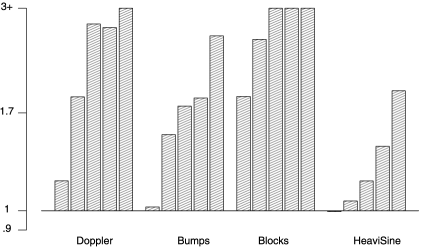
Figure 6: The vertical bars represent the ratios of the MSE of Donoho’s estimator to the corresponding MSE of our estimator. The higher the bar the better the relative performance of our estimator. The bars are plotted on a log scale and the original ratios are truncated at the value $3$. For each signal the bars are ordered from left to right in the order of increasing sample size.

We now demonstrate our estimation method in the analysis of two real data sets, a gamma-ray burst data set (GRBs) and a packet loss data set. These two data sets have been discussed in Kolaczyk and Nowak (2005).

Figure 7: Gamma-ray burst. Histogram of BATSE $551$ with $1024$ bins (top panel). Estimator based on $1024$ bin (middle panel). Estimator with $512$ bins (bottom panel).

Cosmic gamma-ray bursts were first discovered in the late 1960s. In 1991, NASA launched the Compton Gamma Ray Observatory and its Burst and Transient Source Explorer (BATSE) instrument, a sensitive gamma-ray detector. Much burst data has been collected since then, followed by extensive studies and many important scientific discoveries during the past few decades; however, the source of GRBs remains unknown [Kaneko (2005)]. For more details see the NASA website http://www.batse.msfc.nasa.gov/batse/. GRBs seem to be connected to massive stars and become powerful probes of the star formation history of the universe. However not many redshifts are known and there is still much work to be done to determine the mechanisms that produce these enigmatic events. Statistical methods for temporal studies are necessary to characterize their properties and hence to identify the physical properties of the emission mechanism. One of the difficulties in analyzing the time profiles of GRBs is the transient nature of GRBs which means that the usual assumptions for Fourier transform techniques do not hold [Quilligan et al. (2002)]. We may model the time series data by an inhomogeneous Poisson process, and apply our wavelet procedure. The data set we use is called BATSE 551 with the sample size 7808. In Figure 7, the top panel is the histogram of the data with 1024 bins such that the number of observations in each bin would be between 5 and 10. In fact we have on average 7.6 observations. The middle panel is the estimate of the intensity function using our procedure. If we double the width of each bin, that is, the total number of bins is now 512, the new estimator in the bottom panel is noticeably different from previous one since it does not capture the fine structure from time 200 to 300. The study of the number of pulses in GRBs and their time structure is important to provide evidence for rotation powered systems with intense magnetic fields and the added complexity of a jet.

Figure 8: Packet loss data. Histogram with $2048$ bins (top panel). Estimator based on the binned data (bottom panel).

Packet loss describes an error condition in internet traffic in which data packets appear to be transmitted correctly at one end of a connection, but never arrive at the other. So, if 10 packets were sent out, but only 8 made it through, then there would be 20% overall packet loss. The following data were originally collected and analyzed by Yajnik et al. (1999). The objective is to understand packet loss by modeling. It measures the reliability of a connection and is of fundamental importance in network applications such as audio/video conferencing and Internet telephony. Understanding the loss seen by such applications is important in their design and performance analysis. The measurements are of loss as seen by packet probes sent at regular time intervals. The packets were transmitted from the University of Massachusetts at Amherst to the Swedish Institute of Computer Science. The records note whether each packet arrived or was lost. It is a Bernoulli time series, and can be naturally modeled as Binomial after binning the data. Figure 8 gives the histogram and our corresponding estimator. The average sum of failures in each bin is about 10. The estimator in Kolaczyk and Nowak (2005) is comparable to ours. But our procedure is more easily implemented.

6 Proofs

In this section we give proofs for Theorems 1, 2 and 5. Theorems 3 and 6 can be proved in a similar way as Theorem 4 in Brown, Cai and Zhou (2008) by applying Proposition 1 in Section 6.3. We begin by proving Lemmas 1 and 3 as well as an additional technical result, Lemma 4. These results are needed to establish Theorem 1 in which an approximation bound between our model and a Gaussian regression model is given explicitly. Finally we apply Theorem 1 and risk bounds for block thresholding estimators in Proposition 1 to prove Theorems 2 and 5.

6.1 Proof of preparatory technical results

Proof of Lemma 1 We only prove (4), the first part of the lemma. The proof for equation (5), the second part, is similar and simpler. By Taylor’s expansion we write

$$G\biggl{(}\frac{X+a}{m+b}\biggr{)}-G(\mu(\eta))=T_{1}+T_{2}+T_{3}+T_{4},$$

where

$$T_{1} = G^{\prime}(\mu(\eta))\biggl{(}\frac{X+a}{m+b}-\mu(\eta)\biggr{)},\qquad T_{2}=\frac{1}{2}G^{\prime\prime}(\mu(\eta))\biggl{(}\frac{X+a}{m+b}-\mu(\eta)\biggr{)}^{2},$$

$$T_{3} = \frac{1}{6}G^{\prime\prime\prime}(\mu(\eta))\biggl{(}\frac{X+a}{m+b}-\mu(\eta)\biggr{)}^{3},\qquad T_{4}=\frac{1}{24}G^{(4)}(\mu^{\ast})\biggl{(}\frac{X+a}{m+b}-\mu(\eta)\biggr{)}^{4}$$

and $\mu^{\ast}$ is in between $\frac{X+a}{m+b}$ and $\mu(\eta)$. By definition, $G^{\prime}(\mu(\eta))=I(\eta)^{-1/2}$ with $I(\eta)=\mu^{\prime}(\eta)$ which is also $V(\mu(\eta))$ in (2), then

$$G^{\prime\prime}(\mu(\eta))\mu^{\prime}(\eta)=-\tfrac{1}{2}I(\eta)^{-3/2}I^{\prime}(\eta),$$

that is,

$$G^{\prime\prime}(\mu(\eta))=-\tfrac{1}{2}I(\eta)^{-5/2}I^{\prime}(\eta),$$

then

$$\mathbb{E}T_{1} = I(\eta)^{-1/2}\frac{a-\mu(\eta)b}{m+b},$$

$$\mathbb{E}T_{2} = -\frac{1}{4}I(\eta)^{-5/2}I^{\prime}(\eta)\biggl{[}\biggl{(}\frac{a-\mu(\eta)b}{m+b}\biggr{)}^{2}+\frac{mI(\eta)}{(m+b)^{2}}\biggr{]}.$$

Note that $G^{\prime\prime}(\mu(\eta))$ is uniformly bounded on $\Theta$ by the assumption in the lemma, then we have

$$\mathbb{E}(T_{1}+T_{2}) = \frac{m}{(m+b)^{2}I(\eta)^{1/2}}\biggl{(}a-\mu(\eta)b-\frac{\mu^{\prime\prime}(\eta)}{4\mu^{\prime}(\eta)}\biggr{)}+O\biggl{(}\frac{1}{m^{2}}\biggr{)}$$

$$= \frac{1}{mI(\eta)^{1/2}}\biggl{(}a-\mu(\eta)b-\frac{\mu^{\prime\prime}(\eta)}{4\mu^{\prime}(\eta)}\biggr{)}+O\biggl{(}\frac{1}{m^{2}}\biggr{)}.$$

It is easy to show that

$$|\mathbb{E}T_{3}|=\biggl{|}\frac{1}{6}G^{\prime\prime\prime}(\mu(\eta))\mathbb{E}\biggl{(}\frac{X+a}{m+b}-\mu(\eta)\biggr{)}^{3}\biggr{|}=O\biggl{(}\frac{1}{m^{2}}\biggr{)},$$ (41)

since $|\mathbb{E}(X/m-\mu(\eta))^{3}|=O(\frac{1}{m^{2}})$. For any $\epsilon>0$ it is known that

$$\mathbb{P}\biggl{\{}\biggl{|}\frac{X+a}{m+b}-\mu(\eta)\biggr{|}>\epsilon\biggr{\}}\leq\mathbb{P}\{|X/m-\mu(\eta)|>\epsilon/2\},$$

which decays exponentially fast as $m\rightarrow\infty$ [see, e.g., Petrov (1975)]. This implies $\mu^{\ast}$ is in the interior of the natural parameter space and then $G^{(4)}(\mu^{\ast})$ is bounded with probability approaching to $1$ exponentially fast. Thus we have

$$|\mathbb{E}T_{4}|\leq C\mathbb{E}\biggl{(}\frac{X+a}{m+b}-\mu(\eta)\biggr{)}^{4}=O\biggl{(}\frac{1}{m^{2}}\biggr{)}.$$ (42)

Equation (4) then follows immediately by combining equations (6.1)–(42). Proof of Lemma 2 The proof is similar to Corollary 1 of Zhou (2006). Let $\widetilde{X}=\frac{X-m\mu}{\sqrt{mV}}$. It is shown in Komlós, Major and Tusnády (1975) that there exists a standard normal random variable $Z\sim N(0,1)$ and constants $\varepsilon,c_{4}>0$ not depending on $m$ such that whenever the event $A=\{|\widetilde{X}|\leq\varepsilon\sqrt{m}\}$ occurs,

$$|\widetilde{X}-Z|<\frac{c_{4}}{\sqrt{m}}+\frac{c_{4}}{\sqrt{m}}\widetilde{X}^{2}.$$ (43)

Obviously inequality (43) still holds when $|\widetilde{X}|\leq\varepsilon_{1}\sqrt{m}$ for $0<\varepsilon_{1}\leq\varepsilon$. Let’s choose $\varepsilon_{1}$ small enough such that $c_{4}\varepsilon_{1}^{2}<1/2$. When $|\widetilde{X}|\leq\varepsilon_{1}\sqrt{m}$, we have $|\widetilde{X}-Z|\leq\frac{c_{4}}{\sqrt{m}}+\frac{1}{2}|\widetilde{X}|$ from (43), which implies $|\widetilde{X}|-|Z|\leq\frac{c_{4}}{\sqrt{m}}+\frac{1}{2}|\widetilde{X}|$ by the triangle inequality, that is, $|\widetilde{X}|\leq\frac{2c_{4}}{\sqrt{m}}+2|Z|$, so we have

$$|\widetilde{X}-Z|\leq\frac{c_{4}}{\sqrt{m}}+\frac{c_{4}}{\sqrt{m}}\biggl{(}\frac{2c_{4}}{\sqrt{m}}+2|Z|\biggr{)}^{2}\leq c_{2}Z^{2}+c_{3}$$

for some constants $c_{1},c_{2}>0$. Proof of Lemma 3 By Taylor’s expansion we write

$$G\biggl{(}\frac{X+a}{m+b}\biggr{)}-G(\mu)=G^{\prime}(\mu)\biggl{(}\frac{X+a}{m+b}-\mu\biggr{)}+\frac{1}{2}G^{\prime\prime}(\mu^{\ast})\biggl{(}\frac{X+a}{m+b}-\mu\biggr{)}^{2}.$$

Recall that $|\epsilon|=|\mathbb{E}G(\frac{X+a}{m+b})-G({\mu})|=O(m^{-2})$ from Lemma 1, and $Z$ is a standard normal variable satisfying (13), and

$$\xi=G\biggl{(}{\frac{X+a}{m+b}}\biggr{)}-G({\mu})-\epsilon-m^{-{{1/2}}}Z.$$ (44)

We write $\xi=\xi_{1}+\xi_{2}+\xi_{3}$, where

$$\xi_{1} = G^{\prime}(\mu)\biggl{(}\frac{X+a}{m+b}-\frac{X}{m}\biggr{)}-\epsilon=G^{\prime}(\mu)\frac{am-bX}{m(m+b)}-\epsilon,$$

$$\xi_{2} = G^{\prime}(\mu)\Biggl{(}\frac{X}{m}-\mu-\sqrt{\frac{V}{m}}Z\Biggr{)}=\frac{G^{\prime}(\mu)}{m}\bigl{(}X-m\mu-\sqrt{mV}Z\bigr{)},$$

$$\xi_{3} = \frac{1}{2}G^{\prime\prime}(\mu^{\ast})\biggl{(}\frac{X+a}{m+b}-\mu\biggr{)}^{2}=\frac{1}{2}G^{\prime\prime}(\mu^{\ast})\biggl{(}\frac{X-m\mu}{m+b}+\frac{a-b\mu}{m+b}\biggr{)}^{2}.$$

It is easy to see that $\mathbb{E}|\xi_{1}|^{k}\leq C_{k}m^{-k}$. Since $\mathbb{P}\{|X-m\mu|\geq c_{1}m\}$ is exponentially small [cf. Komlós, Major and Tusnády (1975)], an application of Lemma 2 implies $\mathbb{E}|\xi_{2}|^{k}\leq C_{k}m^{-k}$. Note that on the event $\{|X-m\mu|\leq c_{1}m\}$, $G^{\prime\prime}(\mu^{\ast})$ is bounded for $m$ sufficiently large, then $\mathbb{E}|\xi_{3}|^{k}\leq C_{k}m^{-k}$ by observing that $\mathbb{E}[(X-m\mu)/\sqrt{m}]^{2k}\leq C_{k}^{\prime}$. The inequality $\mathbb{E}|\xi|^{k}\leq C_{k}m^{-k}$ then follows immediately by combining the moments bounds for $\xi_{1}$, $\xi_{2}$ and $\xi_{3}$. The second bound in (16) is a direct consequence of the first one and Markov inequality.

The variance stabilizing transformation considered in Section 2 is for i.i.d. observations. In the function estimation procedure, observations in each bin are independent but not identically distributed. However, observations in each bin can be treated as i.i.d. random variables through coupling. Let $X_{i}\sim\operatorname{NQ}(\mu_{i})$, $i=1,\ldots,m$, be independent. Here the means $\mu_{i}$ are “close” but not equal. Let $X_{i,c}$ be a set of i.i.d. random variables with $X_{i,c}$ $\sim\operatorname{NQ}(\mu_{c})$. We define

$$D=G\biggl{(}\frac{\sum_{i=1}^{m}X_{i}+a}{m+b}\biggr{)}-G\biggl{(}\frac{\sum_{i=1}^{m}X_{i,c}+a}{m+b}\biggr{)}.$$

If $\mu_{c}=\max_{i}\mu_{i}$, it is easy to see $\mathbb{E}D\leq 0$ since $X_{i,c}$ is stochastically larger than $X_{i}$ for all $i$ [see, e.g., Lehmann and Romano (2005)]. Similarly, $\mathbb{E}D\geq 0$ when $\mu_{c}=\min_{i}\mu_{i}$. We will select a

$$\mu_{c}^{\ast}\in\Bigl{[}\min_{i}\mu_{i},\max_{i}\mu_{i}\Bigr{]}$$ (45)

such that $\mathbb{E}D=0$, which is possible by the intermediate value theorem. In the following lemma we construct i.i.d. random variables $X_{i,c}$ $\sim\operatorname{NQ}(\mu_{c}^{\ast})$ on the sample space of $X_{i}$ such that $D$ is very small and has negligible contribution to the final risk bounds in Theorems 2 and 3.

Lemma 4

Let $X_{i}\sim\operatorname{NQ}(\mu_{i})$, $i=1,\ldots,m$, be independent with $\mu_{i}\in[\varepsilon,v]$, a compact subset in the interior of the mean parameter space of the natural exponential family. Assume that $|{\min_{i}\mu_{i}-\max_{i}\mu_{i}}|\leq C\delta$. Then there are i.i.d. random variables $X_{i,c}$ where $X_{i,c}\sim\operatorname{NQ}(\mu_{c}^{\ast})$ with $\mu_{c}^{\ast}\in[\min_{i}\mu_{i},\max_{i}\mu_{i}]$ such that $\mathbb{E}D=0$ and:

$$\mathbb{P}(\{X_{i}\neq X_{i,c}\})\leq C\delta;$$ (46)

and for any fixed integer $k\geq 1$ there exists a constant $C_{k}>0$ such that for all $a>0$,

$$\mathbb{E}|D|^{k} \leq C_{k}\log^{2k}m\cdot(m^{-k}+\delta^{-k})\quad\mbox{and}$$

$$\mathbb{P}(|D|>a) \leq C_{k}\frac{\log^{2k}m}{a^{k}}(m^{-k}+\delta^{-k}).$$

(i) There is a classical coupling identity for the Total variation distance. Let $P$ and $Q$ be distributions of two random variables $X$ and $Y$ on the same sample space, respectively, then there is a random variable $Y_{c}$ with distribution $Q$ such that $\mathbb{P}(X\neq Y_{c})=|P-Q|_{\mathrm{TV}}$. See, for example, page 256 in Pollard (2002). The proof of inequality (46) follows from that identity and the inequality that $|{\operatorname{NQ}(\mu_{i})-\operatorname{NQ}(\mu_{c}^{\ast})}|_{\mathrm{TV}}\leq C|\mu_{i}-\mu_{c}^{\ast}|$ for some $C>0$ which only depends on the family of the distribution of $X_{i}$ and $[\varepsilon,v]$.

(ii) Using Taylor’s expansion we can rewrite $D$ as $D=G^{\prime}(\zeta)\frac{\sum_{i=1}^{m}(X_{i}-X_{i,c})}{m+b}$ for some $\zeta$ in between $\frac{\sum_{i=1}^{m}X_{i}+a}{m+b}$ and $\frac{\sum_{i=1}^{m}X_{i,c}+a}{m+b}$. Since the distribution $X_{i}$ is in exponential family, then $\mathbb{P}(\max_{i}|X_{i}-X_{i,c}|>\log^{2}m)\leq C_{k^{\prime}}m^{-k^{\prime}}$ for all $k^{\prime}>0$, which implies $\mathbb{E}|X_{i}-X_{i,c}|^{k}\leq C_{k}\delta\log^{2k}m$ fo all positive integer $k$. Since $X_{i}-X_{i,c}$ are independent, it can be shown that

$$\mathbb{E}\Biggl{(}\frac{1}{m}\sum_{i=1}^{m}|X_{i}-X_{i,c}|\Biggr{)}^{k}$$

$$\qquad\leq\frac{1}{m^{k}}\sum_{k_{1}+\cdots+k_{m}=k}{\pmatrix{k\cr k_{1},\ldots,k_{m}}}E|X_{1}-X_{1,c}|_{1}^{k_{1}}\cdots E|X_{m}-X_{m,c}|_{m}^{k_{m}}$$

$$\qquad=\frac{1}{m^{k}}\sum_{j=1}^{k}\mathop{\sum_{k_{1}+\cdots+k_{m}=k,}}_{\operatorname{Card}\{i,k_{i}\geq 1\}=j}{\pmatrix{k\cr k_{1},\ldots,k_{m}}}E|X_{1}-X_{1,c}|_{1}^{k_{1}}\cdots E|X_{m}-X_{m,c}|_{m}^{k_{m}}$$

$$\qquad\leq C_{k}\frac{\log^{2k}m}{m^{k}}\sum_{j=1}^{k}\delta^{j}\cdot\operatorname{Card}\bigl{\{}(k_{1},\ldots,k_{m})\dvtx k_{1}+\cdots+k_{m}=k,$$

$$\hskip 200.4pt\operatorname{Card}\{i,k_{i}\geq 1\}=j\bigr{\}}$$

$$\qquad\leq C_{k}^{\prime}\frac{\log^{2k}m}{m^{k}}\Biggl{(}\sum_{j=1}^{k}m^{j}\delta^{j}\Biggr{)}=C_{k}^{\prime}\log^{2k}m\Biggl{(}\sum_{j=1}^{k}m^{j-k}\delta^{j}\Biggr{)},$$

where the last inequality follows from the facts that $k$ is fixed and finite and

$$\operatorname{Card}\bigl{\{}(k_{1},\ldots,k_{m})\dvtx k_{1}+\cdots+k_{m}=k,\operatorname{Card}\{i,k_{i}\geq 1\}=j\bigr{\}}$$

$$\qquad={\pmatrix{m\cr j}}\operatorname{Card}\{(k_{1},\ldots,k_{j})\dvtx k_{1}+\cdots+k_{j}=k,k_{i}\geq 1\}$$

$$\qquad\leq{\pmatrix{m\cr j}}k^{k}\leq{m}^{j}k^{k}.$$

Note that $\frac{m^{-k}+\delta^{k}}{m^{j-k}\delta^{j}}=\frac{1}{(m\delta)^{j}}+(m\delta)^{k-j}\geq 1$ for all $k\geq j\geq 1$, then

$$\mathbb{E}\Biggl{(}\frac{1}{m}\sum_{i=1}^{m}|X_{i}-X_{i,c}|\Biggr{)}^{k}\leq C_{k}^{\prime\prime}\log^{2k}m\cdot(m^{-k}+\delta^{k}).$$

Thus the first inequality in (4) follows immediately by observing that $G^{\prime}(\zeta)$ is bounded with a probability approaching to $1$ exponentially fast. The second bound is an immediate consequence of the first one and Markov inequality.

Remark 8.

The unknown function $f$ in a Besov ball $B_{p,q}^{\alpha}(M)$ has Hölder smoothness $d=\min(\alpha-{\frac{1}{p}},1)$, then $\delta$ in Lemma 4 can be chosen to be $T^{-d}$. The standard deviation of normal noise in equation (17) is $1/\sqrt{m}$. From the assumptions in Theorems 2 or 3 we see $m^{1/2}T^{-d}\log^{2}m$ converges to $0$ as a power of $n$, then

$$\mathbb{P}\bigl{(}|D|>1/\sqrt{m}\bigr{)}$$

$$\qquad\leq C_{k}\bigl{[}(m^{-1/2}\log^{2}m)m^{-k}+\bigl{(}\sqrt{m}T^{-d}\log^{2}m\bigr{)}^{k}\bigr{]}\qquad\mbox{for all }k\geq 1,$$

which converges to $0$ faster than any polynomial of $m$. This implies the contribution of $D$ to the final risk bounds in all major theorems is negligible as shown in later sections.

6.2 Proof of Theorem 1

From Lemma 4, there exist $Y_{j,c}^{\ast}$ where $X_{i,c}\sim\operatorname{NQ}(f_{j}^{\ast})$ with

$$f_{j,c}^{\ast}\in\biggl{[}\min_{jm+1\leq i\leq(j+1)m}f\biggl{(}\frac{i}{n}\biggr{)},\max_{jm+1\leq i\leq(j+1)m}f\biggl{(}\frac{i}{n}\biggr{)}\biggr{]}$$

as in (45) such that

$$\mathbb{E}[Y_{j}^{\ast}-Y_{j,c}^{\ast}] = 0,$$ (48)

$$\mathbb{E}|Y_{j}^{\ast}-Y_{j,c}^{\ast}|^{k} \leq C_{k}\log^{2k}m\cdot(m^{-k}+T^{-dk}),$$ (49)

$$\mathbb{P}(|Y_{j}^{\ast}-Y_{j,c}^{\ast}|>a) \leq C_{k}\frac{\log^{2k}m}{a^{k}}(m^{-k}+T^{-dk}).$$ (50)

Lemmas 1, 2 and 3 together yield

$$Y_{j,c}^{\ast}=G(f_{j,c}^{\ast})+\epsilon_{j}+m^{-{{1/2}}}Z_{j}+\xi_{j},\qquad j=1,2,\ldots,T,$$ (51)

and

$$\qquad|\epsilon_{j}|\leq Cm^{-2},\qquad\mathbb{E}|\xi_{j}|^{k}\leq C_{k}m^{-k}\quad\mbox{and}\quad\mathbb{P}(|\xi_{j}|>a)\leq C_{k}(am)^{-k}.$$ (52)

Note that

$$\biggl{|}G(f_{j,c}^{\ast})-G\biggl{(}f\biggl{(}\frac{j}{T}\biggr{)}\biggr{)}\biggr{|}\leq CT^{-d}.$$ (53)

Theorem 1 then follows immediately by combining equations (48)–(53).

6.3 Risk bound for wavelet thresholding

We collect here a few technical results that are useful for the proof of the main theorems. We begin with the following moment bounds for an orthogonal transform of independent variables. See Brown et al. (2010) for a proof.

Lemma 5

Let $X_{1},\ldots,X_{n}$ be independent variables with $\mathbb{E}(X_{i})=0$ for $i=1,\ldots,n$. Suppose that $\mathbb{E}|X_{i}|^{k}<M_{k}$ for all $i$ and all $k>0$ with $M_{k}>0$ some constant not depending on $n$. Let $Y=WX$ be an orthogonal transform of $X=(X_{1},\ldots,X_{n})^{\prime}$. Then there exist constants $M_{k}^{\prime}$ not depending on $n$ such that $\mathbb{E}|Y_{i}|^{k}<M_{k}^{\prime}$ for all $i=1,\ldots,n$ and all $k>0$.

Lemma 6 below provides an oracle inequality for block thresholding estimators without the normality assumption.

Lemma 6

Suppose $y_{i}=\theta_{i}+z_{i},i=1,\ldots,L$, where $\theta_{i}$ are constants and $z_{i}$ are random variables. Let $S^{2}=\sum_{i=1}^{L}y_{i}^{2}$ and let $\widehat{\theta}_{i}=(1-{\frac{\lambda L}{S^{2}}})_{+}y_{i}$. Then

$$\mathbb{E}\|\widehat{\theta}-\theta\|_{2}^{2}\leq\|\theta\|_{2}^{2}\wedge 4\lambda L+4\mathbb{E}[\|z\|_{2}^{2}I(\|z\|_{2}^{2}>\lambda L)].$$ (54)

It is easy to verify that $\|\widehat{\theta}-y\|_{2}^{2}\leq\lambda L$. Hence

$$\mathbb{E}[\|\widehat{\theta}-\theta\|_{2}^{2}I(\|z\|_{2}^{2}>\lambda L)]$$

$$\qquad\leq 2\mathbb{E}[\|\widehat{\theta}-y\|_{2}^{2}I(\|z\|_{2}^{2}>\lambda L)]+2\mathbb{E}[\|y-\theta\|_{2}^{2}I(\|z\|_{2}^{2}>\lambda L)]$$

(55)

$$\qquad\leq 2\lambda L\mathbb{P}(\|z\|_{2}^{2}>\lambda L)+2\mathbb{E}[\|z\|_{2}^{2}I(\|z\|_{2}^{2}>\lambda L)]$$

$$\qquad\leq 4\mathbb{E}[\|z\|_{2}^{2}I(\|z\|_{2}^{2}>\lambda L)].$$

On the other hand,

$$\mathbb{E}[\|\widehat{\theta}-\theta\|_{2}^{2}I(\|z\|_{2}^{2}\leq\lambda L)]$$

(56)

$$\qquad\leq\mathbb{E}[(2\|\widehat{\theta}-y\|_{2}^{2}+2\|y-\theta\|_{2}^{2})I(\|z\|_{2}^{2}\leq\lambda L)]\leq 4\lambda L.$$

Note that when $S^{2}\leq\lambda L$, $\widehat{\theta}=0$ and hence $\|\widehat{\theta}-\theta\|_{2}^{2}=\|\theta\|_{2}^{2}$. When $\|z\|_{2}^{2}\leq\lambda L$ and $S^{2}>\lambda L$,

$$\|\widehat{\theta}-\theta\|_{2}^{2} = \sum_{i}\biggl{[}\biggl{(}1-{\frac{\lambda L}{S^{2}}}\biggr{)}y_{i}-\theta_{i}\biggr{]}^{2}=\biggl{(}1-{\frac{\lambda L}{S^{2}}}\biggr{)}\biggl{[}S^{2}-\lambda L-2\sum_{i}\theta_{i}y_{i}\biggr{]}+\|\theta\|_{2}^{2}$$

$$= \biggl{(}1-{\frac{\lambda L}{S^{2}}}\biggr{)}\biggl{[}\sum(\theta_{i}+z_{i})^{2}-\lambda L-2\sum_{i}\theta_{i}(\theta_{i}+z_{i})\biggr{]}+\|\theta\|_{2}^{2}$$

$$= \biggl{(}1-{\frac{\lambda L}{S^{2}}}\biggr{)}(\|z\|_{2}^{2}-\lambda L-\|\theta\|_{2}^{2})+\|\theta\|_{2}^{2}\leq\|\theta\|_{2}^{2}.$$

Hence $\mathbb{E}[\|\widehat{\theta}-\theta\|_{2}^{2}I(\|z\|_{2}^{2}\leq\lambda L)]\leq\|\theta\|_{2}^{2}$ and ( 54) follows by combining this with (6.3) and (6.3).

The following bounds concerning a central chi-square distribution are from Cai (2002).

Lemma 7

Let $X\sim\chi_{L}^{2}$ and $\lambda>1$. Then

$$\mathbb{P}(X\geq\lambda L) \leq e^{-{{L/2}}(\lambda-\log\lambda-1)}\quad\mbox{and}$$

$$\mathbb{E}XI(X\geq\lambda L) \leq \lambda Le^{-{{L/2}}(\lambda-\log\lambda-1)}.$$

From (17) in Theorem 1 we can write ${\frac{1}{\sqrt{T}}}Y_{i}^{\ast}={\frac{G(f({i/T}))}{\sqrt{T}}}+{\frac{\epsilon_{i}}{\sqrt{T}}}+{\frac{Z_{i}}{\sqrt{n}}}+{\frac{\xi_{i}}{\sqrt{T}}}$. Let $(u_{j,k})=T^{-{{1/2}}}W\cdot Y^{\ast}$ be the discrete wavelet transform of the binned and transformed data. Then one may write

$$u_{j,k}=\theta_{j,k}^{\prime}+\epsilon_{j,k}+{\frac{1}{\sqrt{n}}}z_{j,k}+\xi_{j,k},$$ (58)

where $\theta_{jk}^{\prime}$ are the discrete wavelet transform of $(G(f({i/T}))/\sqrt{T})$ which are approximately equal to the true wavelet coefficients of $G(f)$, $z_{j,k}$ are the transform of the $Z_{i}$’s and so are i.i.d. $N(0,1)$ and $\epsilon_{j,k}$ and $\xi_{j,k}$ are, respectively, the transforms of $({\frac{\epsilon_{i}}{\sqrt{T}}})$ and $({\frac{\xi_{i}}{\sqrt{T}}})$. Then it follows from Theorem 1 that

$$\sum_{j}\sum_{k}\epsilon_{j,k}^{2}={\frac{1}{T}}\sum_{i}\epsilon_{i}^{2}\leq C(m^{-4}+T^{-2d})$$ (59)

and for all $i>0$ and $a>0$ we have

$$\mathbb{E}|\xi_{j,k}|^{i} \leq C_{i}^{\prime}\log^{2k}m\bigl{[}(mn)^{-{{i/2}}}+T^{-(d+1/2)i}\bigr{]},$$

$$\mathbb{P}(|\xi_{j,k}|>a) \leq C_{i}^{\prime}\log^{2k}m[(a^{2}mn)^{-{{i/2}}}+(aT^{d+1/2})^{-i}]$$

from Theorem 1 and Lemma 5.

Lemmas 6 and 7 together yield the following result on the risk bound for a single block.

Proposition 1.

Let the empirical wavelet coefficients $u_{j,k}=\theta_{j,k}^{\prime}+\epsilon_{j,k}+{\frac{1}{\sqrt{n}}}z_{j,k}+\xi_{j,k}$ be given as in (58) and let the block thresholding estimator $\widehat{\theta}_{j,k}$ be defined as in (24). Then:

for some constant $C>0$,

$$\mathbb{E}\sum_{(j,k)\in B_{j}^{i}}(\widehat{\theta}_{j,k}-\theta_{j,k}^{\prime})^{2} \leq \min\biggl{\{}4\sum_{(j,k)\in B_{j}^{i}}(\theta_{j,k}^{\prime})^{2},8\lambda_{\ast}Ln^{-1}\biggr{\}}$$

$${}+6\sum_{(j,k)\in B_{j}^{i}}\epsilon_{j,k}^{2}+CLn^{-2};$$

for any $0<\tau<1$, there exists a constant $C_{\tau}>0$ depending on $\tau$ only such that for all $(j,k)\in B_{j}^{i}$,

$$\quad\mathbb{E}(\widehat{\theta}_{j,k}-\theta_{j,k}^{\prime})^{2}\leq C_{\tau}\cdot\min\Bigl{\{}\max_{(j,k)\in B_{j}^{i}}\{(\theta_{j,k}^{\prime}+\epsilon_{j,k})^{2}\},Ln^{-1}\Bigr{\}}+n^{-2+\tau}.$$ (62)

The following is a standard bound for wavelet approximation error. It follows directly from Lemma 1 in Cai (2002).

Lemma 8

Let $T=2^{J}$ and $d=\min(\alpha-{\frac{1}{p}},1)$. Set

$$\bar{g}_{J}(x)=\sum_{k=1}^{T}{\frac{1}{\sqrt{T}}}G\bigl{(}f(k/n)\bigr{)}\phi_{J,k}(x).$$

Then for some constant $C>0$

$${\sup_{g\in F_{p,q}^{\alpha}(M,\varepsilon)}}\|\bar{g}_{J}-G(f)\|_{2}^{2}\leq CT^{-2d}.$$ (63)

We are now ready to prove our main results, Theorems 2 and 5.

6.4 Proofs of Theorems 2 and 5

We shall only prove the results for the estimator $\widehat{f}_{\mathrm{BJS}}$. The proof for $\widehat{f}_{\mathrm{NC}}$ is similar and simpler. Let $\widetilde{G(f)}=\max\{\widehat{G(f)},0\}$ for negative Binomial and NEF–GHS distributions and $\widetilde{G(f)}=\widehat{G(f)}$ for other four distributions. We have

$$\mathbb{E}\|\widehat{f}-f\|_{2}^{2} = \mathbb{E}\|G^{-1}[\widetilde{G(f)}]-G^{-1}[G(f)]\|_{2}^{2}=\mathbb{E}\|(G^{-1})^{\prime}(g)[\widetilde{G(f)}-G(f)]\|_{2}^{2}$$

$$\leq \mathbb{E}\int V(G^{-1}(g))[\widehat{G(f)}-G(f)]^{2}\,dt,$$

where $g$ is a function in between $\widetilde{G(f)}$ and $G(f)$. We will first give a lemma which implies $V(G^{-1}(g))$ is bounded with high probability, then prove Theorems 2 and 5 by establishing a risk bound for estimating $G(f)$.

Lemma 9

Let $\widehat{G(f)}$ be the BlockJS estimator of $G(f)$ defined in Section 3. Then there exists a constant $C>0$ such that

$$\sup_{f\in F_{p,q}^{\alpha}(M,\varepsilon,v)}\mathbb{P}\{\|\widehat{G(f)}\|_{\infty}>C\}\leq C_{l}n^{-l}$$

for any $l>1$, where $C_{l}$ is a constant depending on $l$.

Recall that we can write the discrete wavelet transform of the binned data as

$$u_{j,k}=\theta_{j,k}^{\prime}+\epsilon_{j,k}+{\frac{1}{\sqrt{n}}}z_{j,k}+\xi_{j,k},$$

where $\theta_{jk}^{\prime}$ are the discrete wavelet transform of $({\frac{G(f(i/T))}{\sqrt{T}}})$ which are approximately equal to the true wavelet coefficients $\theta_{jk}$ of $G(f)$. Note that $|\theta_{jk}^{\prime}-\theta_{jk}|=O(2^{-j(d+1/2)}),\mbox{ for }d=\min(\alpha-1/p,1)$. Note also that a Besov Ball $B_{p,q}^{\alpha}(M)$ can be embedded in $B_{\infty,\infty}^{d}(M_{1})$ for some $M_{1}>0$ [see, e.g., Meyer (1992)]. From the equation above, we have

$$\sum_{k=1}^{2^{j_{0}}}\widetilde{\theta}_{j_{0},k}^{\prime}\phi_{j_{0},k}(t)+\sum_{j=j_{0}}^{J-1}\sum_{k=1}^{2^{j}}\theta_{j,k}^{\prime}\psi_{j,k}(t)\in B_{\infty,\infty}^{d}(M_{2})$$

for some $M_{2}>0$. Applying the Block thresholding approach, we have

$$\widehat{\theta}_{jk} = \biggl{(}1-{\frac{\lambda L\sigma^{2}}{S_{(j,i)}^{2}}}\biggr{)}_{+}\theta_{j,k}^{\prime}+\biggl{(}1-{\frac{\lambda L\sigma^{2}}{S_{(j,i)}^{2}}}\biggr{)}_{+}\epsilon_{j,k}$$

$${}+\biggl{(}1-{\frac{\lambda L\sigma^{2}}{S_{(j,i)}^{2}}}\biggr{)}_{+}\biggl{(}{\frac{1}{\sqrt{n}}}z_{j,k}+\xi_{j,k}\biggr{)}$$

$$= \widehat{\theta}_{1,jk}+\widehat{\theta}_{2,jk}+\widehat{\theta}_{3,jk}\qquad\mbox{for }(j,k)\in B_{j}^{i},j_{0}\leq j<J.$$

Note that $|\widehat{\theta}_{1,jk}|\leq|\theta_{j,k}^{\prime}|$ and so $\widehat{g}_{1}=\sum_{k=1}^{2^{j_{0}}}\widetilde{\theta}_{j_{0},k}^{\prime}\phi_{j_{0},k}+\sum_{j=j_{0}}^{J-1}\sum_{k=1}^{2^{j}}\widehat{\theta}_{1,j,k}\psi_{j,k}\in B_{\infty,\infty}^{d}(M_{2})$. This implies $\widehat{g}_{1}$ is uniformly bounded. Note that

$$T^{{1/2}}\biggl{(}\sum_{j,k}(\epsilon_{j,k}^{2})\biggr{)}^{1/2}=T^{{1/2}}\cdot O(m^{-2})=o(1),$$

so $W^{-1}\cdot T^{{1/2}}(\widehat{\theta}_{2,jk})$ is a uniformly bounded vector. For $0<\beta<1/6$ and a constant $a>0$ we have

$$\mathbb{P}\bigl{(}|\widehat{\theta}_{3,jk}|>a2^{-j(\beta+1/2)}\bigr{)} \leq \mathbb{P}\bigl{(}|\widehat{\theta}_{3,jk}|>aT^{-(\beta+1/2)}\bigr{)}$$

$$\leq \mathbb{P}\biggl{(}\biggl{|}{\frac{1}{\sqrt{n}}}z_{j,k}\biggr{|}>\frac{1}{2}aT^{-(\beta+1/2)}\biggr{)}$$

$${}+\mathbb{P}\biggl{(}|\xi_{j,k}|>\frac{1}{2}aT^{-(\beta+1/2)}\biggr{)}\leq A_{l}n^{-l}$$

for any $l>1$ by Mill’s ratio inequality and equation (6.3). Let

$$A=\bigcup_{j,k}\bigl{\{}|\widehat{\theta}_{3,jk}|>a2^{-j(\beta+1/2)}\bigr{\}}.$$

Then $\mathbb{P}(A)=C_{l}n^{-l}$. On the event $A^{c}$ we have

$$\widehat{g}_{3}(t)=\sum_{j=j_{0}}^{J-1}\sum_{k=1}^{2^{j}}\widehat{\theta}_{3,jk}\psi_{j,k}(t)\in B_{\infty,\infty}^{\beta}(M_{3})\qquad\mbox{for some }M_{3}>0,$$

which is uniformly bounded. Combining these results, we know that for $C$ sufficiently large

$$\sup_{f\in F_{p,q}^{\alpha}(M,\varepsilon,v)}\mathbb{P}\{\|\widehat{G(f)}\|_{\infty}>C\}\leq\sup_{f\in F_{p,q}^{\alpha}(M,\varepsilon)}\mathbb{P}(A)=C_{l}n^{-l}.$$ (64)

Now we are ready to prove Theorems 2 and 5. Note that $G^{-1}$ is an increasing and nonnegative function, and $V$ is a quadratic variance function [see (1)]. Lemma 9 implies that there exists a constant $C$ such that

$$\sup_{f\in F_{p,q}^{\alpha}(M,\varepsilon,v)}\mathbb{P}\{\|V(G^{-1}(g))\|_{\infty}>C\}\leq C_{l}n^{-l}$$

for any $l>1$. Thus it is enough to show $\sup_{f\in F_{p,q}^{\alpha}(M,\varepsilon,v)}\mathbb{E}\|\widehat{G(f)}-G(f)\|_{2}^{2}\leq Cn^{-{({2\alpha})/({1+2\alpha})}}$ for $p\geq 2$ and $Cn^{-{({2\alpha})/({1+2\alpha})}}(\log n)^{({2-p})/({p(1+2\alpha)})}$ for $1\leq p<2$ under assumptions in Theorems 2 and 5. Proof of Theorem 2 Let $Y$ and $\widehat{\theta}$ be given as in (33) and (24), respectively. Then

$$\mathbb{E}\|\widehat{G(f)}-G(f)\|_{2}^{2} = \sum_{k}\mathbb{E}(\widehat{\!\widetilde{\theta}}_{j_{0},k}-{\widetilde{\theta}}_{j,k})^{2}$$

$${}+\sum_{j=j_{0}}^{J-1}\sum_{k}\mathbb{E}(\widehat{\theta}_{j,k}-\theta_{j,k})^{2}+\sum_{j=J}^{\infty}\sum_{k}\theta_{j,k}^{2}$$

$$\equiv S_{1}+S_{2}+S_{3}.$$

It is easy to see that the first term $S_{1}$ and the third term $S_{3}$ are small:

$$S_{1}=2^{j_{0}}n^{-1}\epsilon^{2}=o\bigl{(}n^{-2\alpha/(1+2\alpha)}\bigr{)}.$$ (66)

Note that for $x\in\mathbb{R}^{m}$ and $0<p_{1}\leq p_{2}\leq\infty$,

$$\|x\|_{p_{2}}\leq\|x\|_{p_{1}}\leq m^{{{1}/{p_{1}}}-{{1}/{p_{2}}}}\|x\|_{p_{2}}.$$ (67)

Since $f\in B_{p,q}^{\alpha}(M)$, so $2^{js}(\sum_{k=1}^{2^{j}}|\theta_{jk}|^{p})^{1/p}\leq M$. Now (67) yields that

$$S_{3}=\sum_{j=J}^{\infty}\sum_{k}\theta_{j,k}^{2}\leq C2^{-2J(\alpha\wedge(\alpha+{{1/2}}-{{1/p}}))}.$$ (68)

Proposition 1, Lemma 8 and (59) yield that

$$\hskip 24.0ptS_{2} \leq 2\sum_{j=j_{0}}^{J-1}\sum_{k}\mathbb{E}(\widehat{\theta}_{j,k}-\theta_{j,k}^{\prime})^{2}+2\sum_{j=j_{0}}^{J-1}\sum_{k}(\theta_{j,k}^{\prime}-\theta_{j,k})^{2}$$

$$\leq \sum_{j=j_{0}}^{J-1}\sum_{i=1}^{2^{j}/L}\min\biggl{\{}8\sum_{(j,k)\in B_{j}^{i}}\theta_{j,k}^{2},8\lambda_{\ast}Ln^{-1}\biggr{\}}$$

$${}+6\sum_{j=j_{0}}^{J-1}\sum_{k}\epsilon_{j,k}^{2}+Cn^{-1}+10\sum_{j=j_{0}}^{J-1}\sum_{k}(\theta_{j,k}^{\prime}-\theta_{j,k})^{2}$$

$$\leq \sum_{j=j_{0}}^{J-1}\sum_{i=1}^{2^{j}/L}\min\biggl{\{}8\sum_{(j,k)\in B_{j}^{i}}\theta_{j,k}^{2},8\lambda_{\ast}Ln^{-1}\biggr{\}}+Cm^{-4}+Cn^{-1}+CT^{-2d},$$

which we now divide into two cases. First consider the case $p\geq 2$. Let $J_{1}=[{\frac{1}{1+2\alpha}}\log_{2}n]$. So, $2^{J_{1}}\approx n^{1/(1+2\alpha)}$. Then (6.4) and (67) yield

$$S_{2} \leq 8\lambda_{\ast}\sum_{j=j_{0}}^{J_{1}-1}\sum_{i=1}^{2^{j}/L}Ln^{-1}+8\sum_{j=J_{1}}^{J-1}\sum_{k}\theta_{j,k}^{2}+Cn^{-1}+CT^{-2d}$$

$$\leq Cn^{-2\alpha/(1+2\alpha)}.$$

By combining (6.4) with (66) and (68), we have $\mathbb{E}\|\widehat{\theta}-\theta\|_{2}^{2}\leq Cn^{-2\alpha/(1+2\alpha)}$, for $p\geq 2$.

Now let us consider the case $p<2$. First we state the following lemma without proof.

Lemma 10

Let $0<p<1$ and $S=\{x\in\mathbb{R}^{k}\dvtx\sum_{i=1}^{k}x_{i}^{p}\leq B,x_{i}\geq 0,i=1,\ldots,k\}$. Then $\sup_{x\in S}\sum_{i=1}^{k}(x_{i}\wedge A)\leq B\cdot A^{1-p}$ for all $A>0$.

Let $J_{2}$ be an integer satisfying $2^{J_{2}}\asymp n^{1/(1+2\alpha)}(\log n)^{(2-p)/p(1+2\alpha)}$. Note that

$$\sum_{i=1}^{2^{j}/L}\biggl{(}\sum_{(j,k)\in B_{j}^{i}}\theta_{j,k}^{2}\biggr{)}^{{p/2}}\leq\sum_{k=1}^{2^{j}}(\theta_{j,k}^{2})^{{p/2}}\leq M2^{-jsp}.$$

It then follows from Lemma 10 that

$$\sum_{j=J_{2}}^{J-1}\sum_{i=1}^{2^{j}/L}\min\biggl{\{}8\sum_{(j,k)\in B_{j}^{i}}\theta_{j,k}^{2},8\lambda_{\ast}Ln^{-1}\biggr{\}}$$

(71)

$$\qquad\leq Cn^{-{({2\alpha})/({1+2\alpha})}}(\log n)^{({2-p})/({p(1+2\alpha)})}.$$

On the other hand,

$$\sum_{j=j_{0}}^{J_{2}-1}\sum_{i=1}^{2^{j}/L}\min\biggl{\{}8\sum_{(j,k)\in B_{j}^{i}}\theta_{j,k}^{2},8\lambda_{\ast}Ln^{-1}\biggr{\}}$$

$$\qquad\leq\sum_{j=j_{0}}^{J_{2}-1}\sum_{b}8\lambda_{\ast}Ln^{-1}$$ (72)

$$\qquad\leq Cn^{-{({2\alpha})/({1+2\alpha})}}(\log n)^{({2-p})/({p(1+2\alpha)})}.$$

Putting (66), (68), (6.4) and (6.4) together yields $\mathbb{E}\|\widehat{\theta}-\theta\|_{2}^{2}\leq Cn^{-{({2\alpha})/({1+2\alpha})}}\times\break(\log n)^{({2-p})/({p(1+2\alpha)})}$. Proof of Theorem 5 The proof of Theorem 5 is similar to that of Theorem 2 except the step of (6.4). We will thus omit most of the details. For a general natural exponential family the upper bound for $\sum_{j=j_{0}}^{J-1}\sum_{k}\epsilon_{j,k}^{2}$ in equation (6.4) is $C(m^{-2}+T^{-2d})$ as given in Section 2, so (6.4) now becomes

$$S_{2}\leq\sum_{j=j_{0}}^{J-1}\sum_{i=1}^{2^{j}/L}\min\biggl{\{}8\sum_{(j,k)\in B_{j}^{i}}\theta_{j,k}^{2},8\lambda_{\ast}Ln^{-1}\biggr{\}}+Cm^{-2}+Cn^{-1}+CT^{-2d}.$$

For $m=cn^{-1/2}$, we have $m^{-2}=c^{2}n^{-1}$. When $\alpha-{\frac{1}{p}}>{\frac{2\alpha}{1+2\alpha}}$, it is easy to see $T^{-2d}=o(n^{-2\alpha/(1+2\alpha)})$. Theorem 5 then follows from the same steps as in the proof of Theorem 2.

References

• (1) Anscombe, F. J. (1948). The transformation of Poisson, binomial and negative binomial data. Biometrika 35 246–254. \MR0028556
• (2) Antoniadis, A. and Leblanc, F. (2000). Nonparametric wavelet regression for binary response. Statistics 34 183–213. \MR1802727
• (3) Antoniadis, A. and Sapatinas, T. (2001). Wavelet shrinkage for natural exponential families with quadratic variance functions. Biometrika 88 805–820. \MR1859411
• (4) Bar-Lev, S. K. and Enis, P. (1990). On the construction of classes of variance stabilizing transformations. Statist. Probab. Lett. 10 95–100. \MR1072494
• (5) Bartlett, M. S. (1936). The square root transformation in analysis of variance. J. Roy. Statist. Soc. Suppl. 3 68–78.
• (6) Berk, R. A. and MacDonald, J. (2008). Overdispersion and Poisson regression. J. Quantitative Criminology 4 289–308.
• (7) Besbeas, P., De Feis, I. and Sapatinas, T. (2004). A comparative simulation study of wavelet shrinkage estimators for poisson counts. Internat. Statist. Rev. 72 209–237.
• (8) Brown, L. D. (1986). Fundamentals of Statistical Exponential Families with Applications in Statistical Decision Theory. IMS, Hayward, CA. \MR0882001
• (9) Brown, L. D., Cai, T. T., Zhang, R., Zhao, L. H. and Zhou, H. H. (2010). The Root-unroot algorithm for density estimation as implemented via wavelet block thresholding. Probab. Theory Related Fields 146 401–433.
• (10) Brown, L. D., Cai, T. T. and Zhou, H. H. (2008). Robust Nonparametric Estimation via Wavelet Median Regression. Ann. Statist. 36 2055–2084. \MR2458179
• (11) Brown L. D. and Low, M. G. (1996). A constrained risk inequality with applications to nonparametric functional estimation. Ann. Statist. 24 2524–2535. \MR1425965
• (12) Cai, T. T. (1999). Adaptive wavelet estimation: A block thresholding and oracle inequality approach. Ann. Statist. 27 898–924. \MR1724035
• (13) Cai, T. T. (2002). On block thresholding in wavelet regression: Adaptivity, block Size, and threshold level. Statist. Sinica 12 1241–1273. \MR1947074
• (14) Cai, T. T. and Silverman, B. W. (2001). Incorporating information on neighboring coefficients into wavelet estimation. Sankhyā Ser. B 63 127–148. \MR1895786
• (15) Daubechies, I. (1992). Ten Lectures on Wavelets. SIAM, Philadelphia, PA. \MR1162107
• (16) DeVore, R. and Popov, V. (1988). Interpolation of Besov spaces. Trans. Amer. Math. Soc. 305 397–414. \MR0920166
• (17) Donoho, D. L. (1993). Nonlinear wavelet methods for recovery of signals, densities, and spectra from indirect and noisy data. In Different Perspectives on Wavelets (I. Daubechies, ed.) 173–205. Amer. Math. Soc., Providence, RI. \MR1268002
• (18) Donoho, D. L. and Johnstone, I. M. (1994). Ideal spatial adaptation by wavelet shrinkage. Biometrika 81 425–455. \MR1311089
• (19) Efron, B. (1982). Transformation theory: How normal is a family of a distributions? Ann. Statist. 10 323–339. \MR0653511
• (20) Fryźlewicz, P. and Nason, G. P. (2001). Poisson intensity estimation using wavelets and the Fisz transformation. J. Comput. Graph. Statist. 13 621–638.
• (21) Hall, P., Kerkyacharian, G. and Picard, D. (1998). Block threshold rules for curve estimation using kernel and wavelet methods. Ann. Statist. 26 922–942. \MR1635418
• (22) Hilbe, J. M. (2007). Negative Binomial Regression. Cambridge Univ. Press, Cambridge. \MR2359854
• (23) Hoyle, M. H. (1973). Transformations—an introduction and bibliography. Internat. Statist. Rev. 41 203–223. \MR0423611
• (24) Johnson, N. L., Kemp, A. W. and Kotz, S. (2005). Univariate Discrete Distributions. Wiley, New York. \MR2163227
• (25) Kaneko, Y. (2005). Spectral studies of Gamma-Ray burst prompt emission. Ph. D. dissertation, Univ. Alabama, Huntsville.
• (26) Kolaczyk, E. D. (1999a). Wavelet shrinkage estimation of certain Poisson intensity signals using corrected thresholds. Statist. Sinica 9 119–135. \MR1678884
• (27) Kolaczyk, E. D. (1999b). Bayesian multiscale models for Poisson processes. J. Amer. Statist. Assoc. 94 920–933. \MR1723303
• (28) Kolaczyk, E. D. and Nowak, R. D. (2005). Multiscale generalized linear models for nonparametric function estimation. Biometrika 92 119–133. \MR2158614
• (29) Komlós, J., Major, P. and Tusnády, G. (1975). An approximation of partial sums of independent rv’s, and the sample df. I. Z. Wahrsch. Verw. Gebiete 32 111–131. \MR0375412
• (30) Lepski, O. V. (1990). On a problem of adaptive estimation in white Gaussian noise. Theory Probab. Appl. 35 454–466. \MR1091202
• (31) Lehmann, E. L. and Romano, J. P. (2005). Testing Statistical Hypotheses, 3rd ed. Springer, Berlin. \MR2135927
• (32) Meyer, Y. (1992). Wavelets and Operators. Cambridge Univ. Press, Cambridge. \MR1228209
• (33) Morris, C. (1982). Natural exponential families with quadratic variance functions. Ann. Statist. 10 65–80. \MR0642719
• (34) Petrov, V. V. (1975). Sums of Independent Random Variables. Springer, Berlin. \MR0388499
• (35) Pollard, D. P. (2002). A User’s Guide to Measure Theoretic Probability. Cambridge Univ. Press, Cambridge. \MR1873379
• (36) Quilligan, F., McBreen, B., Hanlon, L., McBreen, S., Hurley, K. J. and Watson, D. (2002). Temporal properties of gamma-ray bursts as signatures of jets from the central engine. Astronom. Astrophys. 385 377–398.
• (37) Runst, T. (1986). Mapping properties of non-linear operators in spaces of Triebel–Lizorkin and Besov type. Anal. Math. 12 313–346. \MR0877164
• (38) Strang, G. (1992). Wavelet and dilation equations: A brief introduction. SIAM Rev. 31 614–627. \MR1025484
• (39) Triebel, H. (1992). Theory of Function Spaces. II. Birkhäuser, Basel. \MR1163193
• (40) Yajnik, M., Moon, S. Kurose, J. and Towsley, D. (1999). Measurement and modelling of the temporal dependence in packet loss. In IEEE INFOCOM ’99. Conference on Computer Communications. Proceedings. Eighteenth Annual Joint Conference of the IEEE Computer and Communications Societies. The Future is Now (Cat. No.99CH36320) 345–353.
• (41) Zhou, H. H. (2006). A note on quantile coupling inequalities and their applications. Submitted. Available at www.stat.yale.edu/~hz68.