Sparse and silent coding in neural circuits

Abstract

Sparse coding algorithms are about finding a linear basis in which signals can be represented by a small number of active (non-zero) coefficients. Such coding has many applications in science and engineering and is believed to play an important role in neural information processing. However, due to the computational complexity of the task, only approximate solutions provide the required efficiency (in terms of time). As new results show, under particular conditions there exist efficient solutions by minimizing the magnitude of the coefficients (‘$l_{1}$-norm’) instead of minimizing the size of the active subset of features (‘$l_{0}$-norm’). Straightforward neural implementation of these solutions is not likely, as they require a priori knowledge of the number of active features. Furthermore, these methods utilize iterative re-evaluation of the reconstruction error, which in turn implies that final sparse forms (featuring ‘population sparseness’) can only be reached through the formation of a series of non-sparse representations, which is in contrast with the overall sparse functioning of the neural systems (‘lifetime sparseness’). In this article we present a novel algorithm which integrates our previous ‘$l_{0}$-norm’ model on spike based probabilistic optimization for sparse coding with ideas coming from novel ‘$l_{1}$-norm’ solutions.

The resulting algorithm allows neurally plausible implementation and does not require an exactly defined sparseness level thus it is suitable for representing natural stimuli with a varying number of features. We also demonstrate that the combined method significantly extends the domain where optimal solutions can be found by ‘$l_{1}$-norm’ based algorithms.

Keywords. $l_{1}$-norm, cross entropy method, sparse coding.

1 Introduction

To cope with uncertainty in the observations, neural systems are supposed to implement a generative model [32] for explaining the signals with a set of hypothesis about the world. The models can then be used to predict future events or spatio-temporal patterns of observations. Of the many possibilities, the so called sparse coding models seem to get the strongest support from theory (e.g. [36]) as well as from experiments (e.g. [59, 52], but see, e.g., [2]). Regarding neural activity, sparse coding refers to a special form of representation where a small number of neurons are active at a time and the rest are either silent or show weak activity. [14]. Population codes of this sparse form are suggested to approximate signals by a linear superposition of the smallest possible subset of features (also called basis functions) out of a given ‘dictionary’ of features [38].

Formally, the goal of sparse coding is to represent a signal as a sparse linear combination of basis elements:

$$min_{a}\|\mathbf{a}\|_{0}\,\,\,\,\,\,\,\,\textrm{subject to}\,\,\,\,\,\,\,\,\mathbf{x}=\bm{\Phi}\mathbf{a}$$ (1.1)

where $\mathbf{x}\in\mathbb{R}^{N}$ is the signal to be reconstructed, coefficient vector $\mathbf{a}\in\mathbb{R}^{M}$ is the subject of sparsification and $\mathbf{D}\in\mathbb{R}^{N\times M}$ denotes the so called generative matrix, also referred to as top-down or reconstruction matrix or dictionary. Columns of matrix $\mathbf{D}$ are unit norm basis vectors. Sparsity is measured by the $l_{0}$ pseudo-norm (denoted by $\|.\|_{0}$), which counts the number of nonzero elements in a vector: $\|\mathbf{a}\|_{0}\triangleq\#\{i,\,\textrm{ s.t. }a_{i}\neq 0\}$.

It has been argued that sparseness is required to decrease the metabolic cost of spiking, regardless the statistics of the input signals [16]. For most natural stimuli, the underlying (hidden) statistics of the signals is sparse (see, e.g. [37, 52]), so it is plausible to seek appropriate sparse representations for them. One of the most important features of sparse coding is that it can be used to learn overcomplete dictionaries, when the number of features is larger than the dimension of the stimuli (that is $M>N$). Neural populations are usually highly overcomplete which may offer many advantages like improved storage capacity or additional decrease of metabolic cost [39].

Unfortunately, all these favorable properties come at a cost: finding optimally sparse representation of a signal using an overcomplete dictionary is a so-called ‘NP-hard’ combinatorial problem [33]. Informally there is no guaranty that any approach would provide a solution to all problems in this form in polynomial time. An algorithm is said to be solvable in polynomial time if the number of steps required to complete the algorithm for a given input is $O(d^{n})$ for some nonnegative integer $n$, where $d$ is the dimension of the input. Polynomial algorithms are considered ‘fast’ in theory, but in practice there are significant differences among the solutions. For sparse coding, the complexity of the problem is related to the required sparsity level: $\kappa=K/M$, where $M$ is the size of the representation, and $K$ is the number of active components. Because exact solutions are difficult to obtain, different approximate solutions have been proposed, like in [37, 15]. Since sparse coding is very important in many computation intensive tasks (e.g. bioinformatics, computer vision, data mining), a lot effort has been put into the development of new methods which can solve at least some problems efficiently. Recent studies [13, 4] which can be traced back to [48] have reported a surprising discovery: under certain conditions sparse signals can be exactly reconstructed via solving the related problem of minimization in $l_{1}$-norm (For a comprehensive list on the conditions under which different solutions may succeed, see [56]). In other words the same results can be obtained by minimizing the sum of the absolute values of the coefficients instead of minimizing the number of non-zero coefficients (minimization in $l_{0}$ norm). These methods have proven robust in the sense that even noisy or heavily undersampled signals can be recovered this way. This observation relaxes the combinatorially hard problem, yet the time complexity of the best solutions is still scales with the $3^{rd}$ power in the dimension of the input. Since cubic scaling is still prohibitive for real life applications, several approximate solutions for $l_{1}$-norm based sparse coding have been proposed, which may not guarantee to provide the optimal solution, but at least they are fast as approaching linear complexity.

In addition to the problem of computational complexity, there are other concerns for which most methods could not be directly implemented in a parallel, neurally plausible manner. As it was stated in [45] most sparse coding methods share the following properties: (1) they include neurally implausible (centralized, non-local) operations, (2) they fail to produce exactly zero-valued coefficients in finite time (sub-optimal solutions), (3), for time-varying stimuli they produce non-smooth variations in the coefficients and (4), they use only a heuristic approximation to minimizing a desired objective function. In our view, however, there are two additional concerns that render most sparse coding approaches neurally implausible. First, efficient methods require a common predefined sparseness level for all inputs. Second, mapping between input and the sparse representation requires a tremendous amount of synaptic transfers and for overcomplete representations the sheer amount of bottom-up (that is input$\rightarrow$sparse representation) calculations may become prohibitive from a metabolic point of view. (dendritic propagation, excitatory postsynaptic potentials and transmitter release) [21] a neurally plausible sparse coding system should also minimize the required synaptic transfers when seeking a solution. This requirement essentially implies that during the process of sparsification the transient activities should also be sparse thus maintaining lifetime sparseness (i.e. sparse activity of the individual neurons over time) [61].

In this study we address these concerns by integrating two approaches for sparse coding. The core of the proposed solution is based on our earlier method [25] which utilizes probabilistic combinatorial optimization [46] and explicit sparsification by minimizing in $l_{0}$-norm. The other constituent is a variation of fast, but non-optimal $l_{1}$-norm based methods whose contribution is an acceleration in feature subset selection. The resulting method not only addresses the issues articulated by [45], but it also minimizes synaptic transfer between layers maintaining different representations of the signal and does not require a strict predefined value for the sparseness level. Our contribution is that we introduce a novel algorithm, which (1) exploits the favorable properties of $l_{1}$-norm based solutions, (2) can be implemented in a neurally plausible (online, parallel and local) fashion and (3) is efficient in terms of computational time and metabolic cost. The focus is now on forming sparse representations, so we do not discuss methods to learn the feature set (but see, for example, [38, 20, 60, 29] on this matter).

In order to fully expose our ideas, we briefly review in Section 2 the main classes of $l_{1}$-norm based sparse coding methods. We then shortly review a probabilistic optimization scheme for combinatorial problems called Cross-Entropy (CE) method [46] which can also be applied in sparse coding problems by explicitly minimizing the number of non-zero coefficients [25]. This section ends with the presentation of the integrated solution. In Section 3 we demonstrate the superiority of our method over established methods on artificial, but large-scale problems when the exact solution is known. In Section 4 we discuss the relevance of our proposal to distributed computations. We also discuss correspondences between the proposed algorithm and the underlying computations in sensory processing. Conclusions are drawn in Section 5. In the Appendix we detail the pseudo-code of the $l_{1}$-norm based and the CE methods as the main constituents of our integrated solution.

2 Methods

In this section we present our notations and describe the so-called $l_{1}$-norm based solutions to the problem of sparse coding as defined by Eq. 1.1. In addition, cross entropy method is presented, which is provably convergent, has been very efficient in probabilistic combinatorial optimizations and can be used for explicit sparsification by minimizing in $l_{0}$-norm. Finally we present an integrated solution, which is believed to inherit many favorable properties of the $l_{0}$ and $l_{1}$-norm based methods.

2.1 Notation

Let the $l_{p}$-norm of vector $\mathbf{a}=(a_{1},\ldots,a_{M})^{T}\in\mathbb{R}^{M}$, where $T$ stands for transposition, be defined as $\|\mathbf{a}\|_{p}\triangleq(\sum_{i=1}^{M}\|a_{i}\|^{p})^{1/p}$.

We use calligraphic letters for index series: $\mathcal{J}:=\{(j_{1},\ldots,j_{J}):j_{1},\ldots,j_{J}\in\{1,\ldots,M\},J\leq M\}$ where the corresponding plain capital letter denotes the size of the index series and indices are between 0 and $M$.

For any $\mathbb{Z}_{+}\ni K(\leq M)$ and index series $\mathcal{K}=(k_{1},\ldots,k_{K})$ (where $k_{n}\in\{1,\ldots,M\}$ and $k_{n}\neq k_{m}$ if $n\neq m$) let $\mathbf{a}[\mathcal{K}]$ denote the $\mathcal{K}$-indexed components of $\mathbf{a}\in\mathbb{R}^{M}$, i.e., $\mathbf{a}[\mathcal{K}]=(a_{k_{1}},\ldots,a_{k_{K}})^{T}$. Similarly, for matrix $\mathbf{D}\in\mathbb{R}^{N\times M}$ and for series $\mathcal{K}=(k_{1},\ldots,k_{K})$ $(k_{n}\neq k_{m}\in\{1,\ldots,M\})$, let $\mathbf{D}[\mathcal{K}]=(\mathbf{d}_{k_{1}},\ldots,\mathbf{d}_{k_{K}})$.

For a vector $\mathbf{a}\in\mathbb{R}^{M}$ let us denote the indices of the components arranged in decreasing order by $\verb"MaxInd"_{\mathcal{K}}(\mathbf{a})$ , i.e., $\verb"MaxInd"_{\mathcal{K}}(\mathbf{a})=(k_{1},\ldots,k_{K})$ with $a_{k_{n}}\geq a_{k_{m}}$ for all $k_{n}<k_{m}$ and $n,m\in\{1,\ldots,K\}$. We will refer to this set as ‘ordered index series’. Then for matrix $\mathbf{D}\in\mathbb{R}^{N\times M}$, matrix $\mathbf{D}\left[\verb"MaxInd"_{\mathcal{K}}(\mathbf{a})\right]$ is in $\mathbb{R}^{N\times K}$ and the columns of this matrix are ordered according to the values of the first $K$ largest components of vector $\mathbf{a}$. We will call $\mathbf{D}\left[\verb"MaxInd"_{\mathcal{K}}(\mathbf{a})\right]$ as ‘$K$-truncated matrix’.

Pseudo-inverse of matrix $\mathbf{D}$ is defined as $\mathbf{D}^{{\dagger}}=(\mathbf{D}^{T}\mathbf{D})^{-1}\mathbf{D}^{T}$. A single superscript for matrices and vectors denotes the iteration number: $\mathbf{a}^{i}$ means vector $\mathbf{a}$ at iteration $i$. For notational simplicity, iteration number will be dropped and updates will be denoted by an arrow pointing to the left ($\leftarrow$), e.g., for update $\mathbf{a}^{i+1}=\mathbf{a}^{i}+\mathbf{c}^{i}$ we use $\mathbf{a}\leftarrow\mathbf{a}+\mathbf{c}$ if no confusion may arise.

2.2 Solution via linear programming

Heuristics (e.g. as in [37]) developed for sparse coding problems are now getting replaced by methods based on the $l_{1}$-norm substitution [45, 49]. In doing so the difficult combinatorial optimization problem can be recast into a much easier convex optimization task, for which there exist efficient interior point-type linear programming [3] techniques. This version of the optimization reads as

$$\min_{\mathbf{a}}\|\mathbf{a}\|_{1}\,\,\,\,\,\,\,\,\textrm{subject to}\,\,\,\,\,\,\,\,\mathbf{x}=\mathbf{D}\mathbf{a}$$ (2.1)

or in a relaxed form for the noisy case:

$$\min_{\mathbf{a}}(\|\mathbf{x}-\mathbf{D}\mathbf{a}\|_{2}^{2}+\lambda\|\mathbf{a}\|_{1})$$ (2.2)

where $\lambda$ is a trade-off parameter controlling the balance between the reconstruction quality and sparsity. For more details, see, e.g. [8].

2.3 Iterative methods

The downside of simple linear programming based solutions is that their remarkable polynomial computational complexity is cubic at best, which is still prohibitive for large scale applications. The need for faster decoders – aiming at linear time operation – has brought about improved linear programming methods (e.g. linear programming with preconditioned conjugated gradients [18]) as well as other classes not based on convex programming. Most importantly, a family of greedy algorithms (e.g. [58, 35]) – following the ideas of the Matching Pursuit (MP) approach [30] – became dominant due to their low complexity and simple geometric interpretation.

The core idea is that reconstruction is built up iteratively: the best element of the dictionary is selected to minimize the residual at iteration $I$: $\mathbf{r}^{I}=\mathbf{x}-\mathbf{D}[\mathcal{I}]\mathbf{a}^{I}$, that is the difference between the signal and its actual estimation made of the combination of the previously chosen elements of the dictionary. $\mathcal{I}$ denotes the corresponding index series of the already selected basis functions, $\mathbf{D}[\mathcal{I}]$ denotes the matrix made of the active basis functions and thus forming a restricted top-down reconstruction matrix, whereas $\mathbf{a}^{I}$ represents the corresponding (optimized) multipliers. Although MP is fast, its approximation performance can be quite poor. Improved solutions, like Orthogonal Matching Pursuit (OMP) methods provide better performance, but usually require longer running times. In general the iteration of the different greedy methods consists of the following two steps:

1. Select:

Find basis vector $\mathbf{d}_{b}$ that provides the largest projection of the residual and whose index is not yet contained in $\mathcal{I}$:

$$b=\operatorname*{arg\,max}_{j\notin\mathcal{I}}\|\mathbf{d}_{j}^{T}\mathbf{r}^{I}\|.$$ (2.3)

Expand the index set with this new index: $\mathcal{I}\leftarrow\mathcal{I}\cup b$.

2. Improve basis set and update:

Expand the sparse basis: $\mathbf{D}[\mathcal{I}]\leftarrow\mathbf{D}[\mathcal{I}]\cup\mathbf{d}_{b}$. Compute the new approximation, i.e., the coefficients $\mathbf{a}^{I+1}$ and the residual $\mathbf{r}^{I+1}$ by minimizing the approximation error, $\|\mathbf{r}^{I+1}\|_{2}$ according to the applied method.

Iteration may stop when the allowed number of dictionary elements is reached or when the approximation error is reduced below a predefined threshold. Note that MP and OMP methods differ in their update procedure [28]:

MP:

$\,\,\,\,\,\mathbf{r}\leftarrow\mathbf{r}-\mathbf{d}_{b}\mathbf{d}_{b}^{T}\mathbf{r}$,

OMP:

$\mathbf{r}\leftarrow\mathbf{r}-\mathbf{D}[\mathcal{I}]\mathbf{D}[\mathcal{I}]^{{\dagger}}\mathbf{r}\,\,(=\mathbf{x}-\mathbf{D}[\mathcal{I}]\mathbf{D}[\mathcal{I}]^{{\dagger}}\mathbf{x})$.

In MP not only the choice of the feature subset is suboptimal, but also the approximation of the coefficients. OMP improves upon MP by recomputing all coefficients at every step in order to ensure orthogonality between the residual and the columns of $\mathbf{D}[\mathcal{I}]$. While OMP methods achieve better reconstruction, they impose stronger constraints on the matrices than the original theorem for $l_{1}$-norm based optimization does (see, e.g. [10]). Further acceleration can be achieved if more than 1 basis functions are chosen at every iteration as e.g. in the ‘stagewise’ OMP [12]. Nevertheless, all of these iterative procedures are somewhat limited by the following issue. Once a verdict is made, the chosen features remain in the subset until the algorithms terminates. One mistake thus may tend to influence the reconstruction quality for many subsequent iteration steps.

2.3.1 Subspace pursuit (SP) methods

A remedy for the above mentioned problem has been independently proposed in [10] and [34]. These methods assume that at most $K$ components are sufficient to represent the input. The methods enlarge the subset of candidate features by $K$ [10] (or $2K$ [34]) features and then decrease their number back to $K$ at every iteration. These methods thus work with subspaces. The method of [10] is as follows. First, at iteration $i$ matrix $\mathbf{D}^{T}$ and residual $\mathbf{r}^{i-1}$ are used to increase the feature set: features corresponding to the $K$ largest values of $\mathbf{D}^{T}\mathbf{r}^{i-1}$ are retained and added to the previously selected feature set, $\mathbf{D}^{i-1}$. Second, all the selected $2K$ features are used for reconstruction using the pseudoinverse and the set is then reduced again by retaining only the $K$ largest features. Last, the new residual is computed with the retained features. For completeness, the corresponding pseudocode of SP of [10] is provided in the Appendix (Table 3).

2.4 Subspace cross-entropy (SCE) method for combinatorial optimization

While the different $l_{1}$-norm based optimization methods are getting more efficient regarding their computational time complexity, their neural implementation seems quite limited or even impossible due to some native shortcomings of the algorithms. On the one hand, linear programming based methods employ centralized and non-local transformations during the optimization process (see, in [45]).

On the other hand, iterative methods, like MP, OMP, and SP rely on matrix-vector multiplications, which are –in theory– suitable for local rule based implementations. However, in all of these methods the transposed form of the reconstruction matrix $\mathbf{D}$ is used in all iteration steps. While reconstruction of the original signal uses only $K\times N$ channels (top-down connections or active synapses in neural networks) and thus only $K\times N$ multiplications are required, selecting or updating the coefficients requires all $N\times M$ bottom-up channels to transmit signals between the layers. Considering the significant metabolic cost of synaptic activation, the huge $M/K$ ratio may suggest that ecological computations should prefer $K\times N$ top-down reconstructions over $N\times M$ bottom-up transformations.

There is another issue, too, which is beyond simple linear modeling of the signals. As it was emphasized in the Introduction, neural systems must be endowed with predictive capacity, for which probabilistic modeling is needed. In addition, due to the complex interplay between different noise sources (e.g. exogenous source noise generated by the world and endogenous channel noise generated by the system itself) neural systems often rely on different ‘modalities’ (parallel signal channels) and on their internal generative model to ‘fill in’ missing parts of the signals or correct assumably corrupted ones. In turn, purely deterministic representational models just do not provide enough information to infer e.g. about the reliability of a given feature.

We thus pursue an alternative approach which (1) minimizes the number of costly bottom-up signal transmission and (2) provides probability estimations yet it can efficiently solve the problem of sparse coding. Our solution combines the subspace pursuit idea with the cross-entropy (CE) method for combinatorial optimization, which directly tries to minimize the number of active components ($l_{0}$-norm based optimization).

2.4.1 Cross-entropy (CE) method

The CE method is a global optimization technique [47] aiming to find the solution in the following form:

$${\mathbf{y}}^{*}:=\arg\min_{\mathbf{y}}f(\mathbf{y}).$$

where $f$ is a general objective function. The CE method resembles the estimation-of-distribution evolutionary methods (see e.g. [31]). As a global optimization method, it provably converges to the optimal solution [47, 31]. This method has been successfully applied in different problems like optimal buffer allocation, [1], DNA sequence alignment [17], reinforcement learning [54] or independent process analysis [53].

While most optimization algorithms maintain a single candidate solution $\mathbf{y}(t)$ at each time step, the CE method maintains a distribution over possible solutions. From this distribution, solution candidates are drawn at random. By continuous modification of the sampling distribution, random guess becomes a very efficient optimization method.

One may start by drawing many samples from a fixed distribution $g$ and then selecting the best sample as an estimation of the optimum. The efficiency of this random guessing depends greatly on the distribution $g$ from which the samples are drawn. After drawing a moderate number of samples from distribution $g$, we may not be able to give an acceptable approximation of $\mathbf{y}^{*}$, but we may still obtain a better sampling distribution. The basic idea of the CE method is that it selects the best few samples, and modifies $g$ so that it becomes more similar to the empirical distribution of the selected samples.

For many parameterized distribution families, the parameters of the minimum cross-entropy member can be computed easily from simple statistics of the elite samples. For completeness we provide the formulae and the corresponding pseudocode for Bernoulli distributions in the Appendix, as these will be needed in the sparse feature subset optimization. Derivations as well as a list of other discrete and continuous distributions with simple update rules can be found in [11].

2.5 The SCE method

Among the iterative methods, SP seems to provide superior speed, scaling and reconstruction accuracy over other methods by directly refining the subset of reconstructing (active) components at each iteration. Its native shortcomings, though, are the heavy use of the costly, bottom-up transformation of the residuals at each iteration and the preset number of sparsity $\kappa$. On the other hand, CE which is less affected by the costly bottom-up transformations, updates the probability of all active components similarly, regardless their individual contributions to the actual reconstruction error. In turn, we propose an improvement over both methods which inherits the flexibility and synaptic efficiency of CE and the superior speed and scaling properties of SP without their shortcomings. The improved model can be realized by inserting an intermediate control step in CE to individually update the component probabilities based on their contribution to the reconstruction error. Hence the explicit refinement of SP is replaced by an implicit modification through the component probabilities. The pseudocode of the combined method is given in Table. 1.

  

required:
	$\mathbf{p}=(p_{1},\ldots,p_{M})$		% initial distribution parameters
$\verb"initialize:"$ SP $\verb"and"$ CE
for $t$ from $1$ to $t_{SP}$			% SP iteration main loop
	for $\tau$ from 0 to $t_{CE}-1$,		% CE iteration main loop
		execute CE iteration
	output: $\mathcal{K}$		% CE optimized index set
	$\mathbf{r}\leftarrow\mathbf{x}-\mathbf{D}[\mathcal{K}]\mathbf{D}[\mathcal{K}]^{{\dagger}}\mathbf{x}$		% compute next residual
	if $\|\mathbf{r}^{t}\|_{2}\geq\|\mathbf{r}^{t-1}\|_{2}\verb" then quit"$		% check for improvement
	else: SP-like correction for CE
		$\mathbf{e}\leftarrow\mathbf{D}^{T}\mathbf{r}$	% BU step of SP
		$\mathcal{M}=(m_{1},..,m_{k},..,m_{M})\leftarrow\mathcal{M}[\mathbf{e}]$	% ordered index set of $\mathbf{e}$
		$p^{\prime}_{m_{k}}\leftarrow\exp\left(-k/K\right)$	% auxiliary Bernoulli distribution
			with $\approx K$ number of 1s on average
		$\mathbf{p}^{\prime}\leftarrow\mathbf{p}+\|\mathbf{r}\|_{2}\,\mathbf{p}^{\prime}$	% weigh by residual’s norm
			to improve distribution
	$\mathbf{p}\leftarrow K\,\mathbf{p}^{\prime}/\|\mathbf{p}^{\prime}\|_{1}$		% normalize for K to draw
			$K$ number of 1s on average
end loop

  

Table 1: Pseudo-code of the subspace cross-entropy (SCE) method for Bernoulli distributions

As the resulting algorithm is not a greedy method we call the algorithm as Subspace Cross Entropy (SCE) method without the term ‘Pursuit’. In comparison with the algorithms of the original online CE method (Fig. 1a in [25]) and the SP method there are two major differences. With regard to the online CE method, SCE takes advantage of the SP idea and updates the Bernoulli distribution with the help of the reconstruction error: the update of the probability of the basis functions is proportional to their contribution to the representation of the reconstruction error. With regard to the SP method, SCE is flexible: it is not restricted to $K$ elements. In order to keep the $l_{0}$-norm of the representation around $K$, probability vector $\mathbf{p}_{t}$ is normalized to $K$. In every iteration SCE draws random samples from the probability vector. It might turn out that elite samples have more than $K$ 1s, so SCE is not restricted by this parameter. Furthermore, one may adjust this parameter since the $\lambda$ trade-off parameter of cost function (2.2) controls the balance between sparseness and reconstruction quality. Such adaptive tuning is not included in the pseudocode (Table 1) for the sake of simplicity

In this setting $K$ becomes a soft, tunable parameter dependent on the actual input and expectations of the system. In the pseudocode we suggest using an exponential function for normalization based on the projection of the residual on the components. The exponential function may be replaced by neural non-linear contrast enhancement algorithms (for an early reference, see, [6]) like soft winner-take-all methods (WTA) often used for competitive learning in neural networks in tasks like distributed decision making, pattern recognition or modeling attention ([7, 44]). WTA networks use mutual inhibition to select the largest (or for k-WTA the first k largest) elements of the input set. The sharp nonlinearity of the k-WTA procedure corresponds to the SP expansion method (Table 3).

3 Simulation results

We performed extensive computer simulations in order to compare the performance of the combined algorithm to some well established solutions, including direct linear programming methods (‘$l_{1}$-Magic’ [4, 5]) and SP of [10]. To see the impact of SP on CE, we also included the results of a standard batch CE implementation as we have already shown the equivalence of the online and batch versions of CE (in terms of global convergence and accuracy) [25]. In order to provide unbiased comparison, we tested these methods on a synthetic problem for which the optimal solution is always known. For each comparison $10$ reconstruction matrices were generated. Matrix elements were drawn randomly from Gaussian distribution with zero average and unit variance then the columns were normalized to 1. For each matrix $10$ distinct random binary vectors were selected as sparse internal representations (coefficients). Input signals were then generated as products of the internal representations and the matrices. Results are averaged over 100 runs.

The dimension of the inputs, the sparse, overcomplete representations, and the number of nonzero components of the sparse representations ($\dim(\mathbf{x})$, $\dim(\mathbf{a})$ and $K$, respectively) influence the computational burden of the test. The task is to reconstruct the signals by estimating the sparse coefficients. We studied the run time and the reconstruction quality as a function of overcompleteness and sparseness. All simulations were run on a single core PC. Note that we did not exploit the parallel nature of the batch CE method, which would add an enormous speed-up in run time over serial methods. Instead, all algorithms were implemented in Matlab (Mathworks, Natick, MA) and run in the same environment. Table 2 summarizes the parameters of the algorithms.

Algorithms	Parameters	Values
$l_{1}$-Magic	primal dual tolerance	$0.001$
	max. number of primal-dual iterations	50
SP	parameter free (except $K$)	-
CE	reconstruction error when CE stops	$\epsilon=0.1/K$
	elite ratio	$\rho=0.05$
	update factor for p	$\alpha=0.1$
	number of batch samplings	100
	sample size in one batch	500
SCE	reconstruction error when CE stops	$\epsilon=0.1/K$
	elite ratio	$\rho=0.05$
	update factor for p	$\alpha=0.9$
	number of batch samplings	6
	sample size in one batch	100

Table 2: Parameters of the different algorithms. $K$ is the number of nonzero components. The stopping criteria were either the maximum iteration number or the reconstruction error. We used the default setting for ‘$l_{1}$-Magic’ [5]. SP was implemented as given in [10]. Parameters of batch CE and SCE methods were optimized for these tests by hand.

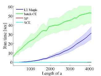
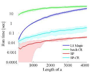
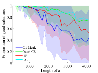
Figure 1: Performance and run time of different sparse coding methods as a function of the size of the representation. Compared methods: $l_{1}$-Magic, (batch) CE, SP and subspace CE (SCE). (a)-(b) Average run time for the different methods as a function of overcompleteness, i.e. the size of the internal representation on linear and logarithmic plots, respectively. Size of input: $\dim(\mathbf{x})=64$, number of active components: $K=8$. (c) Ratio of good solutions (ratio of found good components) as a function of overcompleteness. Note: $l_{1}$-norm and SP methods used the correct number of non-zero components. The strict value of this number is not needed for CE and SCE methods

On Fig. 1 three graphs are shown to characterize the performance of $l_{1}$-Magic, SP, CE and SCE algorithms. Note that CE should find the optimal solution if allowed to run long enough. This is not the case for $l_{1}$-Magic and SP. Conditions of the theorems of $l_{1}$-Magic are roughly as follows [4]: solution can be found provided that the dimension of the input is larger than a constant (on the order of 4) multiplied with the number of non-zero coefficients and the logarithm of the size of the representation. Note that the condition may be spoiled by increasing the size of the internal representations. SP, for large representations, may be stuck in local minima, since it halts if reconstruction error is not improved at a given iteration. Last, but not least, both $l_{1}$-Magic and SP assume that the number of non-zero components is given beforehand, which is not needed for CE and SCE.

The first and second subplots (Fig. 1 and Fig. 1) show the mean ($\pm$std) run time on linear and logarithmic scales, respectively, as a function of the size of the internal sparse representation. The logarithmic scale shows the fine structure of the dependencies, but deviations get distorted. The linear scale demonstrates the order differences among the methods and also shows the symmetric deviation around the mean. The third plot (Fig. 1) depicts the ratio of good solutions as a function of the size of the internal sparse representation. The different methods fail to provide good solutions if they reach the maximum iteration number without converging to a solution or converge into an incorrect solution. Quite remarkably all methods show graceful degradation of performance even for internal dimensions on the order of 1,000. Nonetheless, there are clear advantages for the CE based methods for very sparse representations: SP and $l_{1}$-Magic methods reach ‘critical sparseness’ [10] much earlier. The SCE/CE advantage could be further increased by allowing longer iterations.

The reconstruction performance of SCE is the same as that of CE within measurement error. However, SCE runs orders of magnitudes faster than CE and $l_{1}$-magic. The speed of SCE is due to two factors. One factor is that SCE is using relatively few time consuming bottom-up transformations. The other factor is the principled introduction of mutual influence between the probability update of the individual components that incorporates the advantages of the SP method. In comparison with pure SP, SCE is only an order of magnitude slower than SP. Nevertheless, we expect to see further acceleration by extending the algorithm with a predictive module utilizing the CE probabilities not accessible by the pure SP.

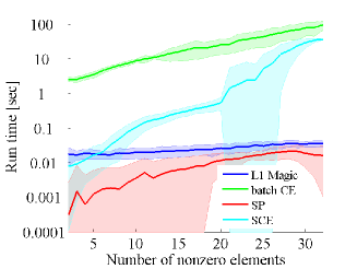
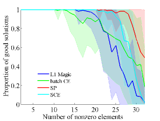
Figure 2: Performance and run time of different sparse coding methods as a function of the number of non-zero elements of the representation. Compared methods: $l_{1}$-Magic, (batch) CE, SP and subspace CE (SCE). (a) Run time for the different methods as a function of sparseness, i.e. the number of non-zero elements of the internal representation. Size of input: $\dim(\mathbf{x})=64$, size of the overcomplete representation: $\dim(\mathbf{a})=1024$. (b) Ratio of good solutions (reconstruction quality) as a function of overcompleteness. Note: $l_{1}$-norm and SP methods used the correct number of non-zero components. The strict value of this number is not needed for CE and SCE methods

The impact of complexity on the different methods has been tested by changing the number of non-zero components in the overcomplete representations. Figure 2 summarizes the results. Here again the running time (Fig. 2) and the ratio of good solutions (Fig. 2) are plotted, but now as a function of the number of non-zero components. In this test SP seems superior, but the combined method still performs well (increased number of iterations would allow even better performance at the price of longer run time). Furthermore as the divergence ratio (size of internal representation/size of input) increases, SP requires increasingly more iteration for calculating the reconstruction error, thus resulting in an enormous number of additional synaptic transmissions. This disadvantage does not show up in runtime using Matlab on a single PC since Matlab is optimized for matrix-vector computations. Let us remark that performance of SP may quickly deteriorates if the number of non-zero components is not known beforehand, which is the typical case in real scenarios.

4 Discussion

According to the expectations brain inspired computations are going to dominate and shape technology in the near future. While the most compelling features of neural systems are 1) the extremely low energy cost, 2) massively parallel and distributed organization and 3) outstanding resilience (robustness against structural and functional perturbations, self-organizing mechanisms for self-repair, etc), mainstream digital solutions mostly focus on speed, are organized in a serial fashion and even small scale perturbations can make them malfunction or totally dysfunctional. In order to make a paradigm shift, we need to have a better understanding of the structural and functional constituents of the neural systems responsible for the development and maintenance of these features. In this article we presented a very efficient signal processing approach designed to form overcomplete, sparse representations. In theoretical neuroscience the usefulness of such representations has long been recognized (e.g. [37]) for its contribution to increased storage capacity, better pattern separation and higher noise tolerance.

Recent discoveries in signal processing now suggest another important factor that must be utilized by evolutionary solutions as well. For most natural signals (i.e. those that are encountered most frequently by living systems) very efficient sampling is possible by exploiting their intrinsic sparseness. The fact that signals can be recovered by a small set of samples has serious impact on computational speed as well as on noise tolerance since even partially observed signals can also be recovered. A few novel models [43, 9, 45] have already started to implement these ideas in neural computations. These studies either deal with learning efficient dictionaries (in terms of reconstruction quality) or draw parallels between sensory processing and compressed sensing [13, 4]. In this article we argued that efficiency in terms of metabolic cost should also be taken into account when considering sparse coding mechanisms. Since this constraint is equally important for artificial and natural systems we wanted to improve $l_{1}$-norm based solutions by explicitly minimizing the required number of signal transmission (e.g. by reducing the number of signal projections and comparisons, especially when bottom-up transmissions are needed). In contrast to $l_{1}$-norm based methods, our solution, which is designed to explicitly minimize the active number of components (i.e., the $l_{0}$ norm), can be efficiently implemented in a parallel, distributed system. Furthermore, the CE method ensures convergence to the optimal solution [47, 31], which may not be the case for $l_{1}$-norm based solutions if conditions are not met. What is remained to answer is whether the SCE algorithm can be implemented in a neurally plausible form.

4.1 Neural plausibility of the SCE method

To discuss whether our algorithm makes sense in neural terms, implementation and functional issues need to be considered. As the implementation is concerned, although a detailed translation of the model into equations used by computational neuroscience is missing, we conjecture that SCE with online CE [25] can be expressed in neuronal form. An important property of the online variant of CE is that it preserves the convergence properties of the original batch method [55] although it relies on threshold adaptation and needs to identify elite samples and update the probabilities at each iteration. Since thresholds of individual neurons and neuronal ensembles can be independently and locally adapted and the discrete time updates of the algorithm can be rephrased in differential forms similar to those describing the changes of membrane potential we believe that the whole procedure can be translated into neuronal form.

As it was demonstrated our solution is indeed a very efficient sparse coding solution with local rules supporting distributed implementations. However, SP based update, while considerably accelerating the computations, does not seem to support lifetime sparseness (at least transiently). This shortcoming may, for example, be compensated by feedforward inhibitory thresholding [45].

$k$-WTA is another algorithmic component of our computations. In SCE, its role is to keep the number of active components low and to update the probabilities of the components. WTA methods have been already proposed as a computational primitive in the neural system On a particular use of $k$-WTA in modeling the hippocampal computations, see [40], whereas for a recent paper on the computational power of neural WTA methods, see, e.g., [27].

The proposed algorithm uses two distinct quantities: the probability of firing (feature selection) and the activity that reconstructs the input (coefficients of the features). Whether this dichotomy can be mapped onto assumed forms of neural computations is an open question. There are many potential solutions, ranging from local neuronal circuits, through considerations on population codes [41, 26] to models that neurons themselves represent multi-layer networks exhibiting a range of linear and non-linear mechanisms [24]. Future work will focus on this issue.

It has been long debated if the nature of neocortical sensory processing is mostly feedforward or feedback, since even the first spikes after stimulus onset may carry enough information in e.g. recognition tasks. [57]. While most arguments are about the expected speed of information processing, the capacity of the generative networks or the impact of anatomical and physiological constraints (see, e.g., [42, 19, 51, 50, 22]), we find that a particular combination of feedforward (bottom-up) and feedback (top-down) processing provides the most favorable solution for sparse coding in terms of metabolic cost. Given that the statistics of natural signals supports sparse representations, ecological solutions, like this combined process, may have evolutionary advantage over purely feedforward or feedback solutions.

In respect to the criticisms of [45] against previously proposed neural sparse coding mechanisms our solution 1) is neurobiologically plausible (using decentralized and local interactions at low synaptic activity), 2) can generate exactly zero-valued coefficients (since it directly minimizes the number of active components) and 3) it is based on a principled approach as opposed to heuristic approximations applied in other proposals. However, the $4^{th}$ issue about non-smooth variations in the coefficients for time-varying stimuli has not yet been addressed. Its importance stems from the belief that prediction is probably the most fundamental task of the neural system [23]. Hence any model claiming to explain some aspects of neural representation should provide means to support this central task. Currently we are seeking methods to make the proposed algorithm applicable for predicting time-varying sparse signals. Future work will show if the emerging probabilistic representations can be used e.g. in a belief propagation network thus supporting prediction.

Because all algorithmic steps can be realized by local interactions keeping a low energy profile, we argue that the emerging architecture might be a good model of neural sparse coding in sensory information processing. Although the generation of candidate representations and the update of the component probabilities require recurrent interactions, the constraint to minimize reentrant activity (i.e. reducing the intra-layer synaptic activity) results in apparent and approximately correct fast feed-forward working.

Beyond the low metabolic costs of the proposed algorithm, the $l_{0}$-norm based optimization provides additional flexibility over simple $l_{1}$-norm optimizations by not fixing the number of active components beforehand. Methods based on the $l_{1}$-norm (like SP) may fail if the optimal sparsity for a given stimuli differs from the predefined value. We note that for all tests $l_{1}$-norm based optimization schemes would have provided very poor approximations had they been restricted to keep a single ratio of non-zero components and the size of the representation (Fig. 1) or to keep a single number of non-zero components (Fig. 2).

5 Conclusions

We have proposed a novel solution for sparse coding by combining our previous work [25] on spike based probabilistic optimization using $l_{0}$-norm with an efficient $l_{1}$-norm based method. The motivation behind this integration is that $l_{1}$-norm based methods are computationally attractive and also provide the optimal solution under certain conditions [13, 5] while our $l_{0}$-norm based solution using the probabilistic cross-entropy method provides a potential neural interpretation and does not require the exact knowledge of the number of non-zero components.

The combined method has several outstanding features making it an interesting candidate for neural sparse coding in the sensory systems: computations are local, distributed and ‘transmission efficient’ with low metabolic cost. In addition, the algorithm is less affected by constraints of other alternatives based on $l_{1}$-norm optimization.

6 Acknowledgement

Thanks are due to Zoltán Szabó for his helpful comments on the manuscript. This research has been partially supported by the EC NEST ‘Percept’ grant under contract 043261.

7 Appendix

7.1 Pseudocode for Subspace Pursuit

  

input:
	$\kappa=K/M$, $\mathbf{x}\in\mathbf{R}^{N}$			% sparsity and signal
	$t_{SP}$			% max iteration number
	$\mathbf{D}\in\mathbb{R}^{N\times M}$			% $M$ element dictionary
initialization:
	$\mathcal{K}=\verb"MaxInd"_{\mathcal{K}}(\mathbf{D}^{T}\mathbf{x})$			% index set of size $K$
	$\mathbf{D}=\mathbf{D}[\mathcal{K}]$			% $K$-truncated matrix
	$\mathbf{r}\leftarrow\mathbf{x}-\mathbf{D}\mathbf{D}^{{\dagger}}\mathbf{x}$			% compute residual
optimization:
	for $t$ from $1$ to $t_{SP}$			% iteration main loop
		$\verb"compute "\mathcal{K}[\mathbf{D}^{T}\mathbf{r}]$		% index set for expansion
		$\mathcal{L}\leftarrow\mathcal{K}\cup\mathcal{K}[\mathbf{D}^{T}\mathbf{r}]$		% increase set size ($L=2K$)
		$\mathbf{e}\leftarrow\mathbf{D}[\mathcal{L}]^{{\dagger}}\mathbf{x}$		% compute projections
		$\mathcal{K}\leftarrow\verb"MaxInd"_{\mathcal{K}}(\mathbf{e})$		% new index set of size $K$
		$\mathbf{D}\leftarrow\mathbf{D}[\mathcal{K}]$		% $K$-truncated matrix
		$\mathbf{r}t\leftarrow\mathbf{x}-\mathbf{D}\mathbf{D}^{{\dagger}}\mathbf{x}$		% compute residual
		$\verb"if "\mathbf{r}^{t}=0\verb" then quit"$		% finish is residual is zero
		$\verb"if "\|\mathbf{r}^{t}\|_{2}\geq\|\mathbf{r}^{t-1}\|_{2}\verb" then"$		% check for improvement
			$t=t_{SP}$	% no new iteration
			$\mathcal{K}^{t_{SP}}=\mathcal{K}^{t-1}$	% use previous index set
		$\verb" quit"$
	end loop

  

Table 3: The pseudocode of the Subspace Pursuit method of [10]. The significant difference between this and other iterative MP methods is the refinement of the already chosen subset of basis by testing the projection of the original signal onto the current basis set.

7.2 CE method for Bernoulli distribution

Let the domain of optimization be $\mathbf{y}\in\mathscr{Y}=\{0,1\}^{M}$, and each component be drawn from independent Bernoulli distributions, i.e., ${\mathcal{G}}=\textit{BER}\/^{M}$. Each distribution $g\in\mathcal{G}$ is parameterized with an $M$-dimensional vector $\mathbf{p}=(p_{1},\ldots,p_{M})$. Component $j$ of the sample $\mathbf{y}\in\mathbf{y}\in\mathscr{Y}$ drawn from distribution $g$ thus will be

$$y_{j}=\left\{\begin{array}[]{ll}1,&\hbox{with probability $p_{j}$;}\\ 0,&\hbox{with probability $1-p_{j}$.}\\ \end{array}\right.$$

Having drawn $I$ samples $\mathbf{y}^{(1)},\ldots,\mathbf{y}^{(I)}$, let $L_{\gamma}$ denote the level set of the elite samples, i.e.,

$$L_{\gamma}:=\{\mathbf{y}^{(i)}\mid f(\mathbf{y}^{(i)})\leq\gamma\}$$

where $\gamma$ denotes a fixed threshold value. The distribution $g^{\prime}$ with minimum cross-entropy distance from the uniform distribution over the elite set has the following parameters [11]:

$$\mathbf{p}^{\prime} := (p^{\prime}_{1},\ldots,p^{\prime}_{M}),\quad\textrm{where}$$

$$p^{\prime}_{j} := \frac{\sum_{\mathbf{y}^{(i)}\in L_{\gamma}}\chi(y^{(i)}_{j}\!=\!\,\,1)}{\sum_{\mathbf{y}^{(i)}\in L_{\gamma}}1}=\frac{\sum_{\mathbf{y}^{(i)}\in L_{\gamma}}\chi(y^{(i)}_{j}\!=\!1)}{\rho\cdot I}$$ (7.1)

where $\chi(.)$ is an indicator function. In other words, the parameters of $g^{\prime}$ are simply the componentwise empirical probabilities of 1s in the elite set. Changing the distribution parameters from $\mathbf{p}$ to $\mathbf{p}^{\prime}$ can be too coarse, so in some cases, applying a step-size parameter $\alpha$ is preferable. The resulting algorithm is summarized in Table 4.

  

required:
	$\mathbf{p}=(p_{1},\ldots,p_{M})$			% initial distribution parameters
	$T$,			% max iteration number
	$I$			% population size,
	$\rho$			% selection ratio
	for $t$ from $1$ to $T$			% CE iteration main loop
		for $i$ from $1$ to $I$
			draw $\mathbf{y}^{(i)}$ from $\textit{BER}^{M}(\mathbf{p}_{t})$	% draw $I$ samples
			compute $f^{i}:=f(\mathbf{y}^{(i)})$	% evaluate them
		sort $f^{i}$-values		% order by decreasing magnitude
		$\gamma\leftarrow f_{\rho\cdot I}$		% level set threshold
		$L_{\gamma}\leftarrow\{\mathbf{y}^{(i)}\mid f(\mathbf{y}^{(i)})\leq\gamma\}$		% get elite samples
		$p^{\prime}_{j}\leftarrow\bigl{(}\sum_{\mathbf{y}^{(i)}\in L_{\gamma}}\chi(y^{(i)}_{j}\!=\!\,\,1)\bigr{)}/(\rho\cdot I)$		% get parameters of nearest distrib.
		$p_{j}\leftarrow\alpha\cdot p^{\prime}_{j}+(1-\alpha)\cdot p_{j}$		% update with step-size $\alpha$
	end loop

  

Table 4: Pseudo-code of the cross-entropy method for Bernoulli distributions

References

- [1] G. Allon, Dirk P. Kroese, T. Raviv, and Reuven Y. Rubinstein. Application of the cross-entropy method to the buffer allocation problem in a simulation-based environment. Annals of Operations Research, 134:137–151, 2005.
- [2] Pietro Berkes, Ben White, and Jozsef Fiser. No evidence for active sparsification in the visual cortex. In Y. Bengio, D. Schuurmans, J. Lafferty, C. K. I. Williams, and A. Culotta, editors, Advances in Neural Information Processing Systems 22, pages 108–116, 2009.
- [3] S. Boyd and L. Vandenberghe. Convex Optimization. Cambridge University Press, 2004.
- [4] E. Candès, J. Romberg, and T. Tao. Robust uncertainty principles: exact signal reconstruction from highly incomplete frequency information. IEEE Trans. Inf. Theory, 52:489–509, 2006.
- [5] W. Candès and J. Romberg. -magic: A collection of matlab routines for solving the convex optimization programs central to compressive sampling. online, 2006. http://www.acm.caltech.edu/l1magic/.
- [6] G. A. Carpenter and S. Grossberg. ART2: self-organization of stable category recognition codes for analog input patterns. Applied Optics, 26:4919–4930, 1987.
- [7] G.A. Carpenter and S. Grossberg. A massively parallel architecture for a self-organizing neural pattern recognition machine. Computer Vision, Graphics, and Image Processing, 37:54–115, 1987.
- [8] S. Chen, D. Donoho, and M. Saunders. Atomic decomposition by basis pursuit. SIAM Journal on Scientific Computing, 43(1):129–159, 2001.
- [9] W. K. Coulter, C. J. Hillar, G. Isely, and F. T. Sommer. Adaptive compressed sensing - a new class of self-organizing coding models for neuroscience. accepted at ICASSP2010, 2010. http://www.msri.org/people/members/chillar/files/ACS-ICASSP10.pdf.
- [10] W. Dai and O. Milenkovic. Subspace pursuit for compressive sensing signal reconstruction. IEEE Transactions on Information Theory, 55(5):2230–2249, 2009.
- [11] Pieter-Tjerk de Boer, Dirk P. Kroese, Shie Mannor, and Reuven Y. Rubinstein. A tutorial on the cross-entropy method. Annals of Operations Research, 134:19–67, 2004.
- [12] D. Donoho, Y. Tsaig, I. Drori, and F. Starck. Sparse solution of underdetermined linear equations by stagewise orthogonal matching pursuit, 2006. Technical Report 2006-02,Stanford, CA: Stanford University.
- [13] D. L. Donoho. Compressed sensing. IEEE Transactions on Information Theory, 52:1289–1306, 2006.
- [14] D. J. Field. What is the goal of sensory coding. Neural Computation, 6:559–601, 1994.
- [15] F. Girosi. An equivalence between sparse approximation and support vector machines. Neural Computation, 10:1455–1480, 1998.
- [16] D. J. Graham and D. J. Field. Sparse coding in the neocortex. In Jon H. Kaas and Leah A. Krubitzer, editors, Evolution of Nervous Systems, volume III, pages 181–187. Elsevier, 2006.
- [17] Jonathan Keith and Dirk P. Kroese. Sequence alignment by rare event simulation. In Proceedings of the 2002 Winter Simulation Conference, pages 320–327, 2002.
- [18] S. Kim, K. Koh, M. Lustig, S. Boyd, and D. Gorinevsky. An interior-point method for large-scale l1-regularized logistic regression. Journal of Machine Learning Research, 2007, 2007.
- [19] C. Koch and T. Poggio. Predicting the visual world: silence is golden. Nature Neuroscience, 2:9–10, 1999.
- [20] H. Lee, A. Battle, R. Raina, and A. Y. Ng. Efficient sparse coding algorithms. In In NIPS, pages 801–808. NIPS, 2007.
- [21] P. Lennie. The cost of cortical computation. Current Biology, 13:493–497, 2003.
- [22] H. Liu, Y. Agam, J. R. Madsen, and G. Kreiman. Timing, timing, timing: Fast decoding of object information from intracranial field potentials in human visual cortex. Neuron, 62:281 290, 2009.
- [23] R. Llinas. I of the Vortex: From neurons to self. The MIT Press, 2002.
- [24] M. London and M. Häusser. Dendritic computation. Annu. Rev. Neurosci., 28:503 532, 2005.
- [25] A. Lőrincz, Zs. Palotai, and G. Szirtes. Spike-based cross-entropy method for reconstruction. Neurocomputing, 71:3635–3639, 2008.
- [26] W. J. Ma, J. M. Beck, P. E. Latham, and A. Pouget. Bayesian inference with probabilistic population codes. Nature Neuroscience, 9:1432–1438, 2006.
- [27] W. Maass. On the computational power of winner-take-all. Neural Computation, 12(11):2519–2535, 2000.
- [28] B. Mailhe, R. Gribonval, F. Bimbot, and P. Vandergheynst. A low complexity orthogonal matching pursuit for sparse signal approximation with shift-invariant dictionaries. In ICASSP’09, IEEE Int. Conf. on Acoustics, Speech and Signal Processing, April 2009.
- [29] J. Mairal, F. Bach, J. Ponce, and G. Sapiro. Online learning for matrix factorization and sparse coding. Journal of Machine Learning Research, 11:19–60, 2010.
- [30] S. Mallat and Z. Zhang. Matching pursuits with time-frequency dictionaries. IEEE Transactions on Signal Processing, 41(12):3397–3415, 1993.
- [31] Heinz Muehlenbein. The equation for response to selection and its use for prediction. Evolutionary Computation, 5:303–346, 1998.
- [32] D. Mumford. Neuronal architectures for pattern-theoretic problems. In C. Koch and J. L. Davis, editors, Large Scale Neuronal Theories of the Brain, pages 125–152. MIT Press, 1994.
- [33] B. Natarajan. Sparse approximate solutions to linear systems. SIAM Journal on Computing, 24(2):227–234, 1995.
- [34] D. Needell and J. A. Tropp. Cosamp: Iterative signal recovery from incomplete and inaccurate samples. Appl. Comp. Harmonic Anal, 26:301–321, 2008.
- [35] D. Needell and R. Vershynin. Uniform uncertainty principle and signal recovery via regularized orthogonal matching pursuit. Foundations of Computational Mathematics, 9:317–334, 2009.
- [36] B. A. Olshausen. Sparse codes and spikes. In R. P. N. Rao, B. A. Olshausen, and M. S. Lewicki, editors, Probabilistic Models of the Brain: Perception and Neural Function, pages 257–272. MIT Press, 2002.
- [37] B. A. Olshausen and D. J. Field. Emergence of simple-cell receptive field properties by learning a sparse code for natural images. Nature, 381:607–609, 1996.
- [38] B. A. Olshausen and D. J. Field. Sparse coding with an overcomplete basis set: A strategy employed by V1? Vision Research, 37:3311–3325, 1997.
- [39] B. A. Olshausen and D. J. Field. Sparse coding of sensory inputs. Current Opinion in Neurobiology, 14:481–487, 2004.
- [40] R.C. O’Reilly and J.L. McClelland. Hippocampal conjunctive encoding, storage, and recall: Avoiding a tradeoff. Hippocampus, 4:661–682, 1994.
- [41] A. Pouget, P. Dayan, and R. Zemel. Information processing with population codes. Nature Reviews of Neuroscience, 1:125–132, 2000.
- [42] R. P. N. Rao and D. H. Ballard. Predictive coding in the visual cortex: A functional interpretation of some extra-classical receptive-field effects. Nature Neurosci., 2:79–87, 1999.
- [43] M. Rehn and F. T. Sommer. A network that uses few active neurones to code visual input predicts the diverse shapes of cortical receptive fields. Journal of Computational Neuroscience, 22:135–146, 2007.
- [44] M. Riesenhuber and T. Poggio. Hierarchical models of object recognition in cortex. Nature Neuroscience, 2:1019–1025, 1999.
- [45] C. J. Rozell, D. H. Johnson, E. G. Baraniuk, and B. A. Olshausen. Sparse coding via thresholding and local competition in neural circuits. Neural Computation, 20(10):2526–2563, 2008.
- [46] R. Rubinstein and D. P. Kroese. The Cross-Entropy Method. Springer-Verlag, New York, 2004.
- [47] R. Y. Rubinstein. The cross-entropy method for combinatorial and continuous optimization. Methodology and Computing in Applied Probability, 2:127–190, 1999.
- [48] F. Santosa and W. W. Symes. Linear inversion of band-limited reflection seismograms. SIAM J. Sci. and Stat. Comput., 7:1307–1330, 1986.
- [49] M. Seeger. Bayesian inference and optimal design in the sparse linear model. Journal of Machine Learning Researc, 9:759–813, 2008.
- [50] T. Serre, A. Oliva, and T. Poggio. A feedforward architecture accounts for rapid categorization. Proceedings of the National Academy of Science, 104:6424 6429, 2007.
- [51] A. M. Sillito, J. Cudeiro, and H. E. Jones. Always returning: feedback and sensory processing in visual cortex and thalamus. Trends in Neurosciences, 29:307 – 316, 2006.
- [52] E. C. Smith and M. S. Lewicki. Efficient auditory coding. Nature, 439:978–982, 2006.
- [53] Z. Szabó, B. Póczos, and A. Lőrincz. Cross-entropy optimization for independent process analysis. In Justinian Rosca, Deniz Erdogmus, José C. Principe, and Simon Haykin, editors, Independent Component Analysis and Blind Signal Separation, volume 3889 of Lecture Notes in Computer Science, pages 909–916. Springer, 5-8 March 2006.
- [54] I. Szita and A. Lőrincz. Learning to play using low-complexity rule-based policies: Illustrations through Ms. Pac-Man. Journal of Artificial Intelligence Research, 30:659–684, 2007.
- [55] I. Szita and A. Lőrincz. Online variants of the cross-entropy method, 2008. http://arxiv.org/abs/0801.1988.
- [56] T. Tao. Preprints in sparse recovery /compressed sensing, 2008. http://www.math.ucla.edu/~tao/preprints/sparse.html.
- [57] S. J. Thorpe. How can the human visual system process a natural scene in under 150ms? Experiments and neural network models. In Michel Verleysen, editor, Eurorean Symposium on Artificial Neural Networks. D-Facto public, 1997.
- [58] J. A. Tropp. Greed is good: algorithmic results for sparse approximation. IEEE Transactions on Information Theory, 50(10):2231–2242, 2004.
- [59] W. Vinje and J. Gallant. Natural stimulation of the nonclassical receptive field increases information transmission efficiency in v1. Journal of Neuroscience, 22:2904–2915, 2002.
- [60] Y. Weiss, H. Chang, and W. Freeman. Learning compressed sensing, 2007. (in press) http://www.cs.huji.ac.il/~yweiss/allerton-final.pdf.
- [61] B. Willmore and D. Tolhurst. Characterising the sparseness of neural codes. Network: Comput. Neural Syst, 12:255–270, 2001.