Numerical shadows: measures and densities on the numerical range

Abstract

For any operator $M$ acting on an $N$-dimensional Hilbert space ${\cal H}_{N}$ we introduce its numerical shadow, which is a probability measure on the complex plane supported by the numerical range of $M$. The shadow of $M$ at point $z$ is defined as the probability that the inner product $(Mu,u)$ is equal to $z$, where $u$ stands for a random complex vector from ${\cal H}_{N}$, satisfying $||u||=1$. In the case of $N=2$ the numerical shadow of a non-normal operator can be interpreted as a shadow of a hollow sphere projected on a plane. A similar interpretation is provided also for higher dimensions. For a hermitian $M$ its numerical shadow forms a probability distribution on the real axis which is shown to be a one dimensional $B$-spline. In the case of a normal $M$ the numerical shadow corresponds to a shadow of a transparent solid simplex in ${\mathbb{R}}^{N-1}$ onto the complex plane. Numerical shadow is found explicitly for Jordan matrices $J_{N}$, direct sums of matrices and in all cases where the shadow is rotation invariant. Results concerning the moments of shadow measures play an important role. A general technique to study numerical shadow via the Cartesian decomposition is described, and a link of the numerical shadow of an operator to its higher-rank numerical range is emphasized.
AMS classification:  47A12, 60B05, 81P16, 33C05, 51M15

I Introduction

The classical numerical range $W(M)$ of a complex $N\times N$ matrix $M$ is the subset of ${\mathbb{C}}$ defined by

$$W(M)=\{(Mu,u):u\in{\mathbb{C}}^{N},\|u\|=1\}.$$

This concept has a long history and has proved a useful tool in operator theory and matrix analysis as well as in more applied areas; for a nice account of some of the lore of $W(M)$, see [GR1997]. Here we are concerned with the measures or densities induced on $W(M)$ by various distributions of the unit vector $u$; we use the term numerical shadow to refer to such densities (see section 2 for our motivation in using this terminology). Although it seems natural to study the numerical shadow, this subject does not seem to have received much attention until recently. The only earlier extended account (that we know of) is the thesis [N1982]. This apparent neglect is not the only reason for our attempts to understand the numerical shadow better; the numerical shadow also plays an interesting role in quantum information theory. Applications in this area are the focus of a companion paper [DGHMPŻ2], in preparation. Very recently a preprint by Gallay and Serre [GS2010] has appeared, dealing also with mathematical aspects of the numerical shadow (numerical measure, in their terminology). In several ways their development of the subject is parallel to our own (as presented, for example, in [Ż2009] and [H2010]). In the present paper we stress those aspects of our work which are complementary to [GS2010], particularly those based on the moments of the numerical shadow.
In this paper we work mainly with the “uniform” distribution of $u$ over the unit sphere $\Omega_{N}$ in ${\mathbb{C}}^{N}\equiv{\mathbb{R}}^{2N}$, ie the probability distribution on $\Omega_{N}$ that is invariant under all orthogonal transformations of ${\mathbb{R}}^{2N}$. In some cases, however, the internal structure of $W(M)$ is better revealed through the use of other distributions, and these are of special importance for the applications discussed in [DGHMPŻ2].
Although the numerical shadow is in general difficult to determine explicitly, this is possible in a number of interesting cases. Methods based on identifying the moments of the shadow measures are often effective. We also present, via the figures, the results of numerical simulations that display shadow densities in various other cases.
In section 2 we treat the simple situation occurring when $M$ is $2\times 2$. Here we obtain a “real–life” shadow. In section 3 we discuss the analogous treatment for $N\times N$ matrices $M$, ie we view the numerical shadow of $M$ as the image of an appropriate measure on the pure states $uu^{*}$ under a linear map ${\varphi}_{M}$. In section 4 we show that in the case of $N\times N$ normal $M$ the numerical shadow is the orthogonal projection of a well-placed model of the ($N-1$)–dimensional simplex (with the uniform density). Thus the density for the numerical shadow is a 2–dimensional B-spline (1-dimensional in the Hermitian case).
Section 5 studies the moments of numerical shadows, yielding a key technique for the identification and comparison of shadows. In section 6, criteria for the equality of the numerical shadows of two matrices are obtained (in terms, for example, of traces of words in the matrices and their adjoints). Evidently equality occurs when the matrices are unitarily equivalent, but this is not necessary (if $N>2$).
In section 7, the numerical shadows are found explicitly for the Jordan nilpotents $J_{N}$. Section 8 extends the techniques developed in section 7 to obtain explicit densities for all rotation invariant shadows.
Section 9 introduces a useful view of the numerical shadow in terms of the (Hermitian) components Re($M$) and Im($M$) in the Cartesian decomposition of $M$, and the unitary matrix linking those components. Several related aspects of the numerical shadow are treated in that section, including a connection with the Radon transform. Section 10 relates the numerical shadow of a direct sum to the shadows of its summands. Section 11 is concerned with numerical approximations of shadow densities in terms of moments and Zernike expansions.
Finally, in section 12, we relate the numerical shadow of $M$ to the so–called rank–$k$ numerical ranges $\Lambda_{k}(M)$. The theory and applications of these ranges has been advanced vigorously since their introduction only a few years ago as a tool in quantum information theory (see for example [CKŻ2006a, CKŻ2006b, CHKŻ2007, CGHK2008, W2008, LS2008, LPS2009, and GLW2010]). One way to describe $\Lambda_{k}(M)$ is that it consists of those points $(Mu,u)$ in $W(M)$ where $u$ may be chosen from the unit sphere in a whole $k$–dimensional subspace of ${\mathbb{C}}^{N}$. Thus it is natural to ask to what extent $\Lambda_{k}(M)$ may be identified as a region of greater density within the numerical shadow. Here the shadows corresponding to real unit vectors $u$ play a role.
Let us fix some notation. The algebra of complex $N\times N$ matrices is here denoted by $M_{N}({\mathbb{C}})$ or simply $M_{N}$. The adjoint or conjugate transpose of a matrix $M\in M_{N}$ is denoted by $M^{*}$; we consider vectors $v$ in ${\mathbb{C}}^{N}$ as column vectors and $v^{*}$ is the conjugate transpose. Our inner product $(v,w)$ may be computed as $w^{*}v$. Recall that the unit sphere in ${\mathbb{C}}^{N}$ is denoted by $\Omega_{N}$, ie

$$\Omega_{N}=\{u\in{\mathbb{C}}^{N}:\|u\|=1\}.$$

The uniform probability measure on $\Omega_{N}$ is denoted by $\mu$. Given $M\in M_{N}$, the notion of “numerical shadow of $M$” is captured formally as the probability measure $P_{M}$ on $W(M)$ such that

$$P_{M}(S)=\mu\{u\in\Omega_{N}:(Mu,u)\in S\},$$

for each Borel subset $S$ of $W(M)$. Equivalently, for any continuous function $g:W(M)\to{\mathbb{C}}$ we have

$${\int_{W(M)}g(z)\,dP_{M}(z)=\int_{\Omega_{N}}g((Mu,u))\,d\mu(u).}$$ (1)

If $P_{M}$ has a probability density (with respect to planar measure in ${\mathbb{C}}$) it is denoted by $f_{M}$. In those cases where $f_{M}$ is rotation–invariant, ie $f_{M}(z)=f_{M}(|z|)$ we consider $f_{M}$ as a function of $r\in(0,w(M))$, where $w(M)$ is the so–called numerical radius of $M$:

$$w(M)=\max\{|z|:z\in W(M)\}.$$

Acknowledgements: Work by J. Holbrook was supported in part by an NSERC of Canada research grant. Work by P. Gawron and Z.Puchała was supported by the Polish Ministry of Science and Higher Education under the grant number N519 442339, while K. Życzkowski acknowledges support by the grant number N202 090239.

Contents

1. I Introduction
2. II The $2\times 2$ case; real–life shadows
3. III Numerical shadows as linear images of the pure quantum states
4. IV The Hermitian and normal cases: B–splines
5. V Moments of the numerical shadow
6. VI Criteria for equality of numerical shadows
7. VII Numerical shadows of Jordan nilpotents $J_{N}$
8. VIII Rotation–invariant shadows
9. IX Numerical shadows via the Cartesian decomposition
   1. IX.1 Marginal densities
   2. IX.2 The shadow of a Hermitian matrix
   3. IX.3 The critical curves in W(A)
   4. IX.4 A geometric approach
   5. IX.5 Examples
10. X Direct sums (block diagonal matrices)
11. XI Zernike expansions
12. XII Numerical shadows and the higher–rank numerical ranges

II The $2\times 2$ case; real–life shadows

Here we compute the shadow density for an arbitrary $2\times 2$ matrix $M$. Our method is to view this density as a real–life shadow of the Bloch sphere model for $\Omega_{2}$. An equivalent result was obtained by Ng (see [N1982]) by a rather different method.
The Bloch sphere model sees $W(M)$ as the genuine shadow of a hollow sphere made of infinitely thin semi–transparent uniform material, where in general the light would fall obliquely on the (complex) plane. Of course, this situation cannot quite be realized physically, but playing with a hollow plastic ball in bright sunlight may yield a good approximation. It is well–known that when $M\in M_{2}$ the numerical range $W(M)$ is a filled ellipse with the eigenvalues of $M$ as foci. The following proposition, visualized in Fig. LABEL:fig:nonnormal2, supplies further information in the form of an explicit shadow density.
Proposition 2.1: Let $E$ be the filled ellipse formed by $W(M)$ and let $a$ and $b$ be the lengths of the semimajor and semiminor axes of $E$; then the shadow density is

$${\frac{1}{2\pi ab\sqrt{1-r^{2}}}}$$ (2)

at every point on the elliptical curve bounding $rE$ ($0\leq r\leq 1$).
Proof: Recall that we assume that $u$ is chosen “uniformly” over $\{u\in{\mathbb{C}}^{2}:\|u\|=1\}$, ie according to the measure $\mu$ on $\Omega_{2}$. It is known that $|u_{1}|^{2}$ will then be uniform in $[0,1]$. This a special case of the fact that $u$ uniform in $\Omega_{N}$ implies $(|u_{1}|^{2},|u_{2}|^{2},\dots,|u_{N}|^{2})$ has the uniform distribution in the $N-1$–dimensional simplex, see Ż (1999); BŻ (2006).

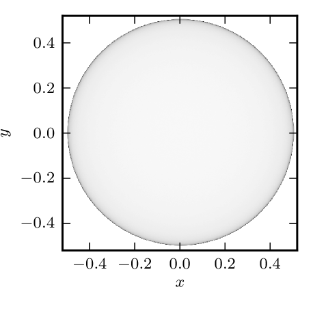
(a)

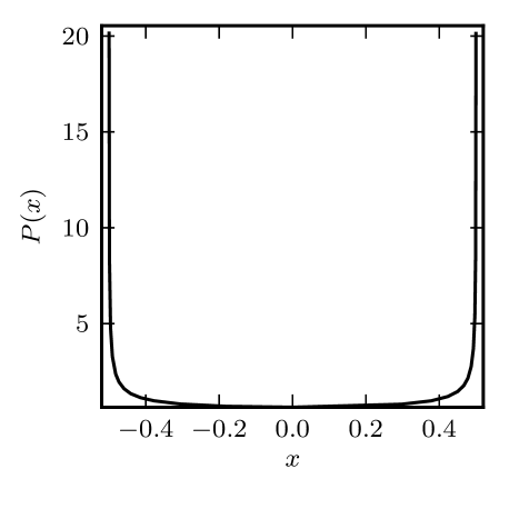
(b)

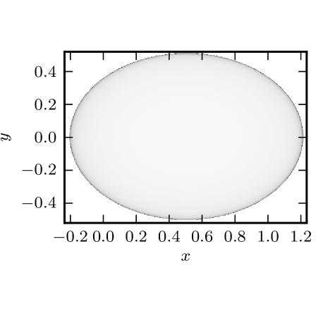
(c)

(d)

Figure 1:

It is also important to note that for fixed $u_{1}$ the relative phase of $u_{2}$ is $e^{i\theta}$ where $\theta$ is uniform in $[0,2\pi]$. We have

$$uu^{*}=\begin{bmatrix}|u_{1}|^{2}&u_{1}\overline{u_{2}}\\ \overline{u_{1}}u_{2}&|u_{2}|^{2}\end{bmatrix}=$$

$$\frac{1}{2}\begin{bmatrix}1&0\\ 0&1\end{bmatrix}+\frac{1}{2}\begin{bmatrix}2|u_{1}|^{2}-1&2u_{1}\overline{u_{2}}\\ 2\overline{u_{1}}u_{2}&1-2|u_{1}|^{2}\end{bmatrix}.$$

Let $z=2|u_{1}|^{2}-1$; then $z$ is uniform in $[-1,1]$ and $2u_{1}\overline{u_{2}}=\sqrt{1-z^{2}}e^{-i\theta}=x-iy$, so that (recalling Archimedes) $(x,y,z)$ is uniform on the unit sphere. This is one way to see that the corresponding distribution on the Bloch sphere $\{uu^{*}:u\in\Omega_{2}\}$ is uniform.
Following Davis [D1971], we compute $(Mu,u)$ as

$${\mbox{tr}}(u^{*}Mu)={\mbox{tr}}(Muu^{*})={\mbox{tr}}(\frac{1}{2}M+\frac{1}{2}M\begin{bmatrix}z&x-iy\\ x+iy&-z\end{bmatrix}).$$

For convenience we take $M=\begin{bmatrix}1&q\\ 0&-1\end{bmatrix}$ with $q\geq 0$. This is a harmless normalization, achieved via translation and rotation of $M$ (which respects the distribution of $(Mu,u)$) and unitary similarity (which leaves the distribution unchanged). Then $(Mu,u)=z+(q/2)(x+iy)=(z+bx,by)$ in the complex plane, with $b=q/2$. Consider the region $E$ bounded by the ellipse centred at $(0,0)$ with horizontal semiaxis of length $a=\sqrt{1+b^{2}}$ and vertical semiaxis of length $b$. Given $r\in[0,1]$, $(Mu,u)$ lies in $rE$ iff

$$\frac{(z+bx)^{2}}{1+b^{2}}+\frac{(by)^{2}}{b^{2}}\leq r^{2}.$$

A calculation verifies that this is equivalent to $((x,y,z)\cdot(1/a,0,-b/a))^{2}\geq 1-r^{2}$, saying that $(x,y,z)$ lies on either of the spherical caps of the unit sphere that are symmetrical about the axis determined by $(1/a,0,-b/a)$ and have radius $r$. According to Archimedes (or the related formulas found in calculus texts) the relative area of these caps is $1-\sqrt{1-r^{2}}$. Hence the probability

$$P((Mu,u)\in rE)=1-\sqrt{1-r^{2}}.$$

To find the corresponding planar density, we first observe that the region $(r+\Delta r)E\setminus rE$ corresponds to symmetrical rings bordering the spherical caps mentioned above. Thus the planar density will be constant on the ellipse bounding $rE$. Its value there is then given by

$$\lim_{\Delta r\to 0}\frac{(1-\sqrt{1-(r+\Delta r)^{2}})-(1-\sqrt{1-r^{2}})}{\pi ab(r+\Delta r)^{2}-\pi abr^{2}}=\frac{1}{2\pi ab\sqrt{1-r^{2}}}.$$

QED
This result is equivalent to the formula for the density obtained by Ng (see [N1982], page 67). He computes the density of $(Mu,u)$ at $(x,y)$ in the ellipse as

$$p(x,y)=\frac{1}{2\pi ab\sqrt{1-(x^{2}/a^{2}+y^{2}/b^{2})}}.$$

His method seems unrelated to the Bloch sphere approach worked out above.

III Numerical shadows as linear images of the pure quantum states

It is clear that the argument of section 2 can be extended in part to cases where $N>2$. The Bloch sphere is replaced by the set of density matrices representing pure quantum states:

$$PQS_{N}=\{uu^{*}:u\in\Omega_{N}\}.$$

Just as before, for any $u\in\Omega_{n}$ and $M\in M_{N}$ we have

$$(Mu,u)={\mbox{tr}}(u^{*}Mu)={\mbox{tr}}(Muu^{*}),$$

so that $W(M)$ is the image of $PQS_{N}$ under the linear map ${\varphi}_{M}:M_{N}\to{\mathbb{C}}$ defined by

$${\varphi}_{M}(X)={\mbox{tr}}(MX).$$

Since each $X\in PQS_{N}$ is Hermitian we may also write

$${\varphi}_{M}(X)={\mbox{tr}}(MX^{*})=(M,X)_{F},$$

where $(\cdot,\cdot)_{F}$ is the Frobenius inner product on $M_{N}$.
Thus the numerical shadow of $M$ may be viewed as the measure on $W(M)$ induced by applying the linear map ${\varphi}_{M}$ to the fixed measure $\nu$ on $PQS_{N}$ that corresponds to the uniform $\mu$ on $\Omega_{N}$. As $M$ varies the resulting numerical shadows may be regarded as a tomographic study of the measure $\nu$. Thus such detailed information as we have about numerical shadows (see section 9, for example, or [GS2010]) reveals much about the structure of $\nu$ on $PQS_{N}$.

IV The Hermitian and normal cases: B–splines

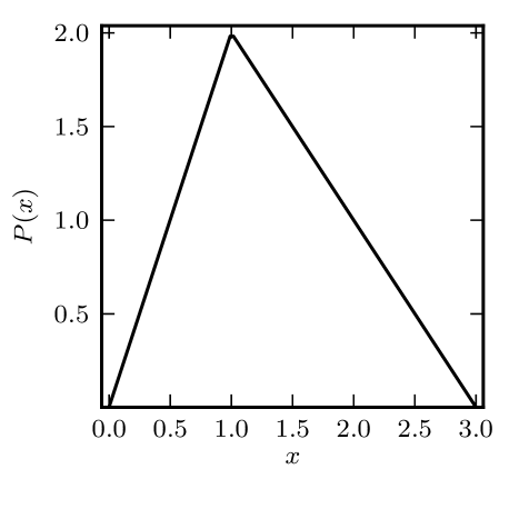
(a)

(b)

Figure 2: Probability density function of hermitian matrices of dimensions 3 and 4.

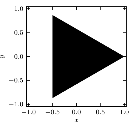
(a)

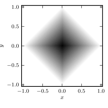
(b)

(c)

Figure 3: Probability density function of unitary matrices of dimensions 3, 4 and 5.

The standard $N$–simplex $\Delta_{N}$ is defined by

$$\Delta_{N}=\{r\in{\mathbb{R}}^{N}:\mbox{all }r_{k}\geq 0\mbox{ and }\sum_{k=1}^{N}r_{k}=1\}.$$

This is an ($N-1$)–dimensional convex subset of ${\mathbb{R}}^{N}$. We say $r$ is “uniformly distributed” over $\Delta_{N}$ to mean that $r$ is uniform with respect to normalized ($N-1$)–dimensional Lebesgue measure $vol_{N-1}$ on $\Delta_{N}$.
Lemma 4.1: Let $P_{A}$ be the shadow measure of a normal matrix $A\in M_{N}$. Then for any Borel subset $B$ of the plane

$$P_{A}(B)=\mbox{Prob}\{r^{*}{\lambda}\in B\},$$

where ${\lambda}=({\lambda}_{1},\dots,{\lambda}_{N})^{*}$ is the spectrum of $A$ and $r$ is uniformly distributed over the standard $N$–simplex $\Delta_{N}$.
Proof: Since $A$ is normal, it is unitarily similar to ${\mbox{diag}}({\lambda})$. As $\mu$ is invariant under unitary transformations we have

$$P_{A}(B)=\mbox{Prob}\{({\mbox{diag}}({\lambda})u,u)\in B:u\in\Omega_{N}\}=\mbox{Prob}\{(\sum_{k=1}^{N}{\lambda}_{k}|u_{k}|^{2}\in B:u\in\Omega_{N}\}.$$

It is known (see e.g. Ż (1999); BŻ (2006)) that if $u$ is uniform over $\Omega_{N}$ (ie distributed according to $\mu$) then

$$r=(|u_{1}|^{2},\dots,|u_{N}|^{2})$$

is uniform over the simplex $\Delta_{N}$. QED
With ${\lambda}$ as above, write ${\lambda}=x+iy$ where $x,y\in{\mathbb{R}}^{N}$. Assume first that $x$ and $y$ are independent vectors. Let $W$ be a real matrix with $x,y$ as its first two columns and with columns 3 to $N$ forming an orthonormal basis for $\{x,y\}^{\perp}$. For any vector $v\in{\mathbb{R}}^{N}$,

$$v^{*}{\lambda}=a+ib\,\,\,(a,b\in{\mathbb{R}})\quad\Leftrightarrow\quad(W^{*}v)_{1}=a\mbox{ and }(W^{*}v)_{2}=b.$$

Thus for Borel $B\subset{\mathbb{C}}\equiv{\mathbb{R}}^{2}$

$$\mbox{Prob}\{r^{*}{\lambda}\in B\}=vol_{N-1}\{r\in\Delta_{N}:((W^{*}r)_{1},(W^{*}r)_{2})\in B\},$$

and, in view of Lemma 4.1, the density for $P_{A}$ at $(a,b)\in W(A)$ is

$$vol_{N-3}\{r\in\Delta_{N}:(W^{*}r)_{1}=a,(W^{*}r)_{2}=b\}=vol_{N-3}\{v\in W^{*}(\Delta_{N}):v_{1}=a,v_{2}=b\}.$$

Let us recall the definition of an $s$–dimensional B–spline (from [dB1976]).
Definition 4.2: Let $\sigma$ be a nontrivial simplex in ${\mathbb{R}}^{s+k}$. On ${\mathbb{R}}^{s}$ we define the B–spline of order $k$ from $\sigma$ by

$$M_{k,\sigma}(x_{1},\dots,x_{s})=vol(\sigma\cap\{v\in{\mathbb{R}}^{s+k}:v_{j}=x_{j}\,\,(j=1,2,\dots,s)\}).$$

Using this terminology we may summarize our results as follows.
Proposition 4.3: The numerical shadow of an $N\times N$ normal matrix with eigenvalues ${\lambda}\in{\mathbb{C}}^{N}$ having linearly independent real and imaginary parts has as density a 2–dimensional B–spline $M_{N-2,\sigma}(a,b)$, where the simplex $\sigma=W^{*}(\Delta_{N})$ with some $W$ chosen as above.
Remark 4.4: In the case where the real and imaginary parts of ${\lambda}$ are dependent (as when $A$ is Hermitian), it is easy to see that the numerical shadow is 1–dimensional (a line segment, in fact) with density given by a 1–dimensional B–spline (compare [dB1976, Lemma 9.1]). As examples, the shadows of Hermitian matrices of size $N=3$ and $N=4$ are shown in Fig. 2.
Remark 4.5: This observation for the Hermitian case was worked out in detail by Ng in [N1982]. He also made the right conjecture regarding the normal case. In a sense, the normal case was earlier understood by statisticians studying the distribution of quadratic forms; see for example [A1971, chapter 6]; Anderson points out that some of the relevant ideas go back to von Neumann in the 40’s. Anderson seems to discuss only real quadratic forms; thus the normal case corresponds to roots of multiplicity 2.
Remark 4.6: In view of Proposition 4.3, the theory of B–splines may be applied to see that normal shadow densities are piecewise polynomial functions of two variables in the normal case - see Fig. 3 and of a single variable in the Hermitian case. The latter case is analyzed in some detail in Sec. 9. A thorough analysis of the B–spline shadow densities for normal matrices is also provided in [GS2010].

V Moments of the numerical shadow

We denote the moments of the numerical shadow of $A\in M_{N}$ by

$$\nu_{jk}(A)=\int_{W(A)}z^{j}\overline{z}^{k}\,dP_{A}(z).$$

Note that, since the polynomials in $z$ and $\overline{z}$ are uniformly dense in the continuous functions on $W(A)$, these moments determine the numerical shadow uniquely. Moreover, in view of (1), we have

$$\nu_{jk}(A)=\int_{\Omega_{N}}(Au,u)^{j}(\overline{(Au,u)})^{k}\,d\mu(u)=\int_{\Omega_{N}}(Au,u)^{j}(A^{*}u,u)^{k}\,d\mu(u).$$ (3)

Given ${\lambda}\in{\mathbb{C}}^{N}$ and a multi–index $\alpha\in{\mathbb{N}}_{0}^{N}$ (where ${\mathbb{N}}_{0}=\{0,1,2,\dots\}$), we use the following notation: ${\lambda}^{\alpha}={\lambda}_{1}^{\alpha_{1}}{\lambda}_{2}^{\alpha_{2}}\dots\lambda_{N}^{\alpha_{N}}$, $|\alpha|=\sum_{1}^{N}\alpha_{k}$, $\alpha!=\alpha_{1}!\alpha_{2}!,\dots\alpha_{N}!$. We also use the Pochhammer symbol or shifted factorial $(x)_{n}=\prod_{j=1}^{n}(x+j-1)$; by convention $(x)_{0}=1$.
The effective evaluation of the moments $\nu_{jk}(A)$ depends on the following proposition.
Proposition 5.1: Given $A\in M_{N}$, let ${\lambda}\in{\mathbb{C}}^{N}$ list the eigenvalues of $A$ repeated according to multiplicity. Then

$$\int_{\Omega_{N}}(Au,u)^{n}\,d\mu(u)=\frac{n!}{(N)_{n}}h_{n}({\lambda}),$$ (4)

where $h_{n}({\lambda})$ is the complete symmetric polynomial of degree $n$, ie

$$h_{n}({\lambda})=\sum_{\alpha\in{\mathbb{N}}_{0}^{N},\,\,|\alpha|=n}{\lambda}^{\alpha}.$$

Proof: Given multi–indices $\alpha,\beta$, let

$$Q(\alpha,\beta)=\int_{\Omega_{N}}u^{\alpha}(\overline{u})^{\beta}\,d\mu(u),$$ (5)

where the conjugation $\overline{u}$ is applied entrywise. Since $\mu$ is invariant under the unitary map $u\to(e^{i\theta}u_{1},u_{2},\dots,u_{N})^{t}$, we have $Q(\alpha,\beta)=e^{i(\alpha_{1}-\beta_{1})\theta}Q(\alpha,\beta)$ for each real $\theta$. Hence $Q(\alpha,\beta)=0$ unless $\alpha_{1}=\beta_{1}$. Similarly for the other components, so that $Q(\alpha,\beta)=0$ unless $\alpha=\beta$. More work is required to evaluate $Q(\alpha,\alpha)$:

$$Q(\alpha,\alpha)=\int_{\Omega_{N}}|u|^{2\alpha}\,d\mu(u)=\frac{\alpha!}{(N)_{|\alpha|}},$$ (6)

where $|u|=(|u_{1}|,|u_{2}|,\dots,|u_{N}|)^{t}$. A convenient trick here is to consider

$$I=\int_{{\mathbb{R}}^{2N}}e^{-\sum_{1}^{N}(x_{k}^{2}+y_{k}^{2})}\prod_{1}^{N}(x_{k}^{2}+y_{k}^{2})^{\alpha_{k}}\,\,dx\,dy.$$

As a product of Gamma–integrals we obtain $I=\pi^{N}\alpha!$. Integrating first over $r\Omega_{N}$, with $r^{2}=\sum_{1}^{N}(x_{k}^{2}+y_{k}^{2})$, then over $0<r<\infty$, we find that $I=\frac{1}{2}|S^{2N-1}|(N+|\alpha|-1)!Q(\alpha,\alpha)$, where $|S^{2N-1}|$ denotes the $(2N-1)$–dimensional area of $\Omega_{N}$. Since $Q(\vec{0},\vec{0})=1$, the formula (6) follows.
We may assume $A$ is in the Schur upper–triangular form, since this is obtained via a unitary similarity and $\mu$ is invariant under unitary transformations on ${\mathbb{C}}^{N}$. Thus $A_{jj}={\lambda}_{j}$ (some listing of the eigenvalues of $A$, with multiplicity) and

$$(Au,u)=\sum_{j=1}^{N}{\lambda}_{j}|u_{j}|^{2}+\sum_{j>i}A_{ij}u_{j}\overline{u_{i}}.$$

Aside from $(\sum_{j}{\lambda}_{j}|u_{j}|^{2})^{n}$, the terms of $(Au,u)^{n}$ are scalar multiples of expressions of the form

$$\prod_{k=1}^{a}|u_{\ell_{k}}|^{2}\prod_{k=1}^{b}u_{j_{k}}\overline{u_{i_{k}}},$$

where $b\geq 1$ and each $j_{k}>i_{k}$. Such an expression has the form $u^{\gamma}(\overline{u})^{\gamma}u^{\alpha}(\overline{u})^{\beta}$ where, using $e(j)$ as a temporary notation for the multi–index with 1 in the $j$–th position and 0’s elsewhere,

$$\alpha=\sum_{k=1}^{b}e(j_{k}),\quad\beta=\sum_{k=1}^{b}e(i_{k}).$$

Clearly $\alpha_{1}=0$ and for some first $k_{0}>1$ we have $\alpha_{k_{0}}>0$; hence $\beta_{k}>0$ for some $k<k_{0}$, so that $\alpha\neq\beta$. Thus $Q(\gamma+\alpha,\gamma+\beta)=0$ so that such terms make no contribution to the integral over $\Omega_{N}$. It follows that

$$\int_{\Omega_{N}}(Au,u)^{n}\,d\mu(u)=\int_{\Omega_{N}}(\sum_{j=1}^{N}{\lambda}_{j}|u_{j}|^{2})^{n}\,d\mu(u).$$

Using the multinomial formula and (6), this integral is

$$\sum_{\alpha\in{\mathbb{N}}_{0}^{N},\,\,|\alpha|=n}\frac{n!}{\alpha!}{\lambda}^{\alpha}Q(\alpha,\alpha)=\sum_{\alpha\in{\mathbb{N}}_{0}^{N},\,\,|\alpha|=n}\frac{n!}{\alpha!}{\lambda}^{\alpha}\frac{\alpha!}{(N)_{n}}$$

$$=\frac{n!}{(N)_{n}}\sum_{\alpha\in{\mathbb{N}}_{0}^{N},\,\,|\alpha|=n}{\lambda}^{\alpha}=\frac{n!}{(N)_{n}}h_{n}({\lambda}).$$

QED
It will be convenient to use the notation ${\lambda}(A)$ to denote any listing of the eigenvalues of $A$, repeated according to multiplicity. Applying (4) with $A$ replaced by $sA+tA^{*}$ ($t,s$ real) and recalling (3) we obtain

$$\sum_{j=0}^{n}\binom{n}{j}s^{j}t^{n-j}\nu_{j,n-j}(A)=\frac{n!}{(N)_{n}}h_{n}({\lambda}(sA+tA^{*})).$$ (7)

Moreover, the RHS of (7) may be evaluated in terms of traces of words in $A$ and $A^{*}$, using known relations Mac (1995) among $h_{n}({\lambda})$, the power sums

$$p_{j}({\lambda})=\sum_{k=1}^{N}{\lambda}_{k}^{j}$$

(these equal ${\mbox{tr}}(A^{j})$ if ${\lambda}={\lambda}(A)$), and the elementary symmetric polynomials

$$e_{j}({\lambda})=\sum_{1\leq i_{1}<i_{2}<\dots<i_{j}\leq N}{\lambda}_{i_{1}}{\lambda}_{i_{2}}\dots\lambda_{i_{j}}$$

(note that $e_{j}({\lambda})=0$ if $j>N$; by convention $e_{0}({\lambda})=1$). For $n\geq 1$ we have

$$e_{0}h_{n}-e_{1}h_{n-1}+e_{2}h_{n-2}\dots\pm e_{n}h_{0}=0$$ (8)

(by convention $h_{0}({\lambda})=1$) and

$$ne_{n}=p_{1}e_{n-1}-p_{2}e_{n-2}+\dots\pm p_{n}e_{0}.$$ (9)

For example, $h_{1}=p_{1}$ so that (7) implies

$$t\nu_{0,1}(A)+s\nu_{1,0}(A) = \frac{1}{N}p_{1}({\lambda}(sA+tA^{*}))=\frac{1}{N}{\mbox{tr}}(sA+tA^{*})$$

$$= \frac{1}{N}(t\,\,{\mbox{tr}}(A^{*})+s\,\,{\mbox{tr}}(A)).$$

Hence

$$\nu_{1,0}(A)=\frac{1}{N}{\mbox{tr}}(A)\mbox{ and }\nu_{0,1}(A)=\frac{1}{N}{\mbox{tr}}(A^{*}).$$

Likewise $1h_{2}=e_{1}h_{1}-e_{2}h_{0}=e_{1}h_{1}-\frac{1}{2}(p_{1}e_{1}-p_{2}e_{0})=p_{1}^{2}-\frac{1}{2}p_{1}^{2}+\frac{1}{2}p_{2}=\frac{1}{2}(p_{2}+p_{1}^{2})$, so that (7) implies

$$t^{2}\nu_{0,2}(A)+2ts\nu_{1,1}(A)+s^{2}\nu_{2,0}(A)=\frac{2}{N(N+1)}(\frac{1}{2}{\mbox{tr}}(sA+tA^{*})^{2}+\frac{1}{2}{\mbox{tr}}^{2}(sA+tA^{*}))$$

$$=\frac{1}{N(N+1)}\big{(}t^{2}({\mbox{tr}}(A^{*})^{2}+{\mbox{tr}}^{2}A^{*})+2ts({\mbox{tr}}(AA^{*})+{\mbox{tr}}(A){\mbox{tr}}(A^{*}))$$

$$\phantom{=}+s^{2}({\mbox{tr}}(A^{2})+{\mbox{tr}}^{2}A)\big{)}$$

(using ${\mbox{tr}}(A^{*}A)={\mbox{tr}}(AA^{*})$). Thus we have

$$\nu_{2,0}(A)=\frac{{\mbox{tr}}(A^{2})+{\mbox{tr}}^{2}A}{N(N+1)},\,\,\nu_{1,1}(A)=\frac{{\mbox{tr}}(AA^{*})+{\mbox{tr}}(A){\mbox{tr}}(A^{*})}{N(N+1)},$$

and

$$\nu_{0,2}(A)=\frac{{\mbox{tr}}(A^{*})^{2}+{\mbox{tr}}^{2}A^{*}}{N(N+1)}.$$

Similarly we find that $h_{3}=\frac{1}{3}p_{3}+\frac{1}{2}p_{1}p_{2}+\frac{1}{6}p_{1}^{3}$, so that (7) implies

$$t^{3}\nu_{0,3}(A)+3t^{2}s\nu_{1,2}(A)+3ts^{2}\nu_{2,1}(A)+s^{3}\nu_{3,0}(A)$$

$$=\frac{6}{N(N+1)(N+2)}\big{(}\frac{1}{3}{\mbox{tr}}(sA+tA^{*})^{3}+\frac{1}{2}{\mbox{tr}}(sA+tA^{*}){\mbox{tr}}(sA+tA^{*})^{2}$$

$$\phantom{=}+\frac{1}{6}{\mbox{tr}}^{3}(sA+tA^{*})\big{)}$$

$$=\frac{1}{N(N+1)(N+2)}\big{(}t^{3}(2{\mbox{tr}}(A^{*})^{3}+3{\mbox{tr}}(A^{*})^{2}{\mbox{tr}}(A^{*})+{\mbox{tr}}^{3}A^{*})$$

$$\phantom{=}+t^{2}s(6{\mbox{tr}}(A(A^{*})^{2})+6{\mbox{tr}}(A^{*}){\mbox{tr}}(AA^{*})$$

$$\phantom{=}+3{\mbox{tr}}(A){\mbox{tr}}(A^{*})^{2}+3{\mbox{tr}}(A){\mbox{tr}}^{2}A^{*})+ts^{2}\dots\big{)},$$

where again the cyclicity of the trace plays a role.
From these calculations we obtain

$$\nu_{3,0}(A) = \frac{1}{N(N+1)(N+2)}\bigl{(}2{\mbox{tr}}(A^{3})+3{\mbox{tr}}(A^{2}){\mbox{tr}}(A)+{\mbox{tr}}^{3}A\bigr{)},$$

$$\nu_{2,1}(A) = \frac{1}{N(N+1)(N+2)}\bigl{(}2{\mbox{tr}}(A^{2}A^{*})+2{\mbox{tr}}(A){\mbox{tr}}(AA^{*})$$

$$+{\mbox{tr}}(A^{2}){\mbox{tr}}(A^{*})+{\mbox{tr}}^{2}A\,\,{\mbox{tr}}(A^{*})\bigr{)},$$

and $\nu_{1,2}(A),\nu_{0,3}(A)$ by interchanging the roles of $A$ and $A^{*}$.
What is not clear from the approach above is the important fact that all the moments $\nu_{j,k}(A)$ are polynomials in the traces of $A,A^{*}$ words of length at most $N$. One way to see this is to note that (8) and (9) allow us to express $h_{n}$ for $n>N$ in terms of $p_{1},p_{2},\dots,p_{N}$. For example, when $N=3$ we find that $h_{4}=\frac{2}{3}p_{1}p_{3}+\frac{1}{12}p_{1}^{4}+\frac{1}{4}p_{2}^{2}$.
In general then we need only compute ${\mbox{tr}}(sA+tA^{*})^{k}$ for $k\leq N$, and therefore (in view of the noncommutative binomial formula) we need only compute ${\mbox{tr}}(P_{k,j}(A,A^{*}))$ for $k\leq N$, where

$$P_{k,j}(x,y)=\sum_{S\subseteq\{1,2,\dots,k\},\,\#(S)=j}\{z_{1}z_{2}\dots z_{k}\mbox{ where }z_{i}=x\mbox{ if }i\in S,\,z_{i}=y\mbox{ if }i\not\in S\}.$$

We summarize this discussion in the following proposition.
Proposition 5.2: Given $A\in M_{N}$, all the moments $\nu_{i,j}(A)$ of the shadow measure (and therefore the measure $P_{A}$ itself) are determined by the traces of $(sA+tA^{*})^{k}$ (as polynomials in $s,t$) for $k\leq N$. Thus they are determined by the values of

$${\mbox{tr}}\bigl{(}P_{k,j}(A,A^{*})\bigr{)}$$

for $k\leq N$.
Remark: The cyclicity of the trace (ie ${\mbox{tr}}(AB)={\mbox{tr}}(BA)$) reduces ${\mbox{tr}}\bigl{(}P_{k,j}(A,A^{*})\bigr{)}$ to a single term when $k\leq 3$ but this is not always the case. For example

$${\mbox{tr}}\bigl{(}P_{4,2}(A,A^{*})\bigr{)}=4{\mbox{tr}}\bigl{(}A^{2}(A^{*})^{2}\bigr{)}+2{\mbox{tr}}(AA^{*})^{2}.$$

The information about moments $\nu_{j,k}(A)$ that is provided by (7) may also be encoded in the series

$$S(A,s,t,q) = \sum_{n=0}^{\infty}q^{n}\frac{(N)_{n}}{n!}(\sum_{j=0}^{n}\binom{n}{j}s^{j}t^{n-j}\nu_{j,n-j}(A))$$

$$= \sum_{n=0}^{\infty}q^{n}h_{n}({\lambda}(sA+tA^{*}))$$

(absolutely convergent for small real $s,t,q$).
The following proposition provides powerful alternative forms for this series.
Proposition 5.3: Given $A\in M_{N}$ we have (for sufficiently small $s,t,q$)

$$S(A,s,t,q)=\mbox{det}^{-1}\bigl{(}I-q(sA+tA^{*})\bigr{)}$$ (10)

and

$$S(A,s,t,q)=\Bigl{(}\sum_{k=0}^{N}(-q)^{k}e_{k}\bigl{(}{\lambda}(sA+tA^{*})\bigr{)}\Bigr{)}^{-1}.$$ (11)

Proof: These follow from the identities

$$\sum_{n=0}^{\infty}q^{n}h_{n}({\lambda}) = \prod_{j=1}^{N}(1+q{\lambda}_{j}+q^{2}{\lambda}_{j}^{2}+\dots)$$

$$= \bigl{(}\prod_{j=1}^{N}(1-q{\lambda}_{j})\bigr{)}^{-1}=\bigl{(}\sum_{k=1}^{N}(-q)^{k}e_{k}({\lambda})\bigr{)}^{-1}.$$

QED
Remark 5.4: In view of (10), the shadow measure $P_{A}$ is completely determined by det$\bigl{(}I-(sA+tA^{*})\bigr{)}$ as a polynomial in $s,t$ ($q$ may be absorbed into $t,s$).
Remark 5.5: In view of (9), the relation (11) provides another viewpoint on Proposition 5.2.

VI Criteria for equality of numerical shadows

Given $A,B\in M_{N}$, we have seen in the last section that $P_{A}=P_{B}$
iff

$${\mbox{tr}}(sA+tA^{*})^{k}={\mbox{tr}}(sB+tB^{*})^{k}$$ (12)

(as polynomials in $s,t$) for all $k\leq N$
iff

$${\mbox{tr}}\bigl{(}P_{k,j}(A,A^{*})\bigr{)}={\mbox{tr}}\bigl{(}P_{k,j}(B,B^{*})\bigr{)}$$ (13)

for all $j\leq k\leq N$
iff

$$\det(I-(sA+tA^{*}))=\det\bigl{(}I-(sB+tB^{*})\bigr{)}$$ (14)

(as polynomials in $s,t$).
Since the uniform measure $\mu$ on $\Omega_{N}$ is invariant under unitary transformations, $P_{A}=P_{U^{*}AU}$ for any unitary $U$. It is natural, therefore, to ask whether the numerical shadow $P_{A}$ determines $A$ up to unitary similarity. This is the case for $A\in M_{2}$, for example, since the ellipse $E=W(A)$, just as a set, determines an upper–triangular form for $A$: $A$ is unitarily similar to $\begin{bmatrix}\alpha&s\\ 0&\beta\end{bmatrix}$ where the eigenvalues $\alpha,\beta$ are the foci of $E$ and $s$ is the length of the minor axis of $E$. The answer is “yes” also for normal matrices $A$ since the eigenvalues are determined by $P_{A}$ in that case (see section 4).
More generally, however, the answer is “no”, on several levels. First of all, the measure $\mu$ is also invariant under any orthogonal transformation of ${\mathbb{R}}^{2N}\equiv{\mathbb{C}}^{N}$, so that, in particular, $d\mu(u)=d\mu(\overline{u})$. Thus $A$ and its transpose $A^{t}$, though they are not usually unitarily similar, always have the same numerical shadow:

$$(Au,u)=u^{*}Au=(u^{*}Au)^{t}=u^{t}A^{t}(u^{*})^{t}=(\overline{u})^{*}A^{t}\overline{u}=(A^{t}\overline{u},\overline{u}).$$

In fact, the maps $A\mapsto U*AU$ and $A\mapsto U^{*}A^{t}U$, are the only linear maps on $M_{N}$ that preserve the numerical shadow, since they are the only linear maps that preserve the numerical range as a set (see C.–K. Li’s survey [L2001]).
Moreover, particular pairs $A,B$ may have the same numerical shadow without being related by unitarily similarity or transpose. This phenomenon is somewhat clarified by comparing the trace criterion (13) for $P_{A}=P_{B}$ with the analogous criteria for unitary similarity. In a 1940 paper [S1940] Specht observed that $A$ and $B$ are unitarily similar iff

$${\mbox{tr}}\bigl{(}w(A,A^{*})\bigr{)}={\mbox{tr}}\bigl{(}w(B,B^{*})\bigr{)}$$

for all two–variable words $w(\cdot,\cdot)$. Since then much work has been done with the aim of limiting the set of words required in Specht’s criterion when matrices of a given size are involved. In [DJ2007] Djoković and Johnson provide a welcome account of recent results in this direction. In particular, the following result (see Theorem 2.4 in DJ2007) may be compared with (13).
Proposition 6.1: Given $A,B\in M_{N}$, there exists unitary $U$ such that $B=U^{*}AU$ iff

$${\mbox{tr}}\bigl{(}w(A,A^{*})\bigr{)}={\mbox{tr}}\bigl{(}w(B,B^{*})\bigr{)}$$ (15)

for all words $w(\cdot,\cdot)$ of length $\leq\,N^{2}$.
The disparity between (15) and (13) certainly suggests that $A$ and $B$ might have the same numerical shadow without being simply related by unitaries. Let us see how this does occur when $N=3$. In [DJ2007], Djoković and Johnson refer to a result of Sibirskiǐ: the unitary equivalence class of $A\in M_{3}$ is determined by

$${\mbox{tr}}(A),{\mbox{tr}}(A^{2}),{\mbox{tr}}(AA^{*}),{\mbox{tr}}(A^{3}),$$

$${\mbox{tr}}(A^{2}A^{*}),{\mbox{tr}}\bigl{(}A^{2}(A^{*})^{2}\bigr{)},\mbox{ and }{\mbox{tr}}\bigl{(}A^{2}(A^{*})^{2}AA^{*}\bigr{)},$$

and this set is minimal. In contrast, (13) tells us that the numerical shadow $P_{A}$ is determined (when $A\in M_{3}$) by

$${\mbox{tr}}(A),{\mbox{tr}}(A^{2}),{\mbox{tr}}(AA^{*}),{\mbox{tr}}(A^{3}),\mbox{ and }{\mbox{tr}}(A^{2}A^{*}).$$

Thus we expect to find $A,B\in M_{3}$ such that $P_{A}=P_{B}$ but $A$ and $B$ are not unitarily related.
A class of specific examples is provided by

$$A=\begin{bmatrix}0&x&0\\ y&0&0\\ z&0&0\end{bmatrix},B=\begin{bmatrix}0&y&0\\ x&0&0\\ z&0&0\end{bmatrix}.$$

Note that $\det(I-(sA+tA^{*}))=1-st(|x|^{2}+|y|^{2}+|z|^{2})-s^{2}xy-t^{2}\overline{xy}$. Since this expression is symmetric in $x,y$, (14) tells us that $P_{A}=P_{B}$. Consider the choice $x=0,y=z=1$: then $A$ has rank 1 while $B$ has rank 2. Clearly $B$ is not unitarily similar to $A$ or to $A^{t}$.
Remark: The common numerical shadow of these $A,B$ is identified explicitly in section 7, because $B$ is unitarily equivalent to the Jordan nilpotent $J_{3}$.

VII Numerical shadows of Jordan nilpotents $J_{N}$

Here we compute explicit shadow densities for certain special matrices, focusing on the Jordan nilpotent $J_{N}$, ie $J_{N}\in M_{N}({\mathbb{C}})$ with 1’s on the superdiagonal and 0’s elsewhere. Of course, the discussion of the $2\times 2$ case in section 2 applies to $J_{2}$ and shows that the planar density of the shadow $P_{J_{2}}$ at $z\in{\mathbb{C}}$ is $f_{2}(|z|)$ where

$$f_{2}(r)=\frac{1}{2\pi(1/2)^{2}\sqrt{1-4r^{2}}}=\frac{2}{\pi\sqrt{1-4r^{2}}},$$

since $W(J_{2})$ is a disc of radius $1/2$. The shadow density for $J_{3}$ can be computed by several methods but here we’ll do it as the simplest case of a general method that exploits the moment techniques from section 5. We shall see that the shadow density for $J_{N}$ is an alternating sum of densities supported on discs with centre at 0 and with various radii, the largest being $\cos(\pi/(N+1))$. This is a striking development beyond the well–known numerical radius formula: $w(J_{N})=\cos(\pi/(N+1))$ (see [DH1988] for information about the numerical radii of certain matrices with simple structure; for more, see [HS2010]).
Observe first that the shadow measure $P_{J_{N}}$ is certainly circularly symmetric about 0; in fact $J_{N}$ and $e^{i\theta}J_{N}$ are unitarily similar (use $U={\mbox{diag}}(1,e^{i\theta},e^{i2\theta},\dots)$). Thus, from Proposition 5.3, we have

$$\sum_{m=0}^{\infty}\frac{(N)_{m}}{m!m!}s^{m}t^{m}\nu_{mm}(J_{N})=\mbox{det}^{-1}(I_{N}-(sJ_{n}+tJ_{N}^{*})).$$ (16)

We may take $s=t$ and identify $\nu_{mm}(J_{N})$ via the coefficient of $t^{2m}$ in $\mbox{det}^{-1}\bigl{(}I_{N}-t(J_{N}+J_{N}^{*})\bigr{)}$. Now the eigenvalues of $J_{N}+J_{N}^{*}$ are well–known:

$$2\cos\Bigl{(}\frac{k\pi}{N+1}\Bigr{)}\quad(k=1,2,\dots,N).$$

[Some say that this was the first nontrivial eigenvalue problem ever solved, and that it goes all the way back to Cauchy.]
Thus the RHS of (16) (for $s=t$) can be calculated explicitly. The details appear in the proof of the following proposition.
Proposition 7.1: For each $N\geq 2$ and $m=0,1,\dots$

$$\nu_{mm}(J_{N})=\sum_{k=1}^{\llcorner N/2\lrcorner}c_{k}\bigl{(}\cos^{2}(\frac{k\pi}{N+1})\bigr{)}^{m}\frac{m!}{(\frac{N}{2})_{m}}\frac{m!}{(\frac{N+1}{2})_{m}},$$

where

$$c_{k}=(-1)^{k-1}\frac{2^{N+1}}{N+1}\sin^{2}\bigl{(}\frac{k\pi}{N+1}\bigr{)}\Bigl{(}\cos\bigl{(}\frac{k\pi}{N+1}\bigr{)}\Bigr{)}^{N-1}.$$

Proof: By (16), with (small) $s=t$,

$$\sum_{m=0}^{\infty}\frac{(N)_{m}}{m!m!}t^{2m}\nu_{mm}(J_{N})=\frac{1}{\prod_{k=1}^{N}\bigl{(}1-2t\cos(\frac{k\pi}{N+1})\bigr{)}}.$$

Now the $\cos(\frac{k\pi}{N+1})$ are the roots of the monic polynomial $C_{N}(x)$, where

$$C_{N}(\cos\theta)=\frac{1}{2^{N}}\frac{\sin(N+1)\theta}{\sin\theta}$$

(a version of the Chebyshev polynomials of the second kind). Thus

$$\frac{1}{C_{N}(x)}=\frac{1}{\prod_{k=1}^{N}\bigl{(}x-\cos(\frac{k\pi}{N+1})\bigr{)}}=\sum_{k=1}^{N}\frac{a_{k}}{\bigl{(}x-\cos(\frac{k\pi}{N+1})\bigr{)}},$$

where the coefficients $a_{k}$ in the partial fraction decomposition are given by $a_{k}=1/C_{N}^{\prime}(\cos(\frac{k\pi}{N+1}))$. Using the formula for $C_{N}(\cos\theta)$ we find that

$$a_{k}=(-1)^{k-1}\frac{2^{N}\sin^{2}(\frac{k\pi}{N+1})}{N+1}.$$

We now have

$$\sum_{m=0}^{\infty}\frac{(N)_{m}}{m!m!}t^{2m}\nu_{mm}(J_{N}) = \frac{1}{(2t)^{N}\prod_{k=1}^{N}((1/2t)-\cos(\frac{k\pi}{N+1}))}=\frac{1}{(2t)^{N}}\frac{1}{C_{N}(1/2t)}$$

$$= \frac{1}{t^{N}}\sum_{k=1}^{N}\frac{(-1)^{k-1}}{N+1}\sin^{2}(\frac{k\pi}{N+1})\frac{1}{\bigl{(}(1/2t)-\cos(\frac{k\pi}{N+1})\bigr{)}}$$

$$= \frac{1}{t^{N-1}}\frac{2}{N+1}\sum_{k=1}^{N}(-1)^{k-1}\sin^{2}(\frac{k\pi}{N+1})\sum_{j=0}^{\infty}\bigl{(}2t\cos(\frac{k\pi}{N+1})\bigr{)}^{j}.$$

Evidently the summed coefficients for $j$ odd and for $j<N-1$ are 0 [we need not worry about how this happens!] so that the term in $t^{2m}$ for the final expression corresponds to $j=2m+N-1$. Thus

$$\nu_{mm}(J_{N})=\sum_{k=1}^{N}(-1)^{k-1}\frac{2^{N}}{N+1}\sin^{2}\bigl{(}\frac{k\pi}{N+1}\bigr{)}\Bigl{(}\cos\bigl{(}\frac{k\pi}{N+1}\bigr{)}\Bigr{)}^{N-1}(4\cos^{2}(\frac{k\pi}{N+1}))^{m}\frac{m!m!}{(N)_{2m}}.$$

Note that the terms for $k$ and $N-k+1$ are the same and that $(N)_{m}$ may be replaced by $(\frac{N}{2})_{m}(\frac{N+1}{2})_{m}2^{2m}$. Then $\nu_{mm}(J_{N})$ is given by

$$\sum_{k=1}^{\llcorner N/2\lrcorner}(-1)^{k-1}\frac{2^{N+1}}{N+1}\sin^{2}\bigl{(}\frac{k\pi}{N+1}\bigr{)}\bigl{(}\cos(\frac{k\pi}{N+1})\bigr{)}^{N-1}\bigl{(}\cos^{2}(\frac{k\pi}{N+1})\bigr{)}^{m}\frac{m!m!}{(\frac{N}{2})_{m}(\frac{N+1}{2})_{m}},$$

(the additional factor of 2 is correct even if $N$ is odd because then $\cos(\frac{k\pi}{N+1})=0$ for $k=(N+1)/2$). QED
The value of Proposition 7.1 lies in the possibility of identifying explicitly those densities with moments

$$b^{m}\frac{m!}{(\frac{N}{2})_{m}}\frac{m!}{(\frac{N+1}{2})_{m}}.$$

Proposition 7.2: Suppose $f(x)$ and $g(x)$ are probability densities on $[0,1]$ with moments

$$\int_{0}^{1}x^{m}f(x)\,dx=a_{m},\quad\int_{0}^{1}x^{m}g(x)\,dx=b_{m}.$$

Then
(i) for any $b>0$, $(1/b)f(x/b)$ is a probability density on $[0,b]$ with moments $b^{m}a_{m}$,
and
(ii) a probability density on $[0,1]$ with moments $a_{m}b_{m}$ is given by

$$h(x)=\int_{x}^{1}f(s)g(\frac{x}{s})\,\frac{ds}{s}.$$

Proof: (i) With the substitution $y=x/b$,

$$\int_{0}^{b}x^{m}\frac{1}{b}f(\frac{x}{b})\,dx=\int_{0}^{1}b^{m}y^{m}f(y)\,dy=b^{m}a_{m}.$$

(ii) Consider independent random variables $X,Y$ with $f,g$ as probability densities. Then $XY$ has moments

$$E((XY)^{m})=E(X^{m})E(Y^{m})=a_{m}b_{m}.$$

Since $X,Y$ have joint density $f(x)g(y)$, Prob$\{XY\leq t\}$ is

$$\int_{0}^{1}f(x)\Bigl{(}\int_{0}^{t/x}g(y)\,dy\Bigr{)}\,dx=\int_{0}^{t}f(x)\Bigl{(}\int_{0}^{1}g(y)\,dy\Bigr{)}\,dx+\int_{t}^{1}f(x)\Bigl{(}\int_{0}^{t/x}g(y)\,dy\Bigr{)}\,dx,$$

for $t\in[0,1]$. Differentiate with respect to $t$ to obtain the density $h(t)$ for $XY$:

$$f(t)-f(t)+\int_{t}^{1}f(x)g(\frac{t}{x})\,\frac{dx}{x}.$$

QED
We can now compute the density $F_{N}(x)$ on $[0,1]$ having moments

$$\int_{0}^{1}x^{m}F_{N}(x)\,dx=\frac{m!}{(\frac{N+1}{2})_{m}}\frac{m!}{(\frac{N}{2})_{m}},$$

for $m=0,1,2,\dots$ and $N\geq 2$. For any $\beta>0$ we have the beta–integrals

$$\int_{0}^{1}\beta x^{m}(1-x)^{\beta-1}\,dx=\frac{m!}{(\beta+1)_{m}},$$

for $m=0,1,2,\dots$ (use induction on $m$ via integration by parts). For $N=2$ take $\beta=1/2$ to see that

$$F_{2}(x)=\frac{1}{2\sqrt{1-x}}.$$

For $N\geq 3$ we apply Proposition 7.2(ii): $F_{N}(x)=h(x)$ computed with

$$f(x)=\frac{N-1}{2}(1-x)^{\frac{N-3}{2}},\quad g(x)=\frac{N-2}{2}(1-x)^{\frac{N-4}{2}}.$$

Consider even $N=2\ell$:

$$F_{2\ell}(x) = \int_{x}^{1}\frac{2\ell-1}{2}(1-s)^{\frac{2\ell-3}{2}}\frac{2\ell-2}{2}(1-\frac{x}{s})^{\frac{2\ell-4}{2}}\,\frac{ds}{s}$$

$$= \frac{(\ell-1)(2\ell-1)}{2}\int_{x}^{1}(1-s)^{\ell-\frac{3}{2}}(s-x)^{\ell-2}s^{1-\ell}\,ds.$$

With the substitution $s=1-u^{2}$ we obtain

$$F_{2\ell}(x)=(\ell-1)(2\ell-1)\int_{0}^{\sqrt{1-x}}u^{2\ell-2}(1-x-u^{2})^{\ell-2}\,\frac{du}{(1-u^{2})^{\ell-1}}.$$

For odd $N=2\ell+1$ we reverse the roles of $f$ and $g$ to obtain

$$F_{2\ell+1}(x)=\int_{x}^{1}\frac{2\ell-1}{2}(1-s)^{\ell-\frac{3}{2}}\,\ell\bigl{(}1-\frac{x}{s}\bigr{)}^{\ell-1}\,\frac{ds}{s}$$

$$=\ell(2\ell-1)\int_{0}^{\sqrt{1-x}}u^{2\ell-2}(1-x-u^{2})^{\ell-1}\,\frac{du}{(1-u^{2})^{\ell}}.$$

The integrals representing $F_{N}(x)$ are elementary in the sense that they may in principle be computed explicitly (using partial fractions, for example). In particular,

$$F_{3}(x)=\int_{0}^{\sqrt{1-x}}\,\frac{du}{1-u^{2}}=\log\frac{1+\sqrt{1-x}}{\sqrt{x}},$$

and

$$F_{4}(x)=3\int_{0}^{\sqrt{1-x}}u^{2}\,\frac{du}{1-u^{2}}=3\log\frac{1+\sqrt{1-x}}{\sqrt{x}}-3\sqrt{1-x}.$$

In fact, there is a recurrence relation for the $F_{N}(x)$ that makes the calculation of $F_{N}$ for $N>4$ a simple task; such matters are discussed at the end of this section.
Returning to shadow densities, let the planar density of $P_{J_{N}}$ at $z\in{\mathbb{C}}$ be denoted by $f_{N}(|z|)$ so that

$$\nu_{mm}(J_{N})=\int_{0}^{2\pi}\int_{o}^{w(J_{N})}r^{2m}f_{N}(r)r\,dr\,d\theta=2\pi\int_{0}^{w(J_{N})}r^{2m+1}f_{N}(r)\,dr.$$

With the substitution $x=r^{2}$ we have

$$\nu_{mm}(J_{N})=\pi\int_{0}^{w^{2}(J_{N})}x^{m}f_{N}(\sqrt{x})\,dx.$$

In view of Proposition 7.1 and Proposition 7.2(i),

$$\pi\int_{0}^{w^{2}(J_{N})}x^{m}f_{N}(\sqrt{x})\,dx=$$

$$\sum_{k=1}^{\llcorner N/2\lrcorner}c_{k}\int_{0}^{\cos^{2}\frac{k\pi}{N+1}}\frac{x^{m}}{\cos^{2}\frac{k\pi}{N+1}}F_{N}\bigl{(}\frac{x}{\cos^{2}\frac{k\pi}{N+1}}\bigr{)}\,dx,$$

where $c_{k}$ are as in Proposition 7.1. Thus $\pi f_{N}(\sqrt{x})$ and

$$\sum_{k=1}^{\llcorner N/2\lrcorner}\frac{c_{k}}{\cos^{2}\frac{k\pi}{N+1}}F_{N}\bigl{(}\frac{x}{\cos^{2}\frac{k\pi}{N+1}}\bigr{)}$$

coincide (since they have the same moments). We obtain

$$f_{N}(x)=\frac{1}{\pi}\sum_{k=1}^{\llcorner N/2\lrcorner}\frac{c_{k}}{\cos^{2}\frac{k\pi}{N+1}}F_{N}\bigl{(}\frac{x^{2}}{\cos^{2}\frac{k\pi}{N+1}}\bigr{)},$$

an (alternating) sum of densities supported on $[0,\cos\frac{k\pi}{N+1}]$; in particular we have a greatly refined version of the result $w(J_{N})=\cos\frac{\pi}{N+1}$ ($=\max_{k}\cos\frac{k\pi}{N+1}$).
In summary, we have proved
Proposition 7.3: The radial density $f_{N}(r)$ of $P_{J_{N}}$ is given by

$$f_{N}(r)=\frac{1}{\pi}\sum_{k=1}^{\llcorner N/2\lrcorner}(-1)^{k-1}\frac{2^{N+1}}{N+1}\sin^{2}\frac{k\pi}{N+1}\bigl{(}\cos\frac{k\pi}{N+1}\bigr{)}^{N-3}F_{N}\bigl{(}\frac{r^{2}}{\cos^{2}\frac{k\pi}{N+1}}\bigr{)}$$

for any $N\geq 2$.
For $N=2$ we see again that

$$f_{2}(r)\quad=\Bigl{(}\frac{8}{3\pi}\sin^{2}\frac{\pi}{3}\cos^{-1}\frac{\pi}{3}\frac{1}{2\sqrt{1-r^{2}/\cos^{2}\frac{\pi}{3}}}\Bigr{)}=\frac{2}{\pi}\frac{1}{\sqrt{1-4r^{2}}}.$$

Likewise

$$f_{3}(r)=\frac{4}{\pi}\sin^{2}\frac{\pi}{4}\,F_{3}\bigl{(}\frac{r^{2}}{\cos^{2}\frac{\pi}{4}}\bigr{)}=\frac{2}{\pi}\log\frac{1+\sqrt{1-2r^{2}}}{\sqrt{2}r}.$$

For $N>3$ the radial density combines densities on discs of several different radii. For example,

$$f_{4}(r)=\frac{32}{5\pi}\Bigl{(}\sin^{2}\frac{\pi}{5}\,\cos^{2}\frac{\pi}{5}\,F_{4}\bigl{(}\frac{r^{2}}{\cos^{2}\frac{\pi}{5}}\bigr{)}-\sin^{2}\frac{2\pi}{5}\,\cos^{2}\frac{2\pi}{5}\,F_{4}\bigl{(}\frac{r^{2}}{\cos^{2}\frac{2\pi}{5}}\bigr{)}\Bigr{)}$$

$$=\frac{1}{5\pi}\Bigl{(}(5+\sqrt{5})F_{4}\bigl{(}\frac{8r^{2}}{3+\sqrt{5}}\bigr{)}-(5-\sqrt{5})F_{4}\bigl{(}\frac{8r^{2}}{3-\sqrt{5}}\bigr{)}\Bigr{)}.$$

We shall see that the functions $F_{N}$ are the basic building blocks for many circularly symmetric numerical shadows. Hence it will be worthwhile to explore their properties more thoroughly. To this end, we introduce the following hypergeometric series:

$$H(a,b;c;t)=\sum_{j=0}^{\infty}\frac{(a)_{j}(b)_{j}}{(c)_{j}j!}t^{j};$$

in this context $H$ is often denoted by ${}_{2}F_{1}$. Here we may assume that the parameters $a,b,c$ are real and that $c\neq 0,-1,-2,\dots$. Note that the series converges absolutely for $|t|<1$ since it has the form $\sum d_{j}t^{j}$ where

$$|d_{j+1}/d_{j}|=|(a+j)(b+j)/((c+j)(j+1))|\to_{j}1.$$

Recall the Gauss summation formula, which tells us that the series converges also for $t=1$ whenever $a,b\geq 0$ and $c-a-b>0$ and that, in such a case,

$$H(a,b;c;1)=\frac{\Gamma(c-a-b)\Gamma(c)}{\Gamma(c-a)\Gamma(c-b)}.$$

Given $\beta\geq 0,\delta>0$ and $k=1,2,\dots$, let

$$G(x)=\frac{\Gamma(\beta+1)\Gamma(\delta+k)}{\Gamma(\beta+\delta)(k-1)!}(1-x)^{\beta+\delta-1}H(\delta,\beta+1-k;\beta+\delta;1-x),$$ (17)

for $0<x<1$.
Proposition 7.4: The function defined by (17) is a probability density on $(0,1)$ with moments

$$\int_{0}^{1}x^{m}G(x)\,dx=\frac{m!\;(k)_{m}}{(\beta+1)_{m}(\delta+k)_{m}}\quad(m=0,1,2,\dots).$$

Proof: Evaluating the beta–functions $\int_{0}^{1}x^{m}(-x)^{\beta+\delta-1+j}\,dx$ as

$$\frac{m!\;\Gamma(\beta+\delta+j)}{\Gamma(\beta+\delta+j+m+1)}=\frac{m!\;\Gamma(\beta+\delta)(\beta+\delta)_{j}}{\Gamma(\beta+\delta)(\beta+\delta)_{m+1+j}}$$

$$=\frac{m!\;(\beta+\delta)_{j}}{(\beta+\delta)_{m+1}(\beta+\delta+m+1)_{j}},$$

we see that

$$\int_{0}^{1}x^{m}G(x)\,dx=\frac{m!\;\Gamma(\beta+1)\Gamma(\delta+k)}{\Gamma(\beta+\delta)(k-1)!\;(\beta+\delta)_{m+1}}\sum_{j=0}^{\infty}\frac{(\delta)_{j}(\beta+1-k)_{j}}{(\beta+\delta+m+1)_{j}\;j!}.$$

Using the Gauss summation formula, we obtain

$$\frac{m!\;\Gamma(\beta+1)\Gamma(\delta+k)}{\Gamma(\beta+\delta)(k-1)!\;(\beta+\delta)_{m+1}}\cdot\frac{\Gamma(m+k)\Gamma(\beta+\delta+m+1)}{\Gamma(\beta+1+m)\Gamma(\delta+k+m)}$$

$$=\frac{m!\;\Gamma(\beta+1)\Gamma(\delta+k)}{\Gamma(\beta+\delta+m+1)(k-1)!}\cdot\frac{(k-1+m)!\;\Gamma(\beta+\delta+m+1)}{\Gamma(\beta+1)(\beta+1)_{m}\Gamma(\delta+k)(\delta+k)_{m}}$$

$$=\frac{m!\;(k)_{m}}{(\beta+1)_{m}(\delta+k)_{m}}.\quad\mbox{QED}$$

Taking $k=1,\beta=(N-2)/2,\delta=(N-1)/2$ we see in particular that

$$F_{N}(x)=\frac{\Gamma(\frac{N}{2})\Gamma(\frac{N+1}{2})}{\Gamma(N-\frac{3}{2})}(1-x)^{N-\frac{5}{2}}H(\frac{N-1}{2},\frac{N-2}{2};N-\frac{3}{2};1-x).$$ (18)

Several useful recurrence relations will follow from the following general recurrence for $H$.
Lemma 7.5: If $a,b$ are real and $b>1$ then

$$H(a-\frac{1}{2},a-1;b;t)-H(a-1,a-\frac{3}{2};b-1;t)$$

$$=\frac{(2b+1-2a)(a-1)}{2b(b-1)}\cdot tH(a,a-\frac{1}{2};b+1;t).$$

This lemma may be verified by a careful comparison of the terms involving $t^{j+1}$ ($j=0,1,\dots$).
Using (18) and invoking the lemma with $t=1-x,a=(N+1)/2,b=N-\frac{1}{2}$, we obtain the recurrence relation for $F_{N+2}(x)$ ($N\geq 2$):

$$F_{N+2}(x)=\frac{N+1}{(N-1)^{2}}\big{(}(2N-3)F_{N+1}(x)-(1-x)N\,F_{N}(x)\big{)}.$$ (19)

In fact, then, each $F_{N}(X)$ has the form $a_{N}(x)F_{2}(x)+b_{N}(x)F_{3}(x)$ for certain polynomials $a_{N},b_{N}$.
We extend the definition of $F_{N}(x)$ by setting it equal to 0 for $x\geq 1$; this is the natural continuous extension except that $F_{2}(x)=(2\sqrt{1-x})^{-1}\uparrow\infty$ as $x\uparrow 1$. From (18) it is clear that for $N\geq 3$ we have $F_{N}(x)\to 0$ as $x\uparrow 1$; hence $a_{N}(1)=0$ for $N\geq 3$. We may also examine the behavior of the functions $F_{N}$ at 0: $F_{3}(x)=\log(1+\sqrt{1-x})-\frac{1}{2}\log x\uparrow\infty$ as $x\downarrow 0$, whereas $F_{2}(x)\to\frac{1}{2}$. On the other hand (18) shows that, for $N\geq 3$, $F_{N}(x)$ tends to a constant times $H\bigl{(}(N-1)/2,(N-2)/2;N-3/2;1\bigr{)}$ as $x\downarrow 0$; the Gauss summation formula tells us that this limit is $+\infty$ (since $c-a-b=0$). Thus $b_{N}(0)>0$ for $N\geq 3$, and $F_{N}(x)$ grows like $-\log x$ as $x\downarrow 0$

VIII Rotation–invariant shadows

Here we shall see that the methods of section 7 extend to determine explicit densities for all rotation–invariant numerical shadows. These are shadows of $A\in M_{N}$ such that $A$ and $e^{i\theta}A$ have the same shadow for all real $\theta$. Characterizing such $A$ in terms of moments is easy: $\nu_{jk}(A)=0$ whenever $j\neq k$. More elusive are characterizations directly in terms of $A$.
Simple examples are provided by the “superdiagonal” matrices: ie $A$ such that $a_{ij}=0$ unless $j=i+1$. For such $A$ we actually have $e^{i\theta}A$ unitarily similar to $A$: let $U={\mbox{diag}}(1,e^{i\theta},e^{i2\theta},\dots)$; then $U^{*}AU=e^{i\theta}A$. The Jordan nilpotents $J_{N}$ are special cases of these superdiagonal matrices.
More generally, consider the incidence graph $G(A)$ of $A\in M_{N}$: vertices are $\{1,2,\dots,N\}$ and $i,j$ are joined by an edge iff $a_{ij}\neq 0$. The interesting case in this context is when $G(A)$ consists of disjoint chains (no cycles are allowed; in particular, $A$ has zero diagonal). One can see that this condition is equivalent to requiring that $A$ have zero diagonal, have no more than two nonzero entries in each cross–shaped region formed by the $k$–th row and the $k$–th column, and that $G(A)$ have no cycles.
Proposition 8.1: If $G(A)$ consists of disjoint chains, then $A$ and $e^{i\theta}A$ are unitarily similar (so that $A$ has rotation–invariant shadow).
Proof: Consider the unitary $U={\mbox{diag}}(u)$ where $u_{j_{k}}=e^{ik\theta}$ for each chain

$$j_{1}\to j_{2}\to\dots\to j_{k}\to\dots\to j_{K}$$

of $G(A)$ (it does not matter which orientation of the chain is chosen). Set $u_{j}=1$ for any $j$ that does not occur in any of the chains that make up $G(A)$. Note that

$$(U^{*}AU)_{j_{k},j_{k+1}}=e^{ik\theta}a_{j_{k},j_{k+1}}e^{i(k+1)\theta}=e^{i\theta}a_{j_{k},j_{k+1}}.$$

Since other entries of $A$ are 0, we do have $U^{*}AU=e^{i\theta}A$. QED
This proposition applies, for example, to superdiagonal $A$ as well as to strictly upper–triangular $A$ that are “subpermutation” matrices, ie have at most one nonzero entry in each row and in each column.
The next proposition notes that $A$ with rotation–invariant shadow must be nilpotent, so that it is unitarily similar to a strictly upper–triangular matrix (Schur form).
Proposition 8.2: If $A\in M_{N}$ has rotation–invariant numerical shadow, then all eigenvalues are 0.
Proof: Putting $t=0$ in (7), we see that $h_{n}({\lambda}(A))=0$ ($n\geq 1$); indeed, this is the case whenever $\nu_{n,0}(A)=0$. From (8) and (9) we conclude that $p_{n}({\lambda}(A))=0$ for $n\geq 1$. Thus $\sum_{1}^{N}p({\lambda}_{k})=0$ for any polynomial $p(x)$ with $p(0)=0$. Suppose ${\lambda}_{i}$ occurs with multiplicity $m$. Let

$$p(x)=x\prod_{{\lambda}_{j}\neq{\lambda}_{i}}(x-{\lambda}_{j});$$

then

$$0=\sum_{1}^{N}p({\lambda}_{k})=m{\lambda}_{i}\prod_{{\lambda}_{j}\neq{\lambda}_{i}}({\lambda}_{i}-{\lambda}_{j}),$$

so that ${\lambda}_{i}=0$. QED
Proposition 8.3: The matrix $A\in M_{N}$ has rotation–invariant numerical shadow
iff

$$\mbox{(i)}\quad\det\bigl{(}I-(sA+tA^{*})\bigr{)}\mbox{ is a function of }st;$$

iff

$$\mbox{(ii) $A$ is nilpotent and}\quad{\mbox{tr}}\bigl{(}P_{k,j}(A,A^{*})\bigr{)}=0\quad(\frac{k}{2}<j<k\leq N).$$

Proof: In view of (10), (i) is equivalent to $\nu_{k,j}(A)=0$ for $k\neq j$. To see that (ii) follows from rotation–invariance, invoke Proposition 8.2 and apply (13) with $B=e^{i\theta}A$ to obtain

$${\mbox{tr}}\bigl{(}P_{k,j}(A,A^{*})\bigr{)}=e^{i[j-(k-j)]\theta}{\mbox{tr}}\bigl{(}P_{k,j}(A,A^{*})\bigr{)}.$$ (20)

When $j\neq k/2$, this cannot hold (for all $\theta$) unless ${\mbox{tr}}\bigl{(}P_{k,j}(A,A^{*})\bigr{)}=0$. For the converse, note that (20) is automatic when $j=k/2$ and that nilpotence ensures that both sides of (13) are zero also when $j=k$. For $j<k/2$, note that

$${\mbox{tr}}(P_{k,j}(A,A^{*}))={\mbox{tr}}\bigl{(}(P_{k,k-j}(A,A^{*})\bigr{)}^{*})=\overline{{\mbox{tr}}(P_{k,k-j}(A,A^{*}))}.$$

QED
When $N=3$, either (i) or (ii) easily implies that the upper–triangular form of $A\in M_{3}$ with rotation–invariant shadow is

$$\begin{bmatrix}0&x&y\\ 0&0&z\\ 0&0&0\end{bmatrix},$$

where at least one of $x,y,z$ is zero. For example, the only condition in (ii) is that ${\mbox{tr}}(P_{3,2}(A,A))=0$, ie that ${\mbox{tr}}(A^{2}A^{*})=0$, and one easily computes ${\mbox{tr}}(A^{2}A^{*})=x\overline{y}z$. Note that $A$ and $B=e^{i\theta}A$ are unitarily similar. One can appeal to Proposition 8.1 to see this or use Sibirskiǐ’s list of words (mentioned in section 6): all the traces are automatically the same for nilpotent $A$ and $B$ except that ${\mbox{tr}}(A^{2}A^{*})={\mbox{tr}}(B^{2}B^{*})$ requires ${\mbox{tr}}(A^{2}A^{*})=0$.
For $N=4$ it is perhaps more convenient to use (ii) to identify those $A$ having rotation–invariant shadow. Let the upper–triangular form of $A$ be

$$\begin{bmatrix}0&a&b&c\\ 0&0&x&y\\ 0&0&0&z\\ 0&0&0&0\end{bmatrix}.$$

The only conditions in (ii) when $N=4$ are ${\mbox{tr}}(P_{3,2}(A,A^{*}))=0$ and ${\mbox{tr}}(P_{4,3}(A,A^{*}))=0$, ie ${\mbox{tr}}(A^{2}A^{*})=0$ and ${\mbox{tr}}(A^{3}A^{*})=0$. Computing these traces we find that $A$ has rotation–invariant shadow iff

$$ax\overline{b}+(ay+bz)\overline{c}+x\overline{y}z=0\mbox{ and }ax^{2}z\overline{c}=0.$$ (21)

Remark 8.4: Although the earlier examples of $A$ with rotation–invariant shadow were also unitarily similar to $e^{i\theta}A$, the analysis (above) of the $4\times 4$ case shows that this is not necessary. If $A$ and $e^{i\theta}A$ are unitarily similar we must have ${\mbox{tr}}(A^{3}(A^{*})^{2})=0$, ie $ax^{2}z\overline{(ay+bz)}=0$, and this does not follow from (21) (eg take $c=0$, $a=b=x=1$, $y=-1/2$, and $z=2$).
If $A\in M_{N}$ has rotation–invariant shadow, the relation (10) simplifies:

$$\sum_{m=0}^{\infty}t^{2m}\frac{(N)_{2m}}{m!\;m!}\nu_{mm}(A)=\mbox{det}^{-1}(I-2t\mbox{Re}A)$$ (22)

(for all sufficiently small real $t$), where Re$A$ is the Hermitian $(A+A^{*})/2$. If ${\lambda}_{1},\dots,{\lambda}_{K}$ are the nonzero eigenvalues (real) of Re$A$, the RHS of (22) is $\bigl{(}\prod_{k=1}^{K}(1-2t{\lambda}_{k})\bigr{)}^{-1}$; since the LHS is a function of $t^{2}$, these eigenvalues come in $\pm$ pairs. We may assume that ${\lambda}_{1},\dots,{\lambda}_{p}$ are the positive eigenvalues of Re$A$ so that the spectrum of Re$A$ is

$$({\lambda}_{1},{\lambda}_{2},\dots,{\lambda}_{p},0,-{\lambda}_{1},-{\lambda}_{2},\dots,-{\lambda}_{p}),$$

where 0 has multiplicity $N-2p$. Note that $p\geq 1$ unless $A=0_{N}$, since Re$A=0$ implies that $A$ is skew–Hermitian and Proposition 8.2 then implies that $A=0$. We may therefore write (22) in the following form:

$$\sum_{m=0}^{\infty}t^{2m}\frac{(N)_{2m}}{m!\;m!}\nu_{mm}(A)=\frac{1}{\prod_{j=1}^{p}(1-4t^{2}{\lambda}_{j}^{2})}.$$ (23)

The methods of section 7 extend most readily to the case where ${\lambda}_{1},\dots,{\lambda}_{p}$ are distinct (as they are for $A=J_{N}$, where $p=\llcorner\frac{N}{2}\lrcorner$ and ${\lambda}_{j}=\cos(\frac{j\pi}{N+1})$). The following more general proposition replaces Proposition 7.3.
Proposition 8.5: If $0\neq A\in M_{N}$ has rotation–invariant shadow and the positive eigenvalues of Re$A$ are the distinct ${\lambda}_{1},\dots,{\lambda}_{p}$ then the planar shadow density at each $z$ with $|z|=r$ is given by

$$f(r)=\frac{1}{\pi}\sum_{k=1}^{p}\frac{{\lambda}_{k}^{2(p-2)}}{\prod_{1\leq j\leq p,j\neq k}({\lambda}_{k}^{2}-{\lambda}_{j}^{2})}F_{N}\bigl{(}\frac{r^{2}}{{\lambda}_{k}^{2}}\bigr{)},$$ (24)

where the function $F_{N}$ is computable as in section 7.
Remark 8.6: To see that Proposition 7.3 is a special case of Proposition 8.5, recall from the proof of Proposition 7.1 that

$$(-1)^{k-1}\frac{2^{N}}{N+1}\sin^{2}(\frac{k\pi}{N+1})=\frac{1}{C_{N}^{\prime}\bigl{(}\cos(\frac{k\pi}{N+1})\bigr{)}}$$

where $C_{N}(x)=\prod_{j=1}^{N}\bigl{(}x-\cos(\frac{j\pi}{N+1})\bigr{)}$. Thus

$$(-1)^{k-1}\frac{2^{N}}{N+1}\sin^{2}\bigl{(}\frac{k\pi}{N+1}\bigr{)}=\frac{1}{\prod_{1\leq j\leq N,j\neq k}\bigl{(}\cos(\frac{k\pi}{N+1})-\cos(\frac{j\pi}{N+1})\bigr{)}}\,\,.$$ (25)

When ${\lambda}_{j}=\cos(\frac{j\pi}{N+1})$, $j=1,2,\dots,N$, the positive values are ${\lambda}_{1},\dots,{\lambda}_{p}$ with $p=\llcorner\frac{N}{2}\lrcorner$.
Suppose first that $N$ is odd; then $p=(N-1)/2$ and for $k\leq p$ we have

$$\frac{{\lambda}_{k}^{2(p-2)}}{\prod_{1\leq j\leq p,j\neq k}({\lambda}_{k}^{2}-{\lambda}_{j}^{2})}=\frac{{\lambda}_{k}^{N-5}}{\prod_{1\leq j\leq p,j\neq k}({\lambda}_{k}-{\lambda}_{j})({\lambda}_{k}+{\lambda}_{j})}$$

$$=\frac{{\lambda}_{k}^{N-5}}{\prod_{1\leq j\leq p,j\neq k}({\lambda}_{k}-{\lambda}_{j})({\lambda}_{k}-{\lambda}_{N+1-j})}=\frac{{\lambda}_{k}^{N-5}\cdot({\lambda}_{k}-0)\cdot({\lambda}_{k}-{\lambda}_{N+1-k})}{\prod_{1\leq j\leq N,j\neq k}({\lambda}_{k}-{\lambda}_{j})}\,\,,$$

since ${\lambda}_{\frac{N+1}{2}}=0$. Thus, in view of (25),

$$\frac{{\lambda}_{k}^{2(p-2)}}{\prod_{1\leq j\leq p,j\neq k}({\lambda}_{k}^{2}-{\lambda}_{j}^{2})}={\lambda}_{k}^{N-5}\cdot{\lambda}_{k}\cdot 2{\lambda}_{k}(-1)^{k-1}\frac{2^{N}}{N+1}\sin^{2}(\frac{k\pi}{N+1})$$

$$=(-1)^{k-1}\frac{2^{N+1}}{N+1}\sin^{2}\bigl{(}\frac{k\pi}{N+1}\bigr{)}{\lambda}_{k}^{N-3}\,\,,$$

and Proposition 7.3 follows from Proposition 8.5. The argument for even $N$ is similar.
Proof of Proposition 8.5: Since ${\lambda}_{1}^{2},\dots,{\lambda}_{p}^{2}$ are distinct,

$$\frac{1}{\prod_{j=1}^{p}(x-{\lambda}_{j}^{2})}=\sum_{k=1}^{p}\frac{b_{k}}{(x-{\lambda}_{k}^{2})}\,\,,$$

where

$$b_{k}=\frac{1}{\prod_{j\neq k}({\lambda}_{k}^{2}-{\lambda}_{j}^{2})}\,\,.$$

With $x=1/4t^{2}$, the RHS of (23) becomes

$$\frac{1}{(4t^{2})^{p}}\sum_{k=1}^{p}\frac{b_{k}}{(x-{\lambda}_{k}^{2})}\,\,,$$

which we may write as

$$\frac{1}{(4t^{2})^{p-1}}\sum_{k=1}^{p}b_{k}(1+4t^{2}{\lambda}_{k}^{2}+(4t^{2})^{2}{\lambda}_{k}^{4}+\dots)\,\,.$$

Comparing terms involving $t^{2m}$ with (23) we see that

$$\nu_{mm}(A)=\frac{m!m!}{(N)_{2m}}\sum_{k=1}^{p}b_{k}4^{m}{\lambda}_{k}^{2(m+p-1)}.$$

In terms of the radial density $f$ we have

$$\pi\int_{0}^{\infty}x^{m}f(\sqrt{x})\,dx=\frac{m!m!}{(\frac{N}{2})_{m}(\frac{N+1}{2})_{m}2^{2m}}\sum_{k=1}^{p}b_{k}4^{m}{\lambda}_{k}^{2(m+p-1)},$$

so that (in view of the moments that $F_{N}$ was designed to have)

$$\pi\int_{0}^{\infty}x^{m}f(\sqrt{x})\,dx = (\int_{0}^{1}x^{m}F_{N}(x)\,dx)\sum_{k=1}^{p}b_{k}{\lambda}_{k}^{2(m+p-1)}$$

$$= \sum_{k=1}^{p}b_{k}{\lambda}_{k}^{2(p-1)}(({\lambda}_{k}^{2})^{m}\int_{0}^{1}x^{m}F_{N}(x)\,dx).$$

Applying Proposition 7.2(i),

$$\pi\int_{0}^{\infty}x^{m}f(\sqrt{x})\,dx = \sum_{k=1}^{p}b_{k}{\lambda}_{k}^{2(p-1)}\int_{0}^{{\lambda}_{k}^{2}}x^{m}\frac{1}{{\lambda}_{k}^{2}}F_{N}(x/{\lambda}_{k}^{2})\,dx$$

$$= \int_{0}^{\infty}x^{m}\Bigl{(}\sum_{k=1}^{p}b_{k}{\lambda}_{k}^{2(p-2)}F_{N}(x/{\lambda}_{k}^{2})\Bigr{)}\,dx.$$

Since all moments coincide,

$$f(\sqrt{x})=\frac{1}{\pi}\sum_{k=1}^{p}b_{k}{\lambda}_{k}^{2(p-2)}F_{N}(x/{\lambda}_{k}^{2}).$$

QED
Remark 8.7: Whether or not ${\lambda}_{1},\dots,{\lambda}_{p}$ are distinct, (23) shows that the shadow measure depends only on the ${\lambda}_{k}$. Thus $B=\oplus_{k=1}^{p}2{\lambda}_{k}J_{2}\oplus 0_{N-2p}$ has the same shadow as $A$, because the positive eigenvalues of Re$B$ are also ${\lambda}_{1},\dots,{\lambda}_{p}$.
All rotation–invariant numerical shadows are obtained as shadows of the simple superdiagonal matrices

$$B=\oplus_{k=1}^{p}2{\lambda}_{k}J_{2}\oplus 0_{N-2p},$$

where ${\lambda}_{1},\dots,{\lambda}_{p}>0$. For example, $A=J_{3}$ has the same numerical shadow as

$$B=\begin{bmatrix}0&\sqrt{2}&0\\ 0&0&0\\ 0&0&0\end{bmatrix}.$$

Here we have another simple example of a pair of matrices with different ranks but the same shadow (compare the discussion at the end of section 6).
One way to deal with the case of repetitions among ${\lambda}_{1},\dots,{\lambda}_{p}$ is to follow the method of Proposition 8.5 but with the necessarily more complicated partial fraction decomposition. Suppose the distinct values are $\mu_{1},\dots,\mu_{n}$ and that $\mu_{i}$ occurs with multiplicity $k_{i}$; then $p=\sum_{1}^{n}k_{i}$ and det${}^{-1}\bigl{(}I-t(A+A^{*})\bigr{)}$ is

$$\frac{1}{\prod_{i=1}^{n}(1-4t^{2}\mu_{i}^{2})^{k_{i}}}=\sum_{i=1}^{n}\,\,\sum_{j=0}^{k_{i}-1}\frac{\alpha_{ij}}{(1-4t^{2}\mu_{i}^{2})^{k_{i}-j}},$$ (26)

for certain constants $\alpha_{ij}$.
Remark 8.8: The $\alpha_{ij}$ are functions of the eigenvalue data. Computationally effective expressions for these functions are available: see [Hn1974, pp. 553-562].
Let $R_{N,k}(y)$ be defined by

$$\frac{\Gamma(\frac{N}{2})\Gamma(\frac{N+1}{2})}{\Gamma(N-\frac{1}{2}-k)(k-1)!}(1-y)^{N-\frac{3}{2}-k}\;H\Bigl{(}\frac{N+1}{2}-k,\frac{N}{2}-k;N-\frac{1}{2}-k;1-y\Bigr{)},$$ (27)

with the understanding that $R_{N,k}(y)=0$ for $y\geq 1$. In view of Proposition 7.4,

$$\int_{0}^{1}y^{M}R_{N,k}(y)\,dy=\frac{m!\;(k)_{m}}{(\frac{n}{2})_{m}(\frac{N+1}{2})_{m}}.$$ (28)

Proposition 8.9: If $0\neq A\in M_{n}$ has rotation–invariant shadow and the positive eigenvalues of Re$A$ are distinct $\mu_{1},\dots,\mu_{n}$ where $\mu_{i}$ has multiplicity $k_{i}$, then the planar shadow density at each $z$ with $|z|=r$ is given by

$$f(r)=\frac{1}{\pi}\sum_{i=1}^{n}\big{(}\sum_{j=0}^{k_{i}-1}\alpha_{ij}\frac{1}{\mu_{i}^{2}}R_{N,k_{i}-j}(\frac{r^{2}}{\mu_{i}^{2}})\big{)},$$ (29)

where $\alpha_{ij}$ are the constants occurring in (26).
Proof: From (23) we obtain

$$\sum_{m=0}^{\infty}t^{2m}\frac{(N)_{2m}}{m!\;m!}\nu_{mm}(A)=\sum_{i=1}^{n}\Big{(}\sum_{j=0}^{k_{i}-1}\frac{\alpha_{ij}}{(1-4t^{2}\mu_{i}^{2})^{k_{i}-j}}\Big{)}=$$

$$\sum_{i=1}^{n}\Big{(}\sum_{j=0}^{k_{i}-1}\alpha_{ij}\,\,\sum_{m=0}^{\infty}\frac{(k_{i}-j)_{m}}{m!}(4t^{2}\mu_{i}^{2})^{m}\Big{)},$$

where we have used the binomial theorem to express $(1-4t^{2}\mu_{i}^{2})^{k_{i}-j}$ (for small t). Comparing coefficients,

$$\nu_{mm}(A) = \frac{m!}{(N)_{2m}/2^{2m}}\sum_{i=1}^{n}\Big{(}\sum_{j=0}^{k_{i}-1}\alpha_{ij}(k_{i}-j)_{m}(\mu_{i}^{2})^{m}\Big{)}$$

$$= \sum_{i=1}^{n}\Big{(}\sum_{j=0}^{k_{i}-1}\alpha_{ij}\,(\mu_{i}^{2})^{m}\frac{m!\;(k_{i}-j)_{m}}{(\frac{N}{2})_{m}(\frac{N+1}{2})_{m}}\Big{)}.$$

In terms of the radial density $f=f_{A}$, we have

$$\pi\int_{0}^{\infty}x^{m}f(\sqrt{x})\,dx=\sum_{i=1}^{n}\Big{(}\sum_{j=0}^{k_{i}-1}\alpha_{ij}\,(\mu_{i}^{2})^{m}\int_{0}^{1}y^{m}R_{N,k_{i}-j}(y)\,dy\Big{)}$$

(recall (27) and (28)). With the substitutions $x=\mu_{i}^{2}y$, the RHS becomes

$$\sum_{i=1}^{n}\Big{(}\sum_{j=0}^{k_{i}-1}\alpha_{ij}\frac{1}{\mu_{i}^{2}}\,\int_{0}^{\mu_{i}^{2}}x^{m}R_{N,k_{i}-j}\bigl{(}\frac{x}{\mu_{i}^{2}}\bigr{)}\,dx\Big{)}.$$

Because all moments coincide,

$$f(\sqrt{x})=\frac{1}{\pi}\sum_{i=1}^{n}\Big{(}\sum_{j=0}^{k_{i}-1}\alpha_{ij}\frac{1}{\mu_{i}^{2}}\,R_{N,k_{i}-j}\bigl{(}\frac{x}{\mu_{i}^{2}}\bigr{)}\Big{)},$$

and (29) follows. QED
Remark 8.10: For example, if all ${\lambda}_{k}$ have the same value $\mu$, ie $n=1,\mu_{1}=\mu,k_{1}=p$, the model matrix is

$$A=\oplus_{1}^{p}\,\,2\mu J_{2}\oplus\,0_{N-2p}$$

and the only nonzero $\alpha_{ij}$ in (26) is $\alpha_{1,0}=1$. Thus

$$f(r)=\frac{1}{\pi}\frac{1}{\mu^{2}}R_{N,p}\bigl{(}\frac{r^{2}}{\mu^{2}}\bigr{)}.$$

In particular, if $A=\oplus_{1}^{p}\,\,2\mu J_{2}$ (i.e. $N=2p$) we have radial density

$$f(r)=\frac{1}{\pi}\frac{1}{\mu^{2}}R_{2p,p}\bigl{(}\frac{r^{2}}{\mu^{2}}\bigr{)}.$$

Recalling (27), we see that

$$R_{2p,p}(x)=\frac{\Gamma(p)\Gamma(p+\frac{1}{2})}{\Gamma(p-\frac{1}{2})(p-1)!}(1-x)^{p-\frac{3}{2}}\;H\bigl{(}\frac{1}{2},0;p-\frac{1}{2};1-x\bigr{)}$$

$$=(p-\frac{1}{2})(1-x)^{p-\frac{3}{2}}=(p-\frac{1}{2})(\sqrt{1-x})^{2p-3}.$$

Thus $\oplus_{1}^{p}\,\,2\mu J_{2}$ has radial density

$$\frac{1}{\pi}\frac{1}{\mu^{2}}(p-\frac{1}{2})(1-\frac{r^{2}}{\mu^{2}})^{p-\frac{3}{2}}.$$

Remark 8.11: There is a useful recurrence relation for the functions $R_{N,k}$. Apply Lemma 7.5 with $a=\frac{N}{2}-k+1$, $b=N-k-\frac{1}{2}$, $t=1-x$ to see that for $N>2k\geq 2$ we have

$$R_{N+1,k}(x)=\frac{N}{(N-2)(N-2k)}\big{(}(2N-2k-3)R_{N,k}(x)-(N-1)(1-x)R_{N-1,k}(x)\big{)}.$$

In using this recurrence relation to compute $R_{N,k}$ one would start with $R_{2k,k}$ and $R_{2k+1,k}$. In Remark 8.10 we saw that $R_{2k,k}(x)=(k-\frac{1}{2})(\sqrt{1-x})^{2k-3}$; it may also be shown that

$$R_{2k+1,k}(x)=\frac{k(\frac{1}{2})_{k}}{2(k-1)!}\big{(}(-x)^{k-1}\log(\frac{1+\sqrt{1-x}}{\sqrt{x}})+p_{k}(x)\sqrt{1-x}\big{)},$$

where $p_{k}(x)$ is an explicitly computable polynomial of degree $k-2$.
Further insight into the case of repetitions among the ${\lambda}_{1},\dots,{\lambda}_{p}$ may be gained by considering the limit of (24) from Proposition 8.5 as some of the (initially distinct) ${\lambda}_{k}$ coalesce. This procedure is legitimate in view of the models $A=\oplus_{1}^{p}\,\,2{\lambda}_{k}J_{2}$, which always have rotation–invariant shadows. In this approach the theory of divided differences plays an important role. Recall that, given a function $g:[a,b]\to{\mathbb{R}}$ and distinct $y_{1},\dots,y_{p}\in[a,b]$, the divided difference

$$g[y_{1},\dots,y_{p}]=\sum_{k=1}^{p}\frac{g(y_{k})}{\prod_{j\neq k}(y_{k}-y_{j})}.$$

We shall appeal to the following facts about such divided differences (compare chapter 4 of [CK1985]):
$g[y_{1},\dots,y_{p}]$ is invariant under permutations of the $y_{k}$;

$$g[y_{1},\dots,y_{p}]=\frac{g[y_{1},\dots,y_{p-1}]-g[y_{2},\dots,y_{p}]}{y_{1}-y_{p}};$$ (30)

if $g$ is $p-1$ times continuously differentiable on $[a,b]$ then

$$\lim\{g[y_{1},\dots,y_{p}]:\mbox{ all }y_{k}\to y_{0}\}=\frac{g^{(p-1)}(y_{0})}{(p-1)!}.$$ (31)

Setting $y_{j}=1/{\lambda}_{j}^{2}$ in Proposition 8.5, we find that

$$f(r)=\frac{1}{\pi}(-1)^{p-1}(\prod_{1}^{p}y_{j})\,\,g[y_{1},\dots,y_{p}],$$

where $g(y)=F_{N}(r^{2}y)$. In this approach we see that if the distinct positive eigenvalues of Re$A$ are $\mu_{1},\dots,\mu_{n}$ with multiplicities $k_{1},\dots,k_{n}$, then the radial density $f(r)$ for the numerical shadow of $A$ may be computed as

$$f(r)=\frac{(-1)^{p-1}}{\pi}(\prod_{1}^{n}\mu_{i}^{2k_{i}})^{-1}\,\,L(k_{1},\dots,k_{n}),$$

where $p=\sum_{1}^{n}k_{i}$,

$$L(k_{1},\dots,k_{n})=\lim\{g[y_{1},\dots,y_{p}]:y_{j}\to 1/\mu_{i}^{2}\mbox{ for }j\in J_{i}\},$$ (32)

and the $J_{i}$ partition $\{1,2,\dots,p\}$ with $\#(J_{i})=k_{i}$.
The relations (30) and (31) provide us with a sort of $L$–calculus; for example,

$$L(k,0,\dots,0)=\frac{g^{(k-1)}(1/\mu_{1}^{2})}{(k-1)!}=\frac{r^{2(k-1)}F_{N}^{(k-1)}(r^{2}/\mu_{1}^{2})}{(k-1)!},$$

and

$$L(k_{1},\dots,k_{n})=\frac{L(k_{1},\dots,k_{n}-1)-L(k_{1}-1,\dots,k_{n})}{\frac{1}{\mu_{n}^{2}}-\frac{1}{\mu_{n}^{2}}}.$$

Using those relations repeatedly, we find that

$$L(k_{1},\dots,k_{n})=\sum_{i=1}^{n}\Big{(}\sum_{j=0}^{k_{i}-1}\frac{\beta_{ij}r^{2j}}{j!}F_{N}^{(j)}(r^{2}/\mu_{i}^{2})\Big{)}$$ (33)

for certain constants $\beta_{ij}$. Again (compare Remark 8.8), the $\beta_{ij}$ are functions of the eigenvalue data.
Summarizing, we have the following alternate method of computing $f_{A}(r)$.
Proposition 8.12: If $0\neq A\in M_{n}$ has rotation–invariant shadow and the positive eigenvalues of Re$A$ are distinct $\mu_{1},\dots,\mu_{n}$ where $\mu_{i}$ has multiplicity $k_{i}$, then the planar shadow density at each $z$ with $|z|=r$ is given by

$$f(r)=\frac{(-1)^{p-1}}{\pi}(\prod_{1}^{n}\mu_{i}^{2k_{i}})^{-1}\sum_{i=1}^{n}\big{(}\sum_{j=0}^{k_{i}-1}\frac{\beta_{ij}r^{2j}}{j!}F_{N}^{(j)}(r^{2}/\mu_{i}^{2})\big{)},$$ (34)

where $p=\sum_{1}^{n}k_{i}$ and $\beta_{ij}$ are the constants found in (33).
Remark 8.13: A comparison of Propositions 8.9 and 8.12 suggests a relation between $R_{N,k}$ and the derivatives $F_{N}^{(j)}$. Indeed, if

$$A=\oplus_{1}^{p}\,\,2J_{2}\oplus 0_{N-2p}$$

we have $n=1$, $k_{1}=p$, $\mu_{1}=1$, $\alpha_{1,0}=1$, and

$$L(p)=\frac{r^{2(p-1)}}{(p-1)!}\;F_{N}^{(p-1)}(r^{2}),$$

i.e. $\beta_{1,p-1}=1$ and all other $\beta_{ij}=0$. The two forms for the radial density $f_{A}$ tell us that

$$R_{N,p}(r^{2})=(-1)^{p-1}\frac{r^{2(p-1)}}{(p-1)!}\;F_{N}^{(p-1)}(r^{2}),$$

i.e.

$$R_{N,k}(x)=(-1)^{k-1}\frac{x^{k-1}}{(k-1)!}\;F_{N}^{(k-1)}(x).$$ (35)

This relation between the $R_{N,k}$ and the derivatives of $F_{N}$ ($=R_{N,1}$) may also be obtained directly by using the identity

$$H(a,b;c;t)=(1-t)^{c-a-b}H(c-a,c-b;c;t).$$

Remark 8.14: A study of the behavior of the radial density $f_{A}(x)$ (when $0\neq A\in M_{N}$ has rotation–invariant shadow) near $x=0$ reveals that it has dominant singularity $x^{p-1}\log x$ there (recall that $p$ is the number of positive eigenvalues of Re$A$, counted with multiplicity) unless $N=2p$, in which case $f_{A}(x)$ is analytic near $x=0$.

IX Numerical shadows via the Cartesian decomposition

In this section we discuss aspects of the numerical shadow related to the so–called Cartesian decomposition of a matrix $A$ into its Hermitian components Re$A$ and Im$A={\rm Re}(-iA)$. For example, we investigate the shadow of a possibly nonnormal matrix by means of projections onto lines in ${\mathbb{C}}$. These projections have interpretations as shadows of Hermitian matrices and can also be thought of as Radon transforms of the shadow. We discuss how the eigenvalues of the sections are involved in the analysis of the map $\Omega_{N}\rightarrow{\mathbb{C}}$ taking $u$ to $(Au,u)$. We remark that, in general, the shadow measure of a nonnormal matrix is absolutely continuous with respect to area measure on ${\mathbb{C}}\equiv{\mathbb{R}}^{2}$ (see [GS2010]).

IX.1 Marginal densities

Recall that the numerical range of a Hermitian matrix is real and the density of the shadow is a nonnegative spline function, straightforward to express in terms of the eigenvalues. This fact can be exploited by means of a type of Cartesian decomposition.
Recall that for $A\in M_{N}$ we define the real part of $A$ by

$$\mbox{Re}A=\frac{1}{2}\left(A+A^{*}\right).$$

Thus $\mbox{Re}A$ is Hermitian, and $A=\mbox{Re}A+i\mbox{Re}\left(-iA\right)$. We will be concerned with the more general $\mbox{Re}\left(e^{-i\theta}A\right)$ with $-\pi\leq\theta\leq\pi$; then $A$ can be expressed as

$$A=e^{i\theta}\mbox{Re}\left(e^{-i\theta}A\right)+ie^{i\theta}\mbox{Re}\left(-ie^{-i\theta}A\right).$$ (36)

For $-\pi\leq\theta\leq\pi$ let ${\lambda}_{k}(\theta)$ be the eigenvalues of Re$(e^{-i\theta}A)$, labeled so that

$${\lambda}_{1}(\theta)\leq{\lambda}_{2}(\theta)\leq\dots\leq{\lambda}_{N}(\theta).$$

Then for each $u\in\Omega_{N}$ we have ${\lambda}_{1}(\theta)\leq\mbox{Re}(e^{-i\theta}(Au,u))\leq{\lambda}_{N}(\theta)$ and

$${\lambda}_{j}(\theta+\pi)=-{\lambda}_{N+1-j}(\theta)\quad(1\leq j\leq N).$$

A matrix with the property that $\lambda_{1}(\theta)<\lambda_{2}(\theta)<\dots<\lambda_{N}(\theta)$ for $0\leq\theta\leq 2\pi$ is called generic in the paper of Jonckheere, Ahmad and Gutkin [JAG1998].
We relate the shadow of $\mbox{Re}\left(e^{-i\theta}A\right)$ to a marginal density of $P_{A}.$ Write the shadow measure $dP_{A}\left(z\right)=p_{A}\left(z\right)dm_{2}\left(z\right)$ (where $dm_{2}$ is the Lebesgue measure on ${\mathbb{C}}\equiv{\mathbb{R}}^{2}$). Recall: if $f\left(x,y\right)$ is a density function on ${\mathbb{R}}^{2}$ with compact support, then the marginal density along the $x$-axis is $f_{X}\left(x\right)=\int_{-\infty}^{\infty}f\left(x,y\right)dy$. Suppose $g\left(x\right)$ is a continuous function; then

$$E\left[g\left(X\right)\right]=\int_{-\infty}^{\infty}g\left(x\right)f_{X}\left(x\right)dx=\int_{-\infty}^{\infty}\int_{-\infty}^{\infty}g\left(x\right)f\left(x,y\right)dxdy.$$

Thus the moments, $\int_{-\infty}^{\infty}x^{n}f_{X}\left(x\right)dx$ equal $E\left[X^{n}\right]$ with respect to the density $f$. Now replace $x$ by $x\cos\theta+y\sin\theta=\mbox{Re}\left(e^{-i\theta}z\right)$ for some fixed $\theta$. The line orthogonal to $\mbox{Re}\left(e^{-i\theta}z\right)=0$ is $\mbox{Re}\left(ie^{-i\theta}z\right)=0$. Let $u=\mbox{Re}\left(e^{-i\theta}z\right),v=\mbox{Re}\left(ie^{-i\theta}z\right)$; then $z=e^{i\theta}\left(u-iv\right)$ and so the density of the shadow of $\mbox{Re}\left(e^{-i\theta}A\right)$ is the marginal density of $P_{A}$ for $u$:

$$f_{U}\left(u\right)=\int_{-\infty}^{\infty}p_{A}\left(e^{i\theta}\left(u-iv\right)\right)dv.$$

This is exactly the (2-dimensional) Radon transform of $p_{A}$ evaluated at $\left(u,\theta\right),u\in{\mathbb{R}},-\pi\leq\theta\leq\pi$. We may restate this as follows: suppose $g\left(u\right)$ is real and continuous for $u\in{\mathbb{R}}$; then $E\left[g\left(U\right)\right]$ with respect to $P_{\mbox{Re}\left(e^{-i\theta}A\right)}$ is

$$\int_{\Omega_{N}}g\left(\mbox{Re}\left(e^{-i\theta}(Aw,w)\right)\right)d\mu(w)=\int_{W(A)}g\left(\frac{1}{2}\left(e^{-i\theta}z+e^{i\theta}\overline{z}\right)\right)p_{A}\left(z\right)dm_{2}\left(z\right)$$

$$=\int_{-\infty}^{\infty}g\left(u\right)\int_{-\infty}^{\infty}p_{A}\left(e^{i\theta}\left(u-iv\right)\right)dvdu\\ =E\left[g\left(\mbox{Re}\left(e^{-i\theta}Z\right)\right)\right],$$

where the latter expectation is with respect to $P_{A}$.
Remark: The Radon transform can be inverted to recover the shadow of $A$ from the shadows of $\mbox{Re}\left(e^{-i\theta}A\right)$, $-\pi\leq\theta\leq\pi$. There are practical algorithms, used in X-ray tomography, which produce approximations to the inverse transform by using a finite number of angles $\theta$ (also see (also see [He1984, Ch. 1, Sect. 2]). The Radon transform approach is worked out thoroughly in [GS2010].
For $A\in M_{N}$ let $\xi_{A}\left(s,t\right)=\det\left(I-sA-tA^{*}\right)$ and for a Hermitian matrix $H$ let $\xi_{H}\left(r\right)=\det\left(I-rH\right)$ (“$\xi$” suggests “characteristic”). For a power series $h$, $\left[s^{j}t^{k}\right]h\left(s,t\right)$ denotes the coefficient of $s^{j}t^{k}$ in $h\left(s,t\right)$, and $\left[r^{n}\right]h\left(r\right)$ denotes to coefficient of $r^{n}$ in $h\left(r\right)$, $j,k,n=0,1,2,\ldots$.

Recall from Proposition 5.3 that the moments of $A$ can be obtained from $\xi_{A}$,

$$\nu_{jk}\left(A\right):=\int_{W(A)}z^{j}\overline{z}^{k}dP_{A}\left(z\right)=\frac{j!k!}{\left(N\right)_{j+k}}\left[s^{j}t^{k}\right]\xi_{A}\left(s,t\right)^{-1}.$$

The central moments of a probability distribution are also of interest. Let $m_{A}=\frac{1}{N}{\mbox{tr}}A$, then $E\left[Z\right]=m_{A}$. The central moments can be computed by expanding the integrand in

$$\nu_{jk}^{0}\left(A\right):=\int_{W(A)}\left(z-m_{A}\right)^{j}\left(\overline{z}-\overline{m_{A}}\right)^{k}dP_{A}\left(z\right),$$

or by using the shifted matrix $A-m_{A}I$.
Lemma: For $A\in M_{N}$ and $c\in{\mathbb{C}}$,

$$\xi_{A-cI}\left(s,t\right)=\left(1+sc+t\overline{c}\right)^{N}\xi_{A}\left(\frac{s}{1+sc+t\overline{c}},\frac{t}{1+sc+t\overline{c}}\right).$$

Proof: Indeed,

$$\xi_{A-cI}\left(s,t\right) = \det\left(I-s\left(A-cI\right)-t\left(A^{*}-\overline{c}I\right)\right)$$

$$= \det\left(\left(1+sc+t\overline{c}\right)I-sA-tA^{*}\right)=\left(1+sc+t\overline{c}\right)^{N}\det\left(I-\frac{sA+tA^{*}}{1+sc+t\overline{c}}\right).$$

QED
It is clear that the shadow of $A-cI$ is a translate of $P_{A}$. Thus

$$\nu_{jk}^{0}\left(A\right)=\frac{j!k!}{\left(N\right)_{j+k}}\left[s^{j}t^{k}\right]\xi_{A-m_{A}I}\left(s,t\right)^{-1},j,k=0,1,2,\ldots.$$

We consider the (one-dimensional) moments of $\mbox{Re}\left(e^{-i\theta}A\right).$
Proposition 9.1: For $n=0,1,2,\ldots$,

$$\int_{-\infty}^{\infty}u^{n}dP_{\mbox{Re}\left(e^{-i\theta}A\right)}\left(u\right)=\frac{n!}{\left(N\right)_{n}}\left[r^{n}\right]\xi_{A}\left(\frac{1}{2}re^{-i\theta},\frac{1}{2}re^{i\theta}\right)^{-1}.$$

Proof: The integral

$$\int_{-\infty}^{\infty}u^{n}dP_{\mbox{Re}\left(e^{-i\theta}A\right)}\left(u\right) = \frac{1}{2^{n}}\int_{W(A)}\left(e^{-i\theta}z+e^{i\theta}\overline{z}\right)^{n}dP_{A}\left(z\right)$$

$$= \frac{1}{2^{n}}\sum_{j=0}^{n}\binom{n}{j}e^{i\theta\left(n-2j\right)}\int_{W(A)}z^{j}\overline{z}^{n-j}dP_{A}\left(z\right)$$

$$= \frac{1}{2^{n}}\sum_{j=0}^{n}\binom{n}{j}e^{i\theta\left(n-2j\right)}\frac{j!\left(n-j\right)!}{\left(N\right)_{n}}\left[s^{j}t^{n-j}\right]\xi_{A}\left(s,t\right)^{-1}$$

$$= \frac{n!}{\left(N\right)_{n}}\left[r^{n}\right]\xi_{A}\left(\frac{1}{2}re^{-\mathrm{i}\theta},\frac{1}{2}re^{\mathrm{i}\theta}\right)^{-1}.$$

QED
That is, the moments of $P_{\mbox{Re}\left(e^{-i\theta}A\right)}$ can be obtained from $\xi_{\mbox{Re}\left(e^{-i\theta}A\right)}\left(r\right)$. Furthermore,

$$\xi_{\mbox{Re}\left(e^{-i\theta}A\right)}\left(r\right)=\det\left(I-r\mbox{Re}\left(\left(e^{-i\theta}A\right)\right)\right)=\prod\limits_{j=1}^{N}\left(1-r\lambda_{j}\left(\theta\right)\right).$$

Here are the basic quantities associated to $P_{\mbox{Re}\left(e^{-i\theta}A\right)}$:
The mean of $P_{\mbox{Re}\left(e^{-i\theta}A\right)}$ is

$$\frac{1}{2N}\left(e^{-i\theta}{\mbox{tr}}A+e^{i\theta}{\mbox{tr}}A^{*}\right)=\mbox{Re}\left(e^{-i\theta}m_{A}\right)=\frac{1}{N}\sum_{j=1}^{N}\lambda_{j}\left(\theta\right).$$

The variance of $P_{\mbox{Re}\left(e^{-i\theta}A\right)}$ is

$$\frac{2}{\left(N\right)_{2}}\left[r^{2}\right]\xi_{\mbox{Re}\left(e^{-i\theta}A\right)}\left(r\right)^{-1}-\mbox{Re}\left(e^{-i\theta}m_{A}\right)^{2}$$

$$=\frac{1}{N\left(N+1\right)}\left(\sum_{j=1}^{N}\lambda_{j}\left(\theta\right)^{2}-\frac{1}{N}\left(\sum_{j=1}^{N}\lambda_{j}\left(\theta\right)\right)^{2}\right)$$

$$=\frac{1}{4N\left(N+1\right)}(e^{-2i\theta}{\mbox{tr}}\left(\left(A-m_{A}I\right)^{2}\right)+2{\mbox{tr}}\left(\left(A-m_{A}I\right)\left(A^{*}-\overline{m_{A}}I\right)\right)$$

$$\phantom{=}+e^{2i\theta}{\mbox{tr}}\left(\left(A^{*}-\overline{m_{A}}I\right)^{2}\right)).$$

Let ${\mbox{tr}}\left(\left(A-m_{A}I\right)^{2}\right)=ae^{i\phi}$ with $a\geq 0$; then the variance of $P_{\mbox{Re}\left(e^{-i\theta}A\right)}$ is maximized at $\theta=\frac{\phi}{2}$ and minimized at $\theta=\frac{\phi}{2}\pm\frac{\pi}{2}$. There is a relation with the 2-dimensional variance of $P_{A}$, namely,

$$\int_{W(A)}\left|z-m_{A}\right|^{2}dP_{A}\left(z\right)=\frac{1}{N\left(N+1\right)}{\mbox{tr}}\left(\left(A-m_{A}I\right)\left(A^{*}-\overline{m_{A}}I\right)\right).$$

The central moments of $\mbox{Re}\left(e^{-i\theta}A\right)$ can be obtained from

$$\xi_{\mbox{Re}\left(e^{-i\theta}A\right)-\mbox{Re}\left(e^{-i\theta}m_{A}\right)I}\left(r\right)=\left(1+\mbox{Re}\left(e^{-i\theta}m_{A}\right)r\right)^{N}\xi_{\mbox{Re}\left(e^{-i\theta}A\right)}\left(\dfrac{r}{1+r\mbox{Re}\left(e^{-i\theta}m_{A}\right)}\right).$$

IX.2 The shadow of a Hermitian matrix

The density function for $P_{H}$ is simple to find, given the eigenvalues of a Hermitian matrix $H$. Suppose $H$ is not scalar; then $H$ has at least two different eigenvalues and the shadow is absolutely continuous on ${\mathbb{R}}$. Let $dP_{H}\left(x\right)=p_{H}\left(x\right)dx$. The following is the basic fact.
Lemma 9.2: Suppose $1\leq m<N$ and $\lambda\neq 0$. For $n=0,1,2,\ldots$

$$m\binom{N-1}{m}\lambda^{1-N}\int_{0}^{\lambda}x^{n}x^{m-1}\left(\lambda-x\right)^{N-m-1}dx=\frac{\left(m\right)_{n}}{\left(N\right)_{n}}\lambda^{n}\quad(\lambda>0);$$

$$m\binom{N-1}{m}\left(-\lambda\right)^{1-N}\int_{\lambda}^{0}x^{n}\left(-x\right)^{m-1}\left(x-\lambda\right)^{N-m-1}dx=\frac{\left(m\right)_{n}}{\left(N\right)_{n}}\lambda^{n}\quad(\lambda<0).$$

To express the density functions for all real arguments we use the notation

$$x_{+}=\max\left(x,0\right),$$

with the convention that $x_{+}^{0}=1$ for $x\geq 0$ and $=0$ for $x<0$. Thus the density in the first part of the lemma equals $m\binom{N-1}{m}\lambda^{1-N}x_{+}^{m-1}\left(\lambda-x\right)_{+}^{N-m-1}$ for $x\in{\mathbb{R}}$.
Suppose $H$ is Hermitian, not a multiple of $I$, and $\xi_{H}\left(r\right)=\prod\limits_{i=1}^{N}\left(1-r\lambda_{i}\right)=\prod\limits_{i=1}^{M}\left(1-r\mu_{i}\right)^{m_{i}}$, where $\left\{\mu_{1},\ldots,\mu_{M}\right\}$ is the set of distinct nonzero eigenvalues of $H$ and $\sum_{i=1}^{M}m_{i}\leq N$. By hypothesis, $H$ has at least two different eigenvalues (each $m_{i}<N$). There are are unique real numbers $\beta_{ij},1\leq i\leq M,1\leq j\leq m_{i}$ such that

$$\frac{1}{\xi_{H}\left(r\right)}=\sum_{i=1}^{M}\sum_{j=1}^{m_{i}}\frac{\beta_{ij}}{\left(1-r\mu_{i}\right)^{j}}=\sum_{i=1}^{M}\sum_{j=1}^{m_{i}}\beta_{ij}\sum_{n=0}^{\infty}\frac{\left(j\right)_{n}}{n!}\mu_{i}^{n}r^{n},\left|r\right|<\frac{1}{\min_{i}\left|\mu_{i}\right|}.$$

Thus for $n=0,1,2,\ldots$

$$\int_{-\infty}^{\infty}x^{n}dP_{H}\left(x\right)=\sum_{i=1}^{M}\sum_{j=1}^{m_{i}}\beta_{ij}\frac{\left(j\right)_{n}}{\left(N\right)_{n}}\mu_{i}^{n}.$$

By the lemma, the density function of $P_{H}$ is

$$p_{H}\left(x\right) = \sum_{\mu_{i}>0}\sum_{j=1}^{m_{i}}\mu_{i}^{1-N}\beta_{ij}j\binom{N-1}{j}x_{+}^{j-1}\left(\mu_{i}-x\right)_{+}^{N-j-1}\quad$$

$$+\sum_{\mu_{i}<0}\sum_{j=1}^{m_{i}}\left(-\mu_{i}\right)^{1-N}\beta_{ij}j\binom{N-1}{j}\left(-x\right)_{+}^{j-1}\left(x-\mu_{i}\right)_{+}^{N-j-1}.$$

IX.3 The critical curves in W(A)

Suppose that in some interval $\theta_{1}<\theta<\theta_{2}$ the eigenvalues of $\mbox{Re}\left(e^{-i\theta}A\right)$ are pairwise distinct, and there are eigenvectors $\psi^{\left(j\right)}\left(\theta\right)$ so that

$$\mbox{Re}\left(e^{-i\theta}A\right)\psi^{\left(j\right)}\left(\theta\right)=\lambda_{j}\left(\theta\right)\psi^{\left(j\right)}\left(\theta\right),$$

where

$$\left|\psi^{\left(j\right)}\left(\theta\right)\right|=1\quad(1\leq j\leq N).$$

The image $\left\{(A\psi^{\left(j\right)}\left(\theta\right),\psi^{\left(j\right)}\left(\theta\right)):\theta_{1}<\theta<\theta_{2}\right\}$ is called a critical curve (see [JAG1998,Theorem 5, p. 238]).
Lemma 9.3: Suppose $H\left(\theta\right),\psi\left(\theta\right),\lambda\left(\theta\right)$ are differentiable functions on $\theta_{1}<\theta<\theta_{2}$ such that $H\left(\theta\right)$ is Hermitian, $\psi\left(\theta\right)\in\Omega_{N}$, $\lambda\left(\theta\right)\in{\mathbb{R}}$, and $H\left(\theta\right)\psi\left(\theta\right)=\lambda\left(\theta\right)\psi\left(\theta\right)$; then $\frac{d}{d\theta}\lambda\left(\theta\right)=((\frac{d}{d\theta}H\left(\theta\right))\psi\left(\theta\right),\psi(\theta))$.
Proof: Write $\lambda\left(\theta\right)=\psi\left(\theta\right)^{*}H\left(\theta\right)\psi\left(\theta\right)$ and differentiate to obtain

$$\frac{d}{d\theta}\lambda\left(\theta\right) = \psi\left(\theta\right)^{*}\left(\frac{d}{d\theta}H\left(\theta\right)\right)\psi\left(\theta\right)+\frac{d}{d\theta}\left(\psi\left(\theta\right)^{*}\right)H\left(\theta\right)\psi\left(\theta\right)+\psi\left(\theta\right)^{*}H\left(\theta\right)\frac{d}{d\theta}\psi\left(\theta\right)$$

$$= \psi\left(\theta\right)^{*}\left(\frac{d}{d\theta}H\left(\theta\right)\right)\psi\left(\theta\right)+\lambda\left(\theta\right)\left(\frac{d}{d\theta}\left(\psi\left(\theta\right)^{*}\right)\psi\left(\theta\right)+\psi\left(\theta\right)^{*}\frac{d}{d\theta}\psi\left(\theta\right)\right)$$

$$= \psi\left(\theta\right)^{*}\left(\frac{d}{d\theta}H\left(\theta\right)\right)\psi\left(\theta\right),$$

because $\psi\left(\theta\right)^{*}\psi\left(\theta\right)=1.$ QED
Proposition 9.4: For $\theta_{1}<\theta<\theta_{2}$ the critical curve satisfies
$\bigl{(}A\psi^{(j)}(\theta),\psi^{(j)}(\theta)\bigr{)}=$ $\psi^{\left(j\right)}\left(\theta\right)^{*}A\psi^{\left(j\right)}\left(\theta\right)=e^{i\theta}\left(\lambda_{j}\left(\theta\right)+i\lambda_{j}^{\prime}\left(\theta\right)\right)$.
Proof: Let $H\left(\theta\right)=\mbox{Re}\left(e^{-i\theta}A\right)=\left(\cos\theta\right)A_{1}+\left(\sin\theta\right)A_{2}$, where $A_{1}=\frac{1}{2}\left(A+A^{*}\right)$ and $A_{2}=\frac{1}{2i}\left(A-A^{*}\right)$. Thus

$$\psi^{\left(j\right)}\left(\theta\right)^{*}A\psi^{\left(j\right)}\left(\theta\right)=\psi^{\left(j\right)}\left(\theta\right)^{*}A_{1}\psi^{\left(j\right)}\left(\theta\right)+i\psi^{\left(j\right)}\left(\theta\right)^{*}A_{2}\psi^{\left(j\right)}\left(\theta\right).$$

By definition and the lemma

$$\psi^{\left(j\right)}\left(\theta\right)^{*}\bigl{(}\left(\cos\theta\right)A_{1}+\left(\sin\theta\right)A_{2}\bigr{)}\psi^{\left(j\right)}\left(\theta\right)=\lambda_{j}\left(\theta\right),$$

and

$$\psi^{\left(j\right)}\left(\theta\right)^{*}\bigl{(}-\left(\sin\theta\right)A_{1}+\left(\cos\theta\right)A_{2}\bigr{)}\psi^{\left(j\right)}\left(\theta\right)=\lambda_{j}^{\prime}\left(\theta\right).$$

These equations are easily solved to establish the formula. QED
The analyticity of $\lambda_{j}\left(\theta\right)$ is shown in [JAG1998, Lemma 2, p. 240].
To get an idea of the structure of critical curves one has to distinguish the generic and non-generic cases. If $A$ is generic then $\lambda_{j}\left(\theta+\pi\right)=-\lambda_{N+1-j}\left(\theta\right)$ for $1\leq j\leq N$, the curve $C_{j}:=\left\{e^{i\theta}\left(\lambda_{j}\left(\theta\right)+i\lambda_{j}^{\prime}\left(\theta\right)\right):0\leq\theta\leq 2\pi\right\}$ agrees with $C_{N+1-j}$ (as a point-set) so there are $\left\lfloor\frac{N+1}{2}\right\rfloor$ critical curves (see [JAG1998, Theorem 13, p. 244]); the outside $C_{1}$ is the boundary of $\Lambda_{A}$. Example 9.5.3 below is a generic $3\times 3$ matrix.
When using numerical techniques for solving the characteristic equation for some number of angles (for example $\theta=j\pi/m,j=0,\ldots,m$) the value of $\lambda^{\prime}\left(\theta\right)$ can be computed as follows: let $p\left(\theta,\lambda\right)=\det\left(\lambda I-\mbox{Re}\left(e^{-i\theta}A\right)\right)$, differentiate the equation $p\left(\theta,\lambda\left(\theta\right)\right)=0$ to obtain

$$\frac{\partial}{\partial\theta}p\left(\theta,\lambda\left(\theta\right)\right)+\lambda^{\prime}\left(\theta\right)\frac{\partial}{\partial\lambda}p\left(\theta,\lambda\left(\theta\right)\right)=0$$

(so the value of $\lambda\left(\theta\right)$ determines $\lambda^{\prime}\left(\theta\right)$ except possibly for isolated points where $\frac{\partial}{\partial\lambda}p\left(\theta,\lambda\left(\theta\right)\right)=0$; this indicates repeated roots which do not occur in the generic case).
In the non-generic case the same critical curve can arise from different eigenvalues: let $\theta_{0}$ be an angle for which the eigenvalues are all distinct and ordered by $\lambda_{1}\left(\theta_{0}\right)<\ldots<\lambda_{N}\left(\theta_{0}\right)$; consider each $\lambda_{i}\left(\theta\right)$ as a real-analytic function in $\theta$ and extend it to the interval $\theta_{0}\leq\theta\leq\theta_{0}+\pi$. Because this is the non-generic case the curves $\lambda_{i}\left(\theta\right)$ may cross in the open interval (a finite number of times by analyticity). Form a set-partition of $\left\{1,2,\ldots,N\right\}$ by declaring $i$ and $j$ equivalent if $\lambda_{i}\left(\theta_{0}\right)=-\lambda_{j}\left(\theta_{0}+\pi\right)$; the relation is extended by transitivity. The equivalence classes correspond to distinct critical curves. There may be only one class; consider Example 9.5.2. In this case the boundary of $W(A)$ is the convex hull of the outside critical curve (from the class containing $1$).
In the situation of radially symmetric shadows (see section 8) the critical curves are circles centered at the origin.

IX.4 A geometric approach

Any matrix can be expressed as a sum of two matrices with orthogonal 1-dimensional numerical ranges. For a fixed $\theta$ with $-\frac{\pi}{2}\leq\theta\leq\frac{\pi}{2}$ we can write

$$A=e^{i\theta}\operatorname{Re}\left(e^{-i\theta}A\right)+ie^{i\theta}\operatorname{Re}\left(e^{-i\left(\theta+\pi/2\right)}A\right)$$

Let $U_{1},U_{2}\in\mathcal{U}\left(N\right)$ satisfy $U_{1}^{*}\operatorname{Re}\left(e^{-i\theta}A\right)U_{1}=B_{1},U_{2}^{*}\operatorname{Re}\left(e^{-i\left(\theta+\pi/2\right)}A\right)U_{2}=B_{2}$ where $B_{1},B_{2}$ are diagonal matrices, such that $\left(B_{1}\right)_{jj}=\lambda_{j}\left(\theta\right)$ and $\left(B_{2}\right)_{jj}=\lambda_{j}\left(\theta+\frac{\pi}{2}\right)$ for $1\leq j\leq N$. Then for $\psi\in\Omega_{N}$

$$\psi^{*}A\psi=e^{i\theta}\psi^{*}A_{1}\psi+ie^{i\theta}\psi^{*}A_{2}\psi=e^{i\theta}\psi^{*}U_{1}B_{1}U_{1}^{*}\psi+ie^{i\theta}\psi^{*}U_{2}B_{2}U_{2}^{*}\psi.$$

By the unitary invariance of the range (and the shadow) we may replace (generic) $\psi$ by (generic) $U_{1}\psi$. Thus

$$\left(U_{1}\psi\right)^{*}A\left(U_{1}\psi\right)=e^{i\theta}\sum_{j=1}^{N}\lambda_{j}\left(\theta\right)\left|\psi_{j}\right|^{2}+ie^{i\theta}\sum_{j=1}^{N}\lambda_{j}\left(\theta+\frac{\pi}{2}\right)\left|\left(U_{2}^{*}U_{1}\psi\right)_{j}\right|^{2}.$$ (37)

The value remains unchanged if $U_{2}^{*}U_{1}$ is replaced by $U=D_{2}U_{2}^{*}U_{1}D_{1}$ where $D_{1},D_{2}$ are arbitrary diagonal unitary matrices (in $M_{N}$). For example, choose $D_{1},D_{2}$ so that $U_{1,j}\geq 0$ and $U_{j,1}\geq 0$ for $1\leq j\leq N$. Thus the numerical range and shadow can be interpreted in terms of a mapping from

$$T_{N-1}\left[U\right]:=\left\{\left(\left(\left|\psi_{j}\right|^{2}\right)_{j=1}^{N},\left(\left|U\psi_{j}\right|^{2}\right)_{j=1}^{N}\right):\psi\in\Omega_{N}\right\}\subset\Delta_{N}\times\Delta_{N}$$

to ${\mathbb{C}}$. Every vector $\left(\left|\psi_{j}\right|^{2}\right)_{j=1}^{N}$ appears as a first and as a second component of a point in $T_{N-1}\left[U\right]$. The unitarily invariant measure on $\Omega_{N}$ induces a measure on $T_{N-1}\left[U\right]$, and the shadow of $A$ is the image of this measure under the map

$$\left(\left(\left|\psi_{j}\right|^{2}\right)_{j=1}^{N},\left(\left|U\psi_{j}\right|^{2}\right)_{j=1}^{N}\right)\mapsto e^{i\theta}\sum_{j=1}^{N}\left(\lambda_{j}\left(\theta\right)\left|\psi_{j}\right|^{2}+i\lambda_{j}\left(\theta+\frac{\pi}{2}\right)\left|\left(U\psi\right)_{j}\right|^{2}\right).$$

The case $N=2$ can be explicitly described. Let

$$U=\begin{pmatrix}\cos\theta_{0}&\sin\theta_{0}\\ \sin\theta_{0}&-\cos\theta_{0}\end{pmatrix},\psi=\begin{bmatrix}e^{i\phi_{1}}\cos\theta_{1}\\ e^{i\phi_{2}}\sin\theta_{1}\end{bmatrix},$$

with $0\leq\theta_{0},\theta_{1}\leq\frac{\pi}{2}$ and $-\pi\leq\phi_{1},\phi_{2}\leq\pi$. It suffices to consider $U$ of this form ($\theta_{0}$ is fixed). Then

$$\left|U\psi_{1}\right|^{2}=\frac{1}{2}+\frac{1}{2}\cos 2\theta_{1}\cos 2\theta_{0}+\frac{1}{2}\sin 2\theta_{1}\sin 2\theta_{0}\cos\left(\phi_{1}-\phi_{2}\right),$$

and

$$\left|U\psi_{2}\right|^{2}=\frac{1}{2}-\frac{1}{2}\cos 2\theta_{1}\cos 2\theta_{0}-\frac{1}{2}\sin 2\theta_{1}\sin 2\theta_{0}\cos\left(\phi_{1}-\phi_{2}\right).$$

Thus $T_{1}\left[U\right]$ is

$$\Bigl{\{}\left(\frac{1}{2}+\frac{1}{2}x_{1}\left(\theta_{1}\right),\frac{1}{2}-\frac{1}{2}x_{1}\left(\theta_{1}\right)\right),\left(\frac{1}{2}+\frac{1}{2}x_{2}\left(\theta_{1},\theta_{2},\phi\right),\frac{1}{2}-\frac{1}{2}x_{2}\left(\theta_{1},\theta_{2},\phi\right)\right):$$

$$0\leq\theta_{1}\leq\frac{\pi}{2},0\leq\phi\leq\pi\Bigr{\}},$$

where $x_{1}\left(\theta_{1}\right)=\cos 2\theta_{1}$ and

$$x_{2}\left(\theta_{1},\theta_{0},\phi\right)=\cos 2\theta_{1}\cos 2\theta_{0}+\sin 2\theta_{1}\sin 2\theta_{0}\cos\phi.$$

As expected (compare section 2) this forms an ellipse (including the interior). Changing coordinates we transform to the square $\left\{\left(x_{1},x_{2}\right):-1\leq x_{1},x_{2}\leq 1\right\}$; then $T_{1}\left[U\right]$ maps to $\left\{\left(x_{1},x_{2}\right):x_{1}^{2}-2x_{1}x_{2}\cos 2\theta_{0}+x_{2}^{2}\leq\sin^{2}2\theta_{0}\right\}$. In the degenerate normal case this reduces to the interval $\left\{\left(x_{1},x_{1}\right):-1\leq x_{1}\leq 1\right\}$.
The invariant measure on $\Omega_{2}$ is $\frac{1}{2\pi^{2}}\sin\theta_{1}\cos\theta_{1}d\theta_{1}d\phi_{1}d\phi_{2}$. This is mapped to the measure

$$\frac{1}{2\pi}\left(\sin^{2}2\theta_{0}-x_{1}^{2}+2x_{1}x_{2}\cos 2\theta_{0}-x_{2}^{2}\right)^{-\frac{1}{2}}dx_{1}dx_{2}.$$

IX.5 Examples

Example 9.5.1 Let

$$A_{1}=\begin{pmatrix}0&1&0&0\\ 0&0&1&0\\ 0&0&0&1\\ 0&0&0&0\end{pmatrix}.$$

Then $\xi_{A_{1}}\left(s,t\right)=1-3st+s^{2}t^{2}$ and $\xi_{\mbox{Re}\left(e^{-i\theta}A_{1}\right)}\left(r\right)=1-\frac{3}{4}r^{2}+\frac{1}{16}r^{4}$. The eigenvalues of $\mbox{Re}\left(e^{-i\theta}A_{1}\right)$ are $\frac{1}{4}\left(\pm 1\pm\sqrt{5}\right)$, independent of $\theta$, labeled so that $\lambda_{1}<\lambda_{2}<0<\lambda_{3}<\lambda_{4}$. Thus the density for Re$(e^{-i\theta}A_{1})$ is given by

$$P_{1}(x)=6\left(1-\frac{\sqrt{5}}{5}\right)\times\left(\left(-x\right)_{+}^{0}\left(x-\lambda_{1}\right)_{+}^{2}+x_{+}^{0}\left(\lambda_{4}-x\right)_{+}^{2}\right)\,\,\,-$$

$$6\left(1+\frac{\sqrt{5}}{5}\right)\left(\left(-x\right)_{+}^{0}\left(x-\lambda_{2}\right)_{+}^{2}+x_{+}^{0}\left(\lambda_{3}-x\right)_{+}^{2}\right).$$

In fact the shadow has circular symmetry, as discussed in sections 7 and 8. The critical curves are $z=\frac{1}{4}\left(1+\sqrt{5}\right)e^{i\theta}$ and $z=\frac{1}{4}\left(\sqrt{5}-1\right)e^{i\theta},0\leq\theta\leq 2\pi$.
Example 9.5.2 Let

$$A_{2}=\begin{pmatrix}0&1&1&1\\ 0&0&1&1\\ 0&0&0&1\\ 0&0&0&0\end{pmatrix}.$$

Then

$$\xi_{A_{2}}\left(s,t\right)=1-6st-4st\left(s+t\right)-st\left(s^{2}+st+t^{2}\right)$$

and

$$\xi_{\mbox{Re}\left(e^{-i\theta}A_{2}\right)}\left(r\right)=\left(1+r-r^{2}\left(\frac{1}{4}-\frac{1}{2}\cos\theta\right)\right)\left(1-r-r^{2}\left(\frac{1}{4}+\frac{1}{2}\cos\theta\right)\right).$$

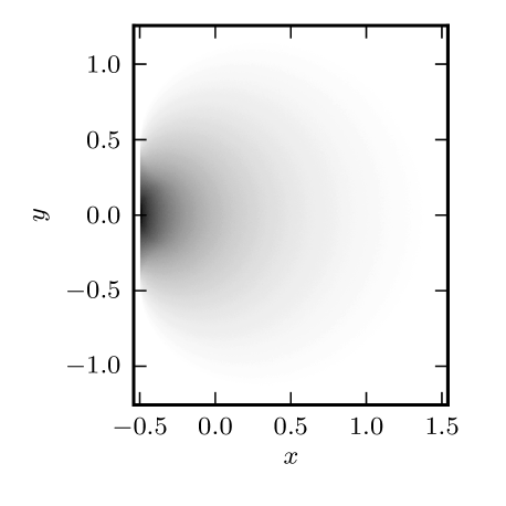
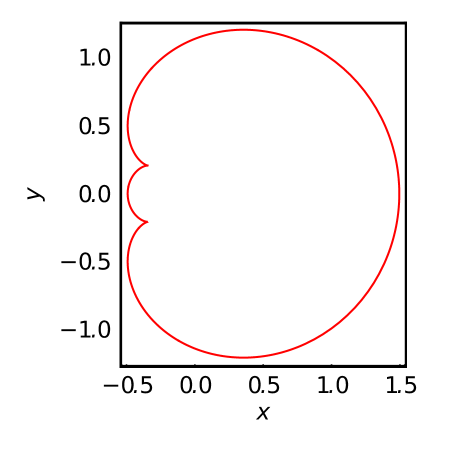
Figure 4: Numerical shadow for matrix $A_{2}$ of size $N=4$ and the corresponding critical lines.

The eigenvalues of $\mbox{Re}\left(e^{-i\theta}A_{2}\right)$ are $\frac{1}{2}\pm\cos\frac{\theta}{2},-\frac{1}{2}\pm\sin\frac{\theta}{2}$. The eigenvalues are $\left[\frac{3}{2},-\frac{1}{2},-\frac{1}{2},-\frac{1}{2}\right]$ at $\theta=0$ and $\pm\frac{1}{2}\pm\frac{\sqrt{2}}{2}$ at $\theta=\frac{\pi}{2}$. In the range $-\frac{\pi}{2}\leq\theta\leq\frac{\pi}{2}$ we have

$$\lambda_{4}\left(\theta\right)=\frac{1}{2}+\cos\frac{\theta}{2},\quad\lambda_{1}\left(\theta\right)=-\frac{1}{2}-\left|\sin\frac{\theta}{2}\right|,$$

and so $-\frac{1}{2}-\left|\sin\frac{\theta}{2}\right|\leq\mbox{Re}\left(e^{-i\theta}\psi^{*}A_{2}\psi\right)\leq\frac{1}{2}+\cos\frac{\theta}{2}$ for $\psi\in\Omega_{N}$. The triple eigenvalue $-\frac{1}{2}$ at $\theta=0$ results in a pronounced peak in the density for $\mbox{Re}(A_{2})$:

$$P_{2}(x)=6\left(\frac{1}{2}+x\right)_{+}\left(-x\right)_{+}^{2}+9\left(\frac{1}{2}+x\right)_{+}\left(-x\right)_{+}+\frac{27}{8}\left(\frac{1}{2}+x\right)_{+}^{2}\left(-x\right)_{+}^{0}$$

$$+\frac{3}{8}x_{+}^{0}\left(\frac{3}{2}-x\right)_{+}^{2}.$$

The matrix $A_{2}$ is non-generic and there is only one critical curve which has two cusps as shown in Fig. 4. In this example the boundary of the shadow is the convex hull of the critical curve, so the line segment $[(-1-i)/2,(-1+i)/2]$ is a part of the boundary. One representation of critical lines is $z=e^{i\theta}\left(\frac{1}{2}+\cos\frac{\theta}{2}-\frac{i}{2}\sin\frac{\theta}{2}\right),0\leq\theta\leq 4\pi$. The line segment joining $\frac{-1-i}{2}$ to $\frac{-1+i}{2}$ is part of the boundary of $\Lambda_{A_{2}}$. The cusps are at $\dfrac{-19\pm 5\sqrt{5}}{54}$.
Example 9.5.3 Let

$$A_{3}=\begin{pmatrix}0&1&1\\ 0&i&1\\ 0&0&-1\end{pmatrix}.$$

Then $m_{A_{3}}=\frac{1}{3}\left(-1+i\right)$,

$$\xi_{A_{3}}\left(s,t\right) = 1+\left(1-i\right)s+\left(1+i\right)t-i\left(s^{2}-t^{2}\right)-3st-st\left(\left(2-i\right)s+\left(2+i\right)t\right),$$

$$\xi_{A_{3}-m_{A_{3}}I}\left(s,t\right) = 1-\frac{13}{3}st-\frac{i}{3}\left(s^{2}-t^{2}\right)+\frac{5}{27}\left(\left(1+i\right)s^{3}+\left(1-i\right)t^{3}\right)$$

$$-\frac{st}{9}\left(\left(8+i\right)s+\left(8-i\right)t\right),$$

and

$$\xi_{\mbox{Re}\left(e^{-i\theta}A_{3}\right)}\left(r\right)=1+\left(\cos\theta-\sin\theta\right)r-\left(\frac{3}{4}+\sin\theta\cos\theta\right)r^{2}+\left(\frac{1}{4}\sin\theta-\frac{1}{2}\cos\theta\right)r^{3}.$$

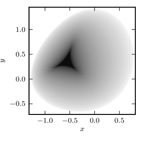
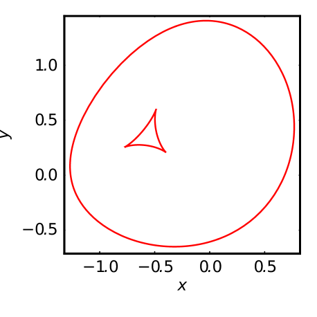
Figure 5: Numerical shadow for matrix $A_{3}$ of size $N=3$ and the corresponding critical lines.

The variance of $P_{\mbox{Re}\left(e^{-i\theta}A_{3}\right)}$ equals $\frac{1}{72}\left(13+2\sin 2\theta\right)$. The eigenvalues of $\mbox{Re}\left(e^{-i\theta}A_{3}\right)$ can be found approximately, or analytically by the classical formula. For $\theta=0$ the eigenvalues are $\left[-\frac{1+\sqrt{17}}{4},-\frac{1}{2},\frac{-1+\sqrt{17}}{4}\right]$ for $\theta=0$ and $\left[-0.6715,0.2647,1.407\right]$ (rounded) for $\theta=\frac{\pi}{2}$. The matrix is generic; there are two critical curves: one is the boundary of $\Lambda_{A_{3}}$ and the other is a triangular curve with three cusps. A comparison of the numerical shadow for this matrix and its critical lines is presented in Fig. 5. Since $N=3$ the density for $\mbox{Re}\left(e^{-i\theta}A_{3}\right)$ is piecewise linear:

$$P_{3}(x)=\left(-x\right)_{+}^{0}\left(x+\frac{1+\sqrt{17}}{4}\right)_{+}-2\left(-x\right)_{+}^{0}\left(x+\frac{1}{2}\right)_{+}$$

$$+\left(1-\frac{1}{\sqrt{17}}\right)x_{+}^{0}\left(\frac{\sqrt{17}-1}{4}-x\right)_{+}.$$

X Direct sums (block diagonal matrices)

Concerning the direct sum $A\oplus B$ (block diagonal matrix) of matrices $A,B$, it is well–known that

$$W(A\oplus B)={\mbox{conv}}\{W(A)\cup W(B)\}$$

(see, for example, [B1997, Exercise I.3.1]). In our context it is natural to ask how the numerical shadow of $A\oplus B$ is distributed over ${\mbox{conv}}\{W(A)\cup W(B)\}$. Here $A$ and $B$ may be of different sizes - see an example presented in Fig. 6. We consider then $A\oplus B\in M_{N}$ with $A\in M_{n}$ and $B\in M_{m}$, so that $n+m=N$. Given $u\in\Omega_{N}$ (distributed according to $\mu$, as usual), let $u=v_{1}\oplus v_{2}$ where $v_{1}\in{\mathbb{C}}^{n}$ and $v_{2}\in{\mathbb{C}}^{m}$; then $\|v_{1}\|^{2}+\|v_{2}\|^{2}=1$. It is known that $t=\|v_{1}\|^{2}$ has a beta–density given by

$$q(t)=\frac{(n+m-1)!}{(n-1)!\;(m-1)!}t^{n-1}(1-t)^{m-1}\quad(t\in[0,1]).$$ (38)

From this one can deduce that the shadow measure $P_{A\oplus B}$ is an “$(n,m)$–beta mixture” of the shadow measures $P_{A}$ and $P_{B}$. Compare [GS2010, section 2.2].

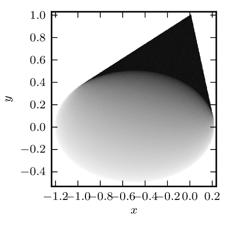
Figure 6: Shadow of block diagonal matrix $\left(\begin{smallmatrix}-1&0\\ 1&0\end{smallmatrix}\right)\oplus\left(\begin{smallmatrix}i\end{smallmatrix}\right)$ .

Another version of this result relates the densities corresponding to $A$, $B$, and $A\oplus B$:
Proposition 10.1: If $p_{A}(z),p_{B}(z)$ are the shadow densities for $A,B$, then the corresponding density $p$ for $A\oplus B$ is given by

$$p(z)=\int_{0}^{1}q(t)\Bigl{(}\int_{\mathbb{C}}t^{-2}p_{A}((z-w)/t)(1-t)^{-2}p_{B}\bigl{(}w/(1-t)\bigr{)}\,dw\Bigr{)}\,dt,$$ (39)

where $q(t)$ is as in (38).
Proof: For $u\in\Omega_{N}$ we have

$$\bigl{(}(A\oplus B)u,u\bigr{)}=(Av_{1},v_{1})+(Bv_{2},v_{2})$$

$$=\|v_{1}\|^{2}(Au_{1},u_{1})+\|v_{2}\|^{2}(Bu_{2},u_{2}),$$

where $u_{j}=v_{j}/\|v_{j}\|$. Note that $u_{1}\in\Omega_{n}$, $u_{2}\in\Omega_{m}$, $u_{1},u_{2}$ are stochastically independent, and they have the corresponding uniform distributions over $\Omega_{n}.\Omega_{m}$.
Hence $((A\oplus B)u,u)=tZ_{1}+(1-t)Z_{2}$ where $Z_{1}$ and $Z_{2}$ are independent complex random variables with densities $p_{A}(z)$ and $p_{B}(z)$. Thus

$$p(z)=\int_{0}^{1}q(t)g(z,t)\,dt$$

where $g(z,t)$ is the density of the independent (for each fixed $t$) sum $tZ_{1}+(1-t)Z_{2}$. This density is given by the usual convolution formula

$$g(z,t)=\int_{\mathbb{C}}g_{1}(z-w)g_{2}(w)\,dw,$$

where $g_{1}$ is the density of $tZ_{1}$ and $g_{2}$ is the density of $(1-t)Z_{2}$. If a complex random variable $Z$ has density $h(z)$ with respect to area on ${\mathbb{C}}$, then $tZ$ (where $t\in{\mathbb{R}}$) has density $t^{-2}h(z/t)$. Hence $g_{1}(z-w)=t^{-2}p_{A}((z-w)/t)$, $g_{2}(w)=(1-t)^{-2}p_{B}(w/(1-t))$ and (39) follows. QED

XI Zernike expansions

Given our methods for evaluating the moments of shadow measures (see section 5), it is natural to construct orthogonal polynomial approximations using Zernike polynomials. These provide one way to generate pictures of specific numerical shadows.
The complex Zernike polynomials $Z_{mn}\left(z,\overline{z}\right)$ are orthogonal for area measure on the unit disk $\left\{z\in\mathbb{C}:\left|z\right|\leq 1\right\}$. They can be defined by

$$Z_{mn}\left(z,\overline{z}\right)=z^{m-n}\sum_{j=0}^{n}\frac{\left(m+n-j\right)!}{\left(m-j\right)!\left(n-j\right)!j!}\left(-1\right)^{j}\left(z\overline{z}\right)^{n-j}\quad(m\geq n)$$

$$Z_{mn}\left(z,\overline{z}\right)=\overline{z}^{n-m}\sum_{j=0}^{m}\frac{\left(m+n-j\right)!}{\left(m-j\right)!\left(n-j\right)!j!}\left(-1\right)^{j}\left(z\overline{z}\right)^{n-j}\quad(m<n),$$

and satisfy the orthogonality relations

$$\frac{1}{\pi}\int\int_{\left|z\right|<1}Z_{mn}\left(z,\overline{z}\right)\overline{Z_{kl}\left(z,\overline{z}\right)}dm_{2}\left(z\right)=\frac{\delta_{mk}\delta_{nl}}{m+n+1}.$$

Suppose $f\left(z,\overline{z}\right)$ is continuous on the disk and has coefficients

$$\widehat{f}_{mn}:=\int\int_{\left|z\right|<1}f\left(z,\overline{z}\right)\overline{Z_{mn}\left(z,\overline{z}\right)}dm_{2}\left(z\right),m,n=0,1,2,\ldots$$

then

$$f=\frac{1}{\pi}\sum_{m=0}^{\infty}\sum_{n=0}^{\infty}\left(m+n+1\right)\widehat{f}_{mn}Z_{mn},$$

with convergence at least in the $L^{2}$-sense. As is typical of Fourier expansions, the convergence behaviour is better for smoother functions $f$. If $f$ is real then $\widehat{f}_{mn}=\overline{\widehat{f}_{nm}}$.
Suppose $A$ is an $N\times N$ matrix whose numerical range is contained in the unit disk (otherwise work with $B=c_{1}A+c_{0}I$, with $c_{1}>0$ so that ${\mbox{tr}}(B)=0$ and the range of $B$ satisfies the boundedness condition). We may use Proposition 5.3 to determine the moments of the shadow $P_{A}$ (and we write $dP_{A}\left(z\right)=p_{A}\left(z\right)dm_{2}\left(z\right)$, so that $p_{A}$ is the density). Thus

$$\int_{\left|z\right|\leq 1}z^{m}\overline{z}^{n}dP_{A}\left(z\right)=\frac{m!n!}{\left(N\right)_{m+n}}\left[s^{m}t^{n}\right]\xi_{A}\left(s,t\right)^{-1},$$

where $\xi_{A}\left(s,t\right)=\det\left(I-sA-tA^{*}\right)$ and $\left[s^{m}t^{n}\right]g\left(s,t\right)$ denotes the coefficient of $s^{m}t^{n}$ in the power series expansion of $g$ centered at $\left(s,t\right)=\left(0,0\right)$.
It is then straightforward to compute the Zernike coefficients of the density:

$$\left(p_{A}\right)_{mn}^{\char 94\relax} = \int_{\left|z\right|\leq 1}\overline{Z_{mn}\left(z,\overline{z}\right)}p_{A}\left(z\right)dm_{2}\left(z\right)$$

$$= \int_{\left|z\right|\leq 1}\sum_{j=0}^{n}\frac{\left(m+n-j\right)!}{\left(m-j\right)!\left(n-j\right)!j!}\left(-1\right)^{j}z^{n-j}\overline{z}^{m-j}dP_{A}\left(z\right)$$

$$= \sum_{j=0}^{n}\frac{\left(m+n-j\right)!}{j!\left(N\right)_{m+n-2j}}\left(-1\right)^{j}\left[s^{n-j}t^{m-j}\right]\xi_{A}\left(s,t\right)^{-1},$$

for $m\geq n$ (and $\left(p_{A}\right)_{nm}^{\char 94\relax}=\overline{\left(p_{A}\right)_{mn}^{\char 94\relax}}$ ). As an approximation, one may compute $\left(p_{A}\right)_{mn}^{\char 94\relax}$ for all $\left(m,n\right)$ with $m+n\leq M$ for some $M$ (say 10 or 20). To write our formulas in real terms with $z=x+iy$ (and $x^{2}+y^{2}\leq 1$), let

$$Q_{mn}\left(u\right)=\sum_{j=0}^{\min\left(m,n\right)}\frac{\left(m+n-j\right)!}{\left(m-j\right)!\left(n-j\right)!j!}\left(-1\right)^{j}u^{\min\left(m,n\right)-j}.$$

Note the trivial identity $ab+\overline{a}\overline{b}=2\mbox{Re}a\mbox{Re}b-2\mbox{Im}a\mbox{Im}b$. Thus the partial sum for $p_{A}$ can be written as:

$$\sum_{j=0}^{\left\lfloor M/2\right\rfloor}\left(2j+1\right)\left(p_{A}\right)_{jj}^{\char 94\relax}Q_{jj}\left(x^{2}+y^{2}\right)+$$

$$+2\sum_{j=1}^{M}\left(\mbox{Re}\left(\left(x+\mathrm{i}y\right)^{j}\right)\sum_{n=0}^{\left\lfloor\left(M-j\right)/2\right\rfloor}\left(2n+j+1\right)\mbox{Re}\left(\left(p_{A}\right)_{n+j,n}^{\char 94\relax}\right)Q_{n+j,n}\left(x^{2}+y^{2}\right)\right)$$

$$-2\sum_{j=1}^{M}\left(\mbox{Im}\left(\left(x+\mathrm{i}y\right)^{j}\right)\sum_{n=0}^{\left\lfloor\left(M-j\right)/2\right\rfloor}\left(2n+j+1\right)\mbox{Im}\left(\left(p_{A}\right)_{n+j,n}^{\char 94\relax}\right)Q_{n+j,n}\left(x^{2}+y^{2}\right)\right).$$

(The factor $\pi$ has been ignored; it is merely a change of scale). It is a matter for experimentation to produce useful graphs for a given matrix. The polynomials tend to wiggle close to the edge of the disk; the graphs can not be expected to precisely show the boundary of the numerical range, but they do indicate the behaviour of $p_{A}$ in the interior.

XII Numerical shadows and the higher–rank numerical ranges

The rank–$k$ numerical ranges, denoted below by $\Lambda_{k}$, were introduced c. 2006 by Choi, Kribs, and Życzkowski as a tool to handle compression problems in quantum information theory. Since then their theory and applications have been advanced with remarkable enthusiasm. The sequence of papers [CHKŻ2007,CGHK2008,W2008,LS2008], for example, led to a striking extension of the classical Toeplitz–Hausdorff theorem (convexity of $W(M)$): all the $\Lambda_{k}(M)$ are convex (though some may be empty), and they are intersections of conveniently computable half–planes in ${\mathbb{C}}$. Among the many more recent papers concerning the $\Lambda_{k}(M)$, let us mention [LPS2009,GLW2010].
Given a matrix $M\in M_{N}$ and $k\geq 1$, Choi, Kribs, and Życzkowski (see [CKŻ2006a,CKŻ2006b]) defined the rank–$k$ numerical range of $M$ as

$$\Lambda_{k}(M)=\{{\lambda}\in{\mathbb{C}}:\exists P\in P_{k}\mbox{ such that }PMP={\lambda}P\},$$

where $P_{k}$ denotes the set of rank–$k$ orthogonal projections in $M_{N}$. It is not hard to verify that $\Lambda_{K}(M)$ can also be described as the set of complex ${\lambda}$ such that there is some $k$–dimensional subspace $S$ of ${\mathbb{C}}^{N}$ such that $(Mu,u)={\lambda}$ for all unit vectors in $S$. In particular, we see that

$$W(M)=\Lambda_{1}(M)\supseteq\Lambda_{2}(M)\supseteq\Lambda_{3}(M)\supseteq\dots\quad.$$

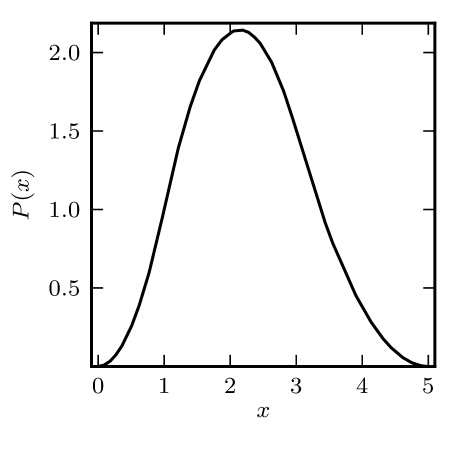
(a)

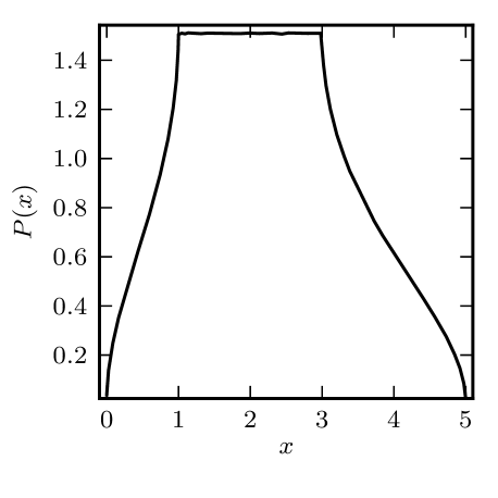
(b)

Figure 7:

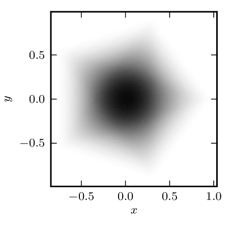
(a)

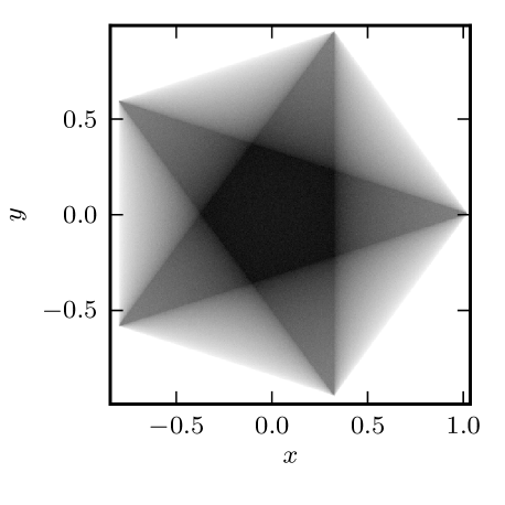
(b)

Figure 8:

This point of view also suggests that these higher–rank numerical ranges should be visible as regions of higher density within the numerical shadow of $M$. This idea is borne out, to some degree, by examining shadow densities of various matrices. In Figure 7(a), for example, we see the (one–dimensional) shadow density of the Hermitian ${\mbox{diag}}(0,1,3,5)$ - a spline of degree 2. Here it is known that $\Lambda_{2}(M)=[1,3]$; while the density is unimodal, there are values in [3,5] that are greater than some in [1,3]. If real unit vectors are used in such experiments, the higher–rank numerical ranges often seem to be revealed more clearly.; compare Figure 7(b).

A similar phenomenon is seen in Figure 8. Here $M$ is a unitary matrix in $M_{5}$ and it is known that $\Lambda_{2}(M)$ is the inner pentagon (with interior) formed by lines joining the non–adjacent eigenvalues in pairs. The shadow density is unimodal, but $\Lambda_{2}(M)$ is only seen distinctly in Figure 8(b), where only real unit vectors in $u\in\Omega_{5}$ are use to generate the values $(Mu,u)$. The distinction between shadows based on complex vs real unit vectors is a reflection of the fact that the latter follow a Dirichlet distribution (with parameter 1/2) rather than our usual measure $\mu$. See [BŻ2006].

References

- A (1971) T. W. Anderson, The Statistical Analysis of Time Series, Wiley, New York, 1971.
- B (1997) R. Bhatia, Matrix Analysis, Springer–Verlag, New York, 1997.
- BŻ (2006) I. Bengtsson and K. Życzkowski, Geometry of Quantum States, Cambridge UP, Cambridge, 2006.
- CK (1985) E. W. Cheney and D. R. Kincaid, Numerical Mathematics and Computing, Brooks/Cole 1985.
- (5) M.–D. Choi, D. Kribs, and K. Życzkowski, Quantum error correcting codes from the compression formalism, Rep. Math. Phys. 58 (2006) 77–86.
- (6) M.–D. Choi, D. Kribs, and K. Życzkowski, Higher–rank numerical ranges and compression problems, Linear Alg. Appl. 418 (2006) 828–839.
- CHKŻ (2007) M.–D. Choi, J. Holbrook, D. Kribs, and K. Życzkowski, Higher–rank numerical ranges of unitary and normal matrices, Operators and Matrices 1 (2007) 409–426.
- CGHK (2008) M.–D. Choi, M. Giesinger, J. Holbrook, and D. Kribs, Geometry of higher–rank numerical ranges, Linear and Multilinear Algebra 56 (2008) 53-64.
- DH (1988) K. R. Davidson and J. Holbrook, Numerical radii of zero-one matrices, Michigan Math. J. 35 (1988) 261–267.
- DJ (2007) D. Ž. Djoković and C. R. Johnson, Unitarily achievable zero patterns and traces of words in and , Linear Alg. Appl. 421 (2007) 63–68.
- D (1971) C. Davis, The Toeplitz–Hausdorff theorem explained, Canad. Math. Bull. 14 (1971) 245–246.
- dB (1976) C. de Boor, Splines as linear combinations of B-splines, pp. 1-47 in Approximation Theory II (G.G. Lorentz, C. K. Chui, and L. L. Schumaker, eds.), Academic Press, New York, 1976.
- GLW (2010) H.–L. Gau, C.–K. Li, and P. Y. Wu, Higher –rank numerical ranges and dilations, J. Operator Theory 63 (2010) 181-189.
- GR (1997) K. E. Gustafson and D. K. M. Rao, Numerical Range, Springer, 1997.
- GS (2010) T. Gallay and D. Serre, The numerical measure of a complex matrix, arXiv:1009.1522v1 [math.FA], 8Sep2010
- He (1984) S. Helgason, Groups and Geometric Analysis, Academic Press, New York, 1984.
- Hn (1974) P. Henrici, Applied and Complex Analysis, Vol. 1, Wiley-Interscience, New York 1974.
- H (2010) J. Holbrook, Diagonal compressions of matrices and numerical shadows, colloquium, Feb 19, U. of Hawaii, 2010
- HS (2010) J. Holbrook and J.–P. Schoch, Theory vs. experiment: multiplicative inequalities for the numerical radius of commuting matrices, Operator Theory: Advances and Applications 202 (2010) 273–284.
- JAG (1998) E. Jonckheere, F. Ahmad, and E. Gutkin, Differential topology of numerical range, Linear Alg. Appl. 279 (1998) 227–254.
- L (2001) C.–K. Li, A survey on linear preservers of numerical ranges and radii, Taiwanese J. Math. 5 (2001) 477–496.
- LPS (2009) C.–K. Li, Y.–T. Poon, and N.–S. Sze, Condition for the higher–rank numerical range to be non–empty, Linear and Multilinear Algebra 57 (2009) 365–368.
- LS (2008) C.–K. Li and N.–S. Sze, Canonical forms, higher rank numerical ranges, totally isotropic subspaces, and matrix equations, Proc. Amer. Math. Soc. 136 (2008) 3013–3023.
- Mac (1995) I. G. Macdonald, Symmetric Functions and Hall Polynomials, II ed., Clarendon Press, Oxford, 1995.
- N (1982) K.–C. Ng, Some properties of doubly-stochastic matrices and distribution of density on a numerical range, MPhil thesis, U of Hong Kong, 1982
- S (1940) W. Specht, Zur Theorie der Matrixen II, Jahresber. Deutsche Math. 50 (1940) 19–23.
- W (2008) H. Woerdeman, The higher rank numerical range is convex, Linear and Multilinear Algebra 56 (2008) 65–67.
- Ż (1999) K. Życzkowski, Volume of the set of separable states II, Phys. Rev. A60 (1999) 3496–3507.
- Ż (2009) K. Życzkowski (with M.–D. Choi, C. Dunkl, J. Holbrook, P. Gawron, J.Miszczak, Z. Puchala, and L. Skowronek), Generalized numerical range as a versatile tool to study quantum entanglement, Oberwolfach, Dec 2009 (see Oberwolfach Report No. 59/2009, 34–37), 2009