Unitary and causal dynamics based
on the chiral Lagrangian

Abstract

Pion-nucleon scattering, pion photoproduction, and nucleon Compton scattering are analyzed within a scheme based on the chiral Lagrangian. Partial-wave amplitudes are obtained by an analytic extrapolation of subthreshold reaction amplitudes computed in chiral perturbation theory, where the constraints set by electromagnetic-gauge invariance, causality and unitarity are used to stabilize the extrapolation. Experimental data are reproduced up to energies $\sqrt{s}\simeq 1300$ MeV in terms of the parameters relevant at order $Q^{3}$. A striking puzzle caused by an old photon asymmetry measurement close to the pion production threshold is discussed.

1 Introduction

In recent years photon- and pion-nucleon interactions have been successfully used as a quantitative challenge of chiral perturbation theory ($\chi$PT), which is a systematic tool to learn about low-energy QCD dynamics Bernard et al. (1995); Bernard (2008); Pascalutsa et al. (2007). The application of $\chi$PT is limited to the near threshold region. The pion-nucleon phase shifts have been analyzed in great depth at subleading orders in the chiral expansion Bernard et al. (1997); Fettes et al. (1998); Fettes and Meissner (2000). Pion photoproduction was studied in Bernard et al. (1992, 1996a, 1996b); Fearing et al. (2000). Compton scattering was considered in Bernard et al. (1995); Beane et al. (2005).

The purpose of this talk is to report on a novel and unified description of photon and pion scattering off the nucleon based on the chiral Lagrangian Gasparyan and Lutz (2010). We aim at a description from threshold up to and beyond the isobar region in terms of partial-wave amplitudes that are consistent with the constraints set by causality and unitarity. Our analysis is based on the chiral Lagrangian with pion and nucleon fields truncated at order $Q^{3}$. We do not consider an explicit isobar field in the chiral Lagrangian. The physics of the isobar resonance enters our scheme by an infinite summation of higher order counter terms in the chiral Lagrangian. The particular summation is performed in accordance with unitarity and causality.

The scheme is based on an analytic extrapolation of subthreshold scattering amplitudes that is controlled by constraints set by electromagnetic-gauge invariance, causality and unitarity. Unitarized scattering amplitudes are obtained which have left-hand cut structures in accordance with causality. The latter are solutions of non-linear integral equations that are solved by $N/D$ techniques. The integral equations are imposed on partial-wave amplitudes that are free of kinematical zeros and singularities. An essential ingredient of the scheme is the analytic continuation of the generalized potentials that determine the partial-wave amplitudes via the non-linear integral equation. We discuss the analytic structure of the generalized potentials in detail and construct suitable conformal mappings in terms of which the analytic continuation is performed systematically. Contributions from far distant left-hand cut structures are represented by power series in the conformal variables.

The relevant counter terms of the Lagrangian are adjusted to the empirical data available for photon and pion scattering off the nucleon. We focus on the s- and p-wave partial-wave amplitudes and do not consider inelastic channels with two or more pions. We recover the empirical s- and p-wave pion-nucleon phase shifts up to about 1300 MeV quantitatively. The pion photoproduction process is analyzed in terms of its multipole decomposition. Given the significant ambiguities in those multipoles we offer a more direct comparison of our results with differential cross sections and polarization data. A quantitative reproduction of the data set up to energies of about $\sqrt{s}\simeq 1300$ MeV is achieved.

2 Analytic extrapolation of subthreshold scattering amplitudes

The starting point of our method is the chiral Lagrangian involving pion, nucleon and photon fields Fettes et al. (1998); Bernard (2008), for which we collect the relevant terms

$$\mathcal{L}_{int} = -\frac{1}{4\,f^{2}}\,\bar{N}\,\gamma^{\mu}\,\big{(}\vec{\tau}\cdot\big{(}\vec{\pi}\times(\partial_{\mu}\vec{\pi})\big{)}\big{)}\,N+\frac{g_{A}}{2\,f}\,\bar{N}\,\gamma_{5}\,\gamma^{\mu}\,\big{(}\vec{\tau}\cdot(\partial_{\mu}\vec{\pi})\big{)}\,N$$ (1)

$$- e\,\Big{\{}\big{(}\vec{\pi}\times(\partial_{\mu}\vec{\pi})\big{)}_{3}+\bar{N}\,\gamma_{\mu}\,\frac{1+\tau_{3}}{2}\,N-\frac{g_{A}}{2\,f}\,\bar{N}\,\gamma_{5}\,\gamma_{\mu}\,\big{(}\vec{\tau}\times\vec{\pi}\big{)}_{3}\,N\Big{\}}\,A^{\mu}$$

$$- \frac{e}{4\,m_{N}}\,\bar{N}\,\sigma_{\mu\nu}\,\frac{\kappa_{s}+\kappa_{v}\,\tau_{3}}{2}\,N\,F^{\mu\nu}+\frac{e^{2}}{32\pi^{2}f}\,\epsilon^{\mu\nu\alpha\beta}\,\pi_{3}\,F_{\mu\nu}\,F_{\alpha\beta}$$

$$- \frac{2\,c_{1}}{f^{2}}\,m_{\pi}^{2}\,\bar{N}\,(\vec{\pi}\cdot\vec{\pi})\,N-\frac{c_{2}}{2\,f^{2}\,m_{N}^{2}}\,\Big{\{}\bar{N}\,(\partial_{\mu}\,\vec{\pi})\cdot(\partial_{\nu}\vec{\pi})\,(\partial^{\mu}\partial^{\nu}N)+\rm{h.c.}\Big{\}}$$

$$+ \frac{c_{3}}{f^{2}}\,\bar{N}\,(\partial_{\mu}\,\vec{\pi})\cdot(\partial^{\mu}\vec{\pi})\,N-\frac{c_{4}}{2\,f^{2}}\,\bar{N}\,\sigma^{\mu\nu}\,\big{(}\vec{\tau}\cdot\big{(}(\partial_{\mu}\vec{\pi})\times(\partial_{\nu}\vec{\pi})\big{)}\big{)}\,N$$

$$- i\,\frac{d_{1}+d_{2}}{f^{2}\,m_{N}}\,\bar{N}\,\big{(}\vec{\tau}\cdot\big{(}(\partial_{\mu}\vec{\pi})\times(\partial_{\nu}\partial_{\mu}\vec{\pi})\big{)}\big{)}\,(\partial^{\nu}N)+\rm{h.c.}$$

$$+ \frac{i\,d_{3}}{f^{2}\,m_{N}^{3}}\,\bar{N}\,\big{(}\vec{\tau}\cdot\big{(}(\partial_{\mu}\vec{\pi})\times(\partial_{\nu}\partial_{\lambda}\vec{\pi})\big{)}\big{)}\,(\partial^{\nu}\partial^{\mu}\partial^{\lambda}N)+\mbox{h.c.}$$

$$- 2\,i\,\frac{m_{\pi}^{2}\,d_{5}}{f^{2}\,m_{N}}\,\bar{N}\,\big{(}\vec{\tau}\cdot\big{(}\vec{\pi}\times(\partial_{\mu}\vec{\pi})\big{)}\big{)}\,(\partial^{\mu}N)+\rm{h.c.}$$

$$- \frac{i\,e}{f\,m_{N}}\,\epsilon^{\mu\nu\alpha\beta}\,\bar{N}\,\big{(}d_{8}\,(\partial_{\alpha}\,\pi_{3})+d_{9}\,\big{(}\vec{\tau}\cdot(\partial_{\alpha}\vec{\pi})\big{)}\big{)}\,(\partial_{\beta}\,N)\,F_{\mu\nu}+\mbox{h.c.}$$

$$+ i\,\frac{d_{14}-d_{15}}{2\,f^{2}\,m_{N}}\,\bar{N}\,\sigma^{\mu\nu}\,\big{(}(\partial_{\nu}\vec{\pi})\cdot(\partial_{\mu}\partial_{\lambda}\vec{\pi})\big{)}\,(\partial^{\lambda}N)+\mbox{h.c.}$$

$$- \frac{m_{\pi}^{2}\,d_{18}}{f}\,\bar{N}\,\gamma_{5}\,\gamma^{\mu}\,\big{(}\vec{\tau}\cdot(\partial_{\mu}\vec{\pi})\big{)}\,N$$

$$+ \frac{e\,(d_{22}-2\,d_{21})}{2\,f}\,\bar{N}\,\gamma_{5}\,\gamma^{\mu}\,\big{(}\vec{\tau}\times\partial^{\nu}\,\vec{\pi}\big{)}_{3}\,N\,F_{\mu\nu}$$

$$+ \frac{e\,d_{20}}{2\,f\,m_{N}^{2}}\,\bar{N}\,\gamma_{5}\,\gamma^{\mu}\,\big{(}\vec{\tau}\times(\partial_{\lambda}\,\vec{\pi})\big{)}_{3}\,(\partial^{\nu}\partial^{\lambda}N)\,F_{\mu\nu}+\mbox{h.c.}\,.$$

In a strict chiral expansion the order $Q^{3}$ results are composed from a tree-level part and a one-loop part. Both parts are invariant under electromagnetic gauge transformations separately. The tree-level pion-nucleon scattering amplitude receives contributions from the Weinberg-Tomozawa term, the s- and u-channel nucleon exchange processes and the $Q^{2}$ and $Q^{3}$ counter terms characterized by the parameters $c_{1},...,c_{4}$ and $d_{1}+d_{2},d_{3},d_{5},d_{14}-d_{15},d_{18}$. At tree-level the pion photoproduction amplitude is determined by the Kroll-Rudermann term, the nucleon s- and u-channel exchange processes and the t-channel pion exchange. At chiral order $Q^{3}$ the counter terms $d_{8},d_{9},d_{18},2\,d_{21}-d_{22}$ contribute. The tree-level amplitude for the proton Compton scattering is given by nucleon s- and u-channel exchange contribution and pion t-channel exchange.

Our approach is based on partial-wave dispersion relations, for which the unitarity and causality constraints can be combined in an efficient manner. Using a partial-wave decomposition simplifies calculations because of angular momentum and parity conservation. For a suitably chosen partial-wave amplitude with angular momentum $J$, parity $P$ and channel quantum numbers $a,b$ we separate the right-hand cuts from the left-hand cuts

$$T_{ab}^{(JP)}(\sqrt{s}\,)=U_{ab}^{(JP)}(\sqrt{s}\,)+\int_{\mu_{\rm thr}}^{\infty}\frac{dw}{\pi}\frac{\sqrt{s}-\mu_{M}}{w-\mu_{M}}\frac{\Delta T_{ab}^{(JP)}(w)}{w-\sqrt{s}-i\epsilon}\,,$$ (2)

where the generalized potential, $U_{ab}^{(JP)}(\sqrt{s}\,)$, contains left-hand cuts only, by definition. The separation (2) is gauge invariant. This follows since both contributions in (2) are strictly on-shell and characterized by distinct analytic properties. The amplitude is considered as a function of $\sqrt{s}$ due to the MacDowell relations MacDowell (1959). A subtraction is made at $\sqrt{s}=\mu_{M}=m_{N}$ for the reasons to be discussed below.

The condition that the scattering amplitude must be unitary allows one to calculate the discontinuity along the right-hand cut

$$\Delta T_{ab}^{(JP)}(\sqrt{s}) = \frac{1}{2\,i}\left(T_{ab}^{(JP)}(\sqrt{s}+i\epsilon)-T_{ab}^{(JP)}(\sqrt{s}-i\epsilon)\right)$$ (3)

$$= \sum_{c,d}\,T_{ac}^{(JP)}(\sqrt{s}+i\epsilon)\,\rho^{(JP)}_{cd}(\sqrt{s}\,)\,T_{db}^{(JP)}(\sqrt{s}-i\epsilon),$$

where, $\rho^{(JP)}_{cd}(\sqrt{s}\,)$, is the phase-space matrix. The relation (2) illustrates that the amplitude possesses a unitarity cut along the positive real axis starting from the lowest $s$-channel threshold. In our case the $\gamma\,N$ intermediate states induce a branch point at $\sqrt{s}=\mu_{\rm thr}=m_{N}$, which defines the lowest s-channel unitarity threshold.

The structure of the left-hand cuts in $U_{ab}^{(JP)}(\sqrt{s}\,)$ can be obtained by assuming the Mandelstam representation Mandelstam (1958); Ball (1961) or examining the structure of Feynman diagrams in perturbation theory Nakanishi (1962). At leading order one may try to identify the generalized potential, $U_{ab}(\sqrt{s}\,)$, with a partial-wave projected tree-level amplitude. After all the tree-level expressions do not show any right-hand unitarity cuts. However, this is an ill-defined strategy since it would lead to an unbounded generalized potential for which the non-linear system (2, 3) does not allow any solution.

The key observation is the fact that the solution of (2, 3) requires the knowledge of the generalized potential for $\sqrt{s}>\mu_{\rm thr}$ only. Conformal mapping techniques Frazer (1961) may be used to approximate the generalized potential in that domain efficiently based on the knowledge of the generalized potential in a small subthreshold region around some expansion point $\mu_{E}$ only, where it may be computed reliably in $\chi$PT. We establish a representation of the generalized potential of the form

$$U(\sqrt{s}\,)=U_{\rm inside}(\sqrt{s}\,)+U_{\rm outside}(\sqrt{s}\,)\,,$$ (4)

$$U_{\rm outside}(\sqrt{s}\,)=\sum\limits_{k=0}^{\infty}{U_{k}}\,\big{[}\xi(\sqrt{s}\,)\big{]}^{k}\,,\qquad U_{k}=\frac{d^{k}U_{\rm outside}(\xi^{-1}(\xi))}{k!\,d\xi^{k}}\Big{|}_{\xi=0}\,,$$

where we allow for an explicit treatment of left-hand cut structures that are inside a given domain $\Omega$. The conformal mapping $\xi(\sqrt{s}\,)$ is defined unambiguously with

$$\xi(\mu_{E}\,)=0\,,$$ (5)

and by the region $\Omega$, in which the expansion of $U_{\rm outside}(\sqrt{s}\,)$ is converging. The region $\Omega$ includes the real interval $(\mu_{E},\Lambda)$ where the parameter $\Lambda<\infty$ locates the opening of further inelastic channels not considered explicitly. For $\sqrt{s}>\Lambda$ the outside part of the potential is set to a constant for convenience, where a suitable construction of the conformal mapping leads to a continuous behavior of $U_{\rm outside}(\sqrt{s}\,)$ and $U^{\prime}_{\rm outside}(\sqrt{s}\,)$ at $\sqrt{s}=\Lambda$. It is important to realize that the generalized potential is a smooth and analytic function for $\mu_{E}<\sqrt{s}<\Lambda$.

For the elastic $\pi N\to\pi N$ potential the presence of baryon resonances is encoded in the behavior of the potential at $\sqrt{s}<m_{N}-m_{\pi}$, a region not required to solve the non-linear system (2, 3). While at the matching scale $\sqrt{s}\simeq\mu_{M}$ we assume a perturbative behavior of the generalized potential, this is no longer justified as the energy $\sqrt{s}$ is decreasing down to the region characterized by the u-channel exchange of baryon resonances. Thus it is natural to insist on that the domain $\Omega$, excludes the u-channel unitarity branch cuts. Such a construction lives in harmony with the crossing symmetry of the scattering amplitude. Given the assumption the generalized potential cannot be evaluated by means of the representation (4) for $\sqrt{s}<m_{N}-m_{\pi}$. The decomposition (4) is faithful for energies $\sqrt{s}\in\Omega$ only. Nevertheless, the full scattering amplitude can be reconstructed at $\sqrt{s}\leq m_{N}-m_{\pi}$ from the knowledge of the generalized potential at $\sqrt{s}>m_{N}+m_{\pi}$ by a crossing transformation of the solution to (2, 3). Such a construction is consistent with crossing symmetry if the solution to (2, 3) and its crossing transformed form coincide in the region $m_{N}-m_{\pi}<\sqrt{s}<m_{N}+m_{\pi}$. This is the case approximatively, if the matching scale $\mu_{M}$ in (2) is identified properly. For $m_{N}-m_{\pi}<\mu_{M}<m_{N}+m_{\pi}$ the scattering amplitude remains perturbative in the matching interval, at least sufficiently close to $\sqrt{s}\sim\mu_{M}$. With our choice

$$\mu_{M}=m_{N}\,,$$ (6)

this is clearly the case (see also Lutz and Kolomeitsev (2002)).

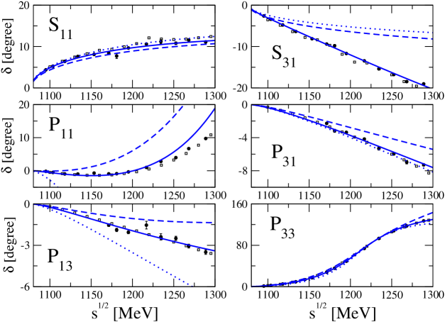
Figure 1: Results of the fit for $\pi N$ $S$ and $P$-wave phase shifts. The solid curves correspond to the full $Q^{3}$ results, the dashed curves to $Q^{2}$ results, and the dotted curves to $Q^{1}$ calculation. The data are from Koch (1986)(circles) and Arndt et al. (2006)(squares).

3 Results

We performed numerical calculations for the three reactions $\pi N\to\pi N$, $\gamma N\to\pi N$ and $\gamma N\to\gamma N$, where we assume the $\pi N$ channel in an s- or p-wave state Gasparyan and Lutz (2010). The considered energy region from threshold up to $1.3$ GeV is motivated by the expected reliability of the two-channel approximation Koch (1986); Arndt et al. (2006). The $\pi N$ sector is developed independently from the $\gamma N$ channel as it is treated to first order in the electric charge. After adjustment of the free parameters we obtain a good description of the empirical phase shifts. There are four $Q^{2}$ counter terms $c_{1-4}$. Further four parameters $d_{1}+d_{2}$, $d_{3,5}$ and $d_{14-15}$ are relevant at the one-loop level $Q^{3}$. As can be seen from Fig. 1 for all partial waves we obtain a convincing convergence pattern. For a more detailed discussion, in particular the presence of CDD poles in the $P_{11}$ and $P_{33}$ waves we refer to Gasparyan and Lutz (2010).

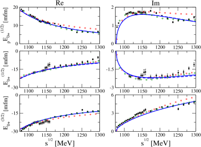
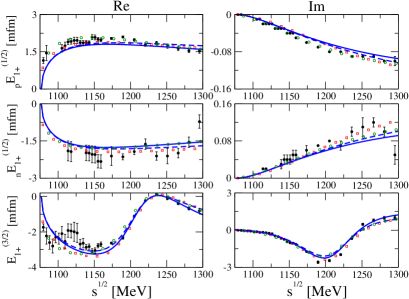
Figure 2: Electric photoproduction multipoles $E_{0+}$ and $E_{1+}$. The data are from Arndt et al. (2002)(filled circles – energy independent analyses, open circles – energy dependent analysis) and Drechsel et al. (2007)(squares). The solid line denotes the $Q^{3}$ calculation, the dashed line – $Q^{2}$ calculation.

We turn to pion photoproduction, which requires the determination of additional parameters. Besides further parameters describing the coupling of the CDD poles to the $\gamma N$ channel there are additional counter terms of the chiral Lagrangian to be considered. The relevant parameter set is obtained in part from the empirical s- and p-wave multipoles. There are significant discrepancies among different energy-dependent analyses Arndt et al. (2002); Drechsel et al. (2007). Therefore we use the energy independent partial-wave analysis from Arndt et al. (2002), which is less biased than the energy dependent multipole analyses. Since the imaginary parts of the multipoles are given by Watson’s theorem Watson (1954), their real parts are considered only. We find the $\pi N$ rescattering effects important for the real parts of the s-wave multipoles. For the $p$-wave multipoles, which do not have a CDD pole contribution, rescattering effects are mostly responsible for generating the correct imaginary part, but do not modify the real parts much. The s-wave multipoles shown in Fig. 2 depend on the particular counter term combination

$$\bar{d}_{20}+\frac{2\,\bar{d}_{21}-\bar{d}_{22}}{2}\,.$$ (7)

Since none of the other multipoles depend on $\bar{d}_{20}$, the parameter combination (7) is determined by the empirical s-wave multipoles. Given the spread in the different energy dependent analyses a satisfactory description of the s-wave multipoles is obtained.

The magnetic multipole $M_{1+}^{(3/2)}$ multipole provides a large and dominant contribution to the cross sections in the $\Delta(1232)$ resonance region Arndt et al. (2002); Drechsel et al. (2007). As a consequence the empirical error bars for this multipole are very small. The multipole depends on the particular parameter combination

$$\bar{d}_{8}+\frac{2\,\bar{d}_{21}-\bar{d}_{22}}{2}\,,$$ (8)

which is relevant also for the electric multipole $E_{1+}^{(3/2)}$. The solid lines in Fig. 2 and Fig. 3 show that a satisfactory description for both multipoles is obtained.

There remain two parameter combinations, $\bar{d}_{9}$ and $2\,\bar{d}_{21}-\bar{d}_{22}$, that cannot be determined unambiguously from the energy independent multipole analysis Arndt et al. (2002). Incidentally, the energy dependent analyses Arndt et al. (2002); Drechsel et al. (2007) differ most significantly in the remaining five magnetic multipoles of Fig.  3, which are sensitive to the latter parameters. The determination of our preferred values took into account additional constraints from photoproduction cross sections and Compton scattering data. The resulting five magnetic multipoles are shown in Fig. 3.

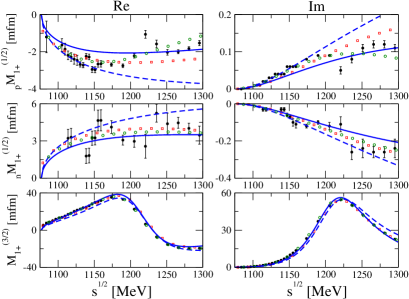
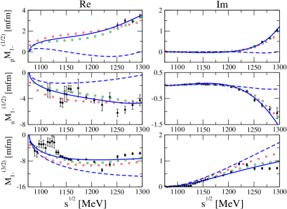
Figure 3: Magnetic photoproduction multipoles $M_{1+}$ and $M_{1-}$. The data and line conventions are as in Fig. 2.

Empirically it is well established that in neutral pion photoproduction there is a strong cusp effect at the $\pi^{+}\,n$ threshold Bergstrom et al. (1996); Schmidt et al. (2001). To obtain accurate results we depart from the isospin formulation and perform a coupled-channel computation in the particle basis using physical masses for the nucleons and pions. Isospin breaking effects are not considered for the generalized potential being estimated to be of minor importance. No additional parameters arise. Since the threshold region shows an intriguing interplay of the s- and p-wave multipoles we confront our theory in Fig. 4 with empirical differential cross section of the Mainz group directly. Given the fact that we did not fit the parameters to those data an excellent description is achieved.

To further scrutinize the threshold region it is customary to introduce the following three combinations of p-wave multipole amplitudes,

$$\bar{p}_{\rm cm}\,\bar{P}_{1}=3\,E_{1+}+M_{1+}-M_{1-}\,,\qquad\bar{p}_{\rm cm}\,\bar{P}_{2}=3\,E_{1+}-M_{1+}+M_{1-}\,,$$

$$\bar{p}_{\rm cm}\,\bar{P}_{3}=2\,M_{1+}+M_{1-}\,,$$ (9)

which all vanish at the production threshold with $\bar{p}_{\rm cm}=0$. At leading orders in a chiral expansion $\bar{P}_{1}$ and $\bar{P}_{2}$ do not depend on any of the $Q^{3}$ counter terms. The threshold behavior of $\bar{P}_{1}$ and $\bar{P}_{2}$ is predicted in terms of the electromagnetic charge, the pion-nucleon coupling constant and the masses of the pions and nucleons only Bernard et al. (1996a, c, 2001). In contrast $\bar{P}_{3}$ receives a contribution from the $Q^{3}$ counter term combination $\bar{d}_{8}+\bar{d}_{9}$ and there is no parameter-free prediction accurate to order $Q^{3}$. Since in our analysis all counter terms have been adjusted to photo-production data excluding the near threshold region we can predict the threshold values of the three amplitude $\bar{P}_{1-3}$. We observe a striking disagreement with the values obtained in Schmidt et al. (2001).

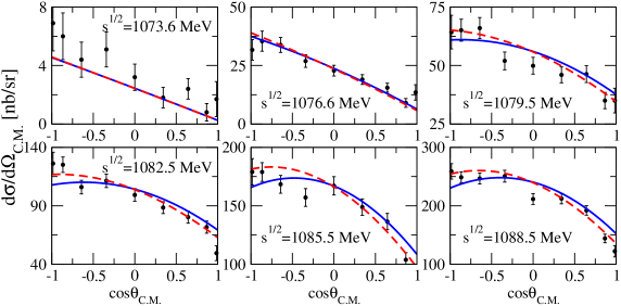
Figure 4: Near threshold differential cross section for the reaction $\gamma p\to\pi^{0}p$ with data taken from Schmidt (2001); Schmidt et al. (2001). Shown are results from our coupled-channel theory including isospin breaking effects as are implied by the use of empirical pion and nucleon masses. The solid lines correspond to our calculation with only $s$- and $p$-wave multipoles included. The effect of higher partial waves is shown by the dashed lines.

From the near-threshold differential cross section two combinations of p-wave threshold parameters may be extracted. A complete determination of all three threshold amplitudes requires additional information. For this purpose a measurement of the near-threshold photon asymmetry suffices Schmidt et al. (2001). A direct comparison with the near-threshold photon asymmetry measurement of the Mainz group Schmidt et al. (2001) is not straightforward since an average from threshold to 166 MeV laboratory photon energies was performed. In Fig. 5 we show the result of our computation at four different energies demonstrating a sign change in the asymmetry at energies below the mean value of 159.5 MeV in the Mainz experiment. At the mean energy our photon asymmetry is about a factor four to five smaller than the averaged value presented in Schmidt et al. (2001). A significant effect of higher partial wave contributions on the asymmetry is illustrated by the dashed lines in Fig. 5. The possible importance of d-wave amplitudes in the photon asymmetry was pointed out in Fernandez-Ramirez et al. (2009) recently. Within our scheme we have no freedom to significantly increase the asymmetry without destroying the successful description of the photoproduction multipoles at higher energies. It is interesting to recall that a negative photon asymmetry was obtained also in Hanstein et al. (1997); Kamalov et al. (2001) based on a dispersion-relation analysis of photo-production data. Given such a sign change an average over the photon energy depends on the very details of the averaging procedure. We refer to the talk given by Michael Ostrick in this conference, which reported on preliminary new data on the photon asymmetry. The consistency of the new data set with the old Mainz measurement is being discussed.

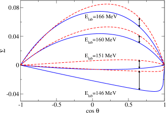
Figure 5: Energy dependence of the photon asymmetry in neutral pion photoproduction from the coupled-channel theory. The solid lines correspond to our calculation with only $s$- and $p$-wave multipoles included. The effect of higher partial waves is shown by the dashed lines.

4 Summary

We reviewed recent progress on a unified description of pion and photon-nucleon scattering up to and beyond the isobar resonance region. A novel scheme that combines causality, unitarity and gauge invariance and that is based on the chiral Lagrangian was discussed. The focus of the talk was the photo-production process with a striking puzzle caused by an old beam asymmetry measurement at MAMI.

References

- Bernard et al. (1995) V. Bernard, N. Kaiser, and U.-G. Meissner, Int. J. Mod. Phys. E4, 193–346 (1995), hep-ph/9501384.
- Bernard (2008) V. Bernard, Prog. Part. Nucl. Phys. 60, 82–160 (2008), 0706.0312.
- Pascalutsa et al. (2007) V. Pascalutsa, M. Vanderhaeghen, and S. N. Yang, Phys. Rept. 437, 125–232 (2007), hep-ph/0609004.
- Bernard et al. (1997) V. Bernard, N. Kaiser, and U.-G. Meissner, Nucl. Phys. A615, 483–500 (1997), hep-ph/9611253.
- Fettes et al. (1998) N. Fettes, U.-G. Meissner, and S. Steininger, Nucl. Phys. A640, 199–234 (1998), hep-ph/9803266.
- Fettes and Meissner (2000) N. Fettes, and U.-G. Meissner, Nucl. Phys. A676, 311 (2000), hep-ph/0002162.
- Bernard et al. (1992) V. Bernard, N. Kaiser, and U. G. Meissner, Nucl. Phys. B383, 442–496 (1992).
- Bernard et al. (1996a) V. Bernard, N. Kaiser, and U.-G. Meissner, Z. Phys. C70, 483–498 (1996a), hep-ph/9411287.
- Bernard et al. (1996b) V. Bernard, N. Kaiser, and U.-G. Meissner, Phys. Lett. B383, 116–120 (1996b), hep-ph/9603278.
- Fearing et al. (2000) H. W. Fearing, T. R. Hemmert, R. Lewis, and C. Unkmeir, Phys. Rev. C62, 054006 (2000), hep-ph/0005213.
- Beane et al. (2005) S. R. Beane, M. Malheiro, J. A. McGovern, D. R. Phillips, and U. van Kolck, Nucl. Phys. A747, 311–361 (2005), nucl-th/0403088.
- Gasparyan and Lutz (2010) A. Gasparyan, and M. F. M. Lutz (2010), 1003.3426.
- MacDowell (1959) S. W. MacDowell, Phys. Rev. 116, 774–778 (1959).
- Mandelstam (1958) S. Mandelstam, Phys. Rev. 112, 1344–1360 (1958).
- Ball (1961) J. S. Ball, Phys. Rev. 124, 2014–2028 (1961).
- Nakanishi (1962) N. Nakanishi, Phys. Rev. 126, 1225–1226 (1962).
- Frazer (1961) W. R. Frazer, Phys. Rev. 123, 2180–2182 (1961).
- Lutz and Kolomeitsev (2002) M. F. M. Lutz, and E. E. Kolomeitsev, Nucl. Phys. A700, 193–308 (2002), nucl-th/0105042.
- Koch (1986) R. Koch, Nucl. Phys. A448, 707 (1986).
- Arndt et al. (2006) R. A. Arndt, W. J. Briscoe, I. I. Strakovsky, and R. L. Workman, Phys. Rev. C74, 045205 (2006), nucl-th/0605082.
- Arndt et al. (2002) R. A. Arndt, W. J. Briscoe, I. I. Strakovsky, and R. L. Workman, Phys. Rev. C66, 055213 (2002), nucl-th/0205067.
- Drechsel et al. (2007) D. Drechsel, S. S. Kamalov, and L. Tiator, Eur. Phys. J. A34, 69–97 (2007), 0710.0306.
- Watson (1954) K. M. Watson, Phys. Rev. 95, 228–236 (1954).
- Bergstrom et al. (1996) J. C. Bergstrom, et al., Phys. Rev. C53, 1052–1056 (1996).
- Schmidt et al. (2001) A. Schmidt, et al., Phys. Rev. Lett. 87, 232501 (2001), nucl-ex/0105010.
- Bernard et al. (1996c) V. Bernard, N. Kaiser, and U.-G. Meissner, Phys. Lett. B378, 337–341 (1996c), hep-ph/9512234.
- Bernard et al. (2001) V. Bernard, N. Kaiser, and U.-G. Meissner, Eur. Phys. J. A11, 209–216 (2001), hep-ph/0102066.
- Schmidt (2001) A. Schmidt, PhD thesis, Mainz (2001), http://wwwa2.kph.uni-maiz.de/A2/ (2001).
- Fernandez-Ramirez et al. (2009) C. Fernandez-Ramirez, A. M. Bernstein, and T. W. Donnelly, Phys. Rev. C80, 065201 (2009), 0907.3463.
- Hanstein et al. (1997) O. Hanstein, D. Drechsel, and L. Tiator, Phys. Lett. B399, 13–21 (1997), nucl-th/9612057.
- Kamalov et al. (2001) S. S. Kamalov, G.-Y. Chen, S.-N. Yang, D. Drechsel, and L. Tiator, Phys. Lett. B522, 27–36 (2001), nucl-th/0107017.