Large-Scale Clustering Based on Data Compression

Abstract

This paper considers the clustering problem for large data sets. We propose an approach based on distributed optimization. The clustering problem is formulated as an optimization problem of maximizing the classification gain. We show that the optimization problem can be reformulated and decomposed into small-scale sub optimization problems by using the Dantzig-Wolfe decomposition method. Generally speaking, the Dantzig-Wolfe method can only be used for convex optimization problems, where the duality gaps are zero. Even though, the considered optimization problem in this paper is non-convex, we prove that the duality gap goes to zero, as the problem size goes to infinity. Therefore, the Dantzig-Wolfe method can be applied here. In the proposed approach, the clustering problem is iteratively solved by a group of computers coordinated by one center processor, where each computer solves one independent small-scale sub optimization problem during each iteration, and only a small amount of data communication is needed between the computers and center processor. Numerical results show that the proposed approach is effective and efficient.

I Introduction

In the recent years, due to the rapid progress of data acquisition and communication technologies, it has become readily easy to collect and store large amounts of data. Large databases of scientific measurements at the scale of terabyte or even petabyte can be frequently observed in high energy physics, astronomy, space exploration and human genome projects. Large databases of financial data and sale transactions at the scale of terabyte or petabyte can also be frequently observed. These huge amounts of data usually contain valuable scientific and business information. For example, a large collection of sale transaction data may contain important information of consumer behaviors and market trends. However, the data analysis on such large databases presents many technique challenges. The database size is usually far larger than the memory size of any single computer. Many existing centralized data analysis algorithms fail for these instances. In fact, most data analysis problems for large databases are currently open or not well-solved.

In this paper, we consider one important data analysis problem, the clustering problem for large databases. The clustering problem is the problem that a set of given data samples are classified into different groups, so that, the data samples within each group are similar according to certain metrics. Clustering is a fundamental problem in data analysis. It has many applications in pattern recognition, machine learning, data mining, computer vision, and signal processing. For example, clustering is usually an important step in many data mining algorithms.

Many algorithms for clustering problems have been previously discussed in the literature, see for example [1] and references therein. These algorithms range from heuristic algorithms to statistical modeling based algorithms. Among the previous algorithms, the statistical modeling based methods generally have better clustering performance compared with other types of algorithms, especially when the data clusters are not well separated. The Expectation-Maximization (EM) algorithms with mixture Gaussian modeling [2] [3] are the major state-of-the-art statistical modeling based clustering algorithms. The EM algorithms can be considered as iterative algorithms for computing the maximum likelihood estimation. It has been proven that the likelihood functions do not decrease during iterations.

However, it is well-known that the EM algorithms have certain limitations. First, according to previous experimental results, the EM algorithms may convergence very slowly [4], [5]. It is shown in [6], that the EM algorithms are first-order optimization algorithms, which provides a theoretical explanation for the slow convergence speeds. In fact, it has been a long-standing open problem that super-linear and second-order methods should be found and preferred for the clustering problems [7]. Second, the EM algorithms do not converge and have numerical difficulties for certain types of instances [4], [8]. For example, the EM algorithms do not converge, when the covariance matrices are singular. The EM algorithms also do not converge, when the numbers of components in the mixture modeling are greater than the actual numbers of data clusters.

In addition, the standard EM algorithms require memory spaces proportional to the database size, therefore, do not scale well. Various scaling-up versions of the standard EM algorithms have been proposed in the literature [9], [10]. However, these previous approaches are approximation algorithms. The accuracy of the obtained results decreases as the ratio between the database size and main processor memory space size increases.

In this paper, we propose a new clustering algorithm for large databases based on data compression principles and mixture Gaussian modeling. Following the approaches in [11], we formulate the clustering problems as optimization problems. Instead of using a centralized approach, we propose a distributed algorithm to solve the global optimization problems. In our approach, the global optimization problem is decomposed into small-scale sub optimization problems using the Dantzig-Wolfe decomposition method [12]. Generally speaking, the Dantzig-wolfe method can only be used in the convex optimization case, where the duality gaps are zero. Even though, the considered problem in this paper is non-convex, we show that the duality gap goes to zeros as the problem size goes to infinity. Therefore, the Dantzig-Wolfe method can be applied here. Our algorithm is especially suitable for the cases of distributed databases, where data are stored at multiple hosts or even at different geographical locations. The global optimal solutions can be computed with only intra-host computations, intra-host local database queries and a small amount of inter-host communications. Unlike many clustering algorithms for large databases, which compute approximate solutions, our algorithm computes exact solutions. Numerical results show that the proposed algorithm does not have any numerical difficulties for the case that the covariance matrices are singular. Numerical results also show that the algorithm has fast convergence speeds.

The rest of this paper is organized as follows. We present the proposed algorithm in Section II. We prove that the duality gap is vanishing for sufficiently large databases in Section III. Numerical results are presented in Section IV. We present the conclusion remark in Section V.

Notation: We use bold face lower-case letters and bold face capital letters to denote the column vectors and matrices respectively. For example, we use $\boldsymbol{a}$ to denote a column vector $\boldsymbol{a}$. We use $\boldsymbol{a}(d)$ to denote the $d$-th element of the vector $\boldsymbol{a}$. We use $\boldsymbol{A}^{t}$ to denote the transpose of the matrix $\boldsymbol{A}$. We use $H(p_{1},\ldots,p_{J})$ to denote the entropy function,

$$H(p_{1},\ldots,p_{J})=\sum_{i=1}^{J}-p_{i}\log\left(p_{i}\right).$$ (1)

We use $\log(x)$ to denote the natural logarithm of the number $x$. We use $det(\boldsymbol{A})$ to denote the determinant of the matrix $\boldsymbol{A}$.

II Clustering Algorithm

In this paper, we consider a data set consisting of $N$ data samples, $\boldsymbol{x}_{1},\boldsymbol{x}_{2},\ldots,\boldsymbol{x}_{N}$, where each data sample is a $D$ dimensional vector. We assume that the data samples are randomly distributed with a mixture Gaussian distribution. That is,

$$p(\boldsymbol{x}_{n})=$$

$$\sum_{i=1}^{J}p_{i}\frac{1}{(2\pi)^{D/2}det(\boldsymbol{\Sigma}_{i})^{1/2}}\exp\left\{-\frac{1}{2}(\boldsymbol{x}_{n}-\boldsymbol{\mu}_{i})^{t}\boldsymbol{\Sigma}_{i}^{-1}(\boldsymbol{x}_{n}-\boldsymbol{\mu}_{i})\right\}$$ (2)

Alternatively, we may consider $\boldsymbol{x}_{1},\ldots,\boldsymbol{x}_{n},\ldots,\boldsymbol{x}_{N}$ as a mixture of data samples from $J$ information sources, where each information source is Gaussian distributed. The considered problem is therefore estimating the membership of each data sample to one of the $J$ information sources, and also the probability distribution of each information source.

In this paper, we propose a distributed algorithm for the above clustering problem. Our algorithm is efficient for the case that the data set contains a large amount of data samples. The data samples can be stored at multiple computers or database hosts. The proposed algorithm formulates the clustering problem as an optimization problem and decomposes the optimization problem into multiple small-scale sub optimization problems. Each sub optimization problem can be solved at one database host using only locally stored data samples. A center processor coordinates the computation at the database hosts. The final solution is obtained from the sub optimization results. A diagram of the system is shown in Fig. 1.

Figure 1: The diagram of the system.

The algorithm in this paper is built up on the data compression based algorithm for clustering in [11]. The main idea behind the algorithm is that optimal data clustering should induce optimal adaptive data compression. That is, if we partition the data set into several clusters and use one data compression encoder for each cluster, then the optimal compression performance is achieved if each cluster contains only the data samples from one information source. The algorithm in [11] then formulates the data cluster problem as an optimization problem, where the classification gain is maximized. The classification gain is a measure of data compression efficiency previously proposed in the data compression literature [13].

If the covariance matrices of all clusters are not singular, then the classification gain is inversely proportional to the following function,

$$2H(p_{1},\ldots,p_{J})+\sum_{i=1}^{J}p_{i}\log\left(det\left(\boldsymbol{\Sigma}_{i}\right)\right)$$ (3)

where, $p_{i}$ is the fraction of data samples in the $i$-th cluster, and $\boldsymbol{\Sigma}_{i}$ is the covariance matrix of the $i$-th cluster. The above function is the objective function in our optimization formulation. In the sequel, we will always assume that the covariance matrices of all clusters are not singular without the loss of generality. Because, if any covariance matrix is singular, we can minimize the following function in the algorithm instead,

$$2H(p_{1},\ldots,p_{J})+\sum_{i=1}^{J}p_{i}\log\left(det\left(\boldsymbol{\Sigma}_{i}+\sigma_{n}^{2}\boldsymbol{I}_{D}\right)\right)$$ (4)

where, $\sigma_{n}^{2}$ is a sufficiently small positive number, and $\boldsymbol{I}_{D}$ is the $D$ dimensional identity matrix. This is equivalent to adding white noise with covariance matrix $\sigma_{n}^{2}\boldsymbol{I}_{D}$ to the data samples and clustering the noise corrupted data samples instead. The optimality of the final obtained clustering results is not much affected, if $\sigma_{n}^{2}$ is small enough.

The proposed algorithm formulates the clustering problem as an optimization problem. We introduce a variable $a_{ni}$ for each $n,i$, $1\leq n\leq N$, and $1\leq i\leq J$. The variable $a_{ni}$ is a likelihood that the $n$-th data sample belongs to the $i$-th information source. The mean $\boldsymbol{\mu}_{i}$, covariance matrix $\boldsymbol{\Sigma}_{i}$, and occurrence probability $p_{i}$ are functions of the likelihood variables $a_{ni}$,

$$\boldsymbol{\mu}_{i}=\frac{\sum_{n=1}^{N}a_{ni}\boldsymbol{x}_{n}}{\sum_{n=1}^{N}a_{ni}}$$ (5)

$$\boldsymbol{\Sigma}_{i}=\left(\frac{1}{\sum_{n=1}^{N}a_{ni}}\right)\sum_{n=1}^{N}a_{ni}(\boldsymbol{x}_{n}-\boldsymbol{\mu}_{i})(\boldsymbol{x}_{n}-\boldsymbol{\mu}_{i})^{t}$$ (6)

$$p_{i}=\frac{\sum_{n=1}^{N}a_{ni}}{N}.$$ (7)

The formulated optimization problem is therefore,

$$\min_{\boldsymbol{a}}\left\{2H(p_{1},\ldots,p_{J})+\sum_{i=1}^{J}p_{i}\log\left(det\left(\boldsymbol{\Sigma}_{i}\right)\right)\right\}$$

$$\mbox{Subject to: }\boldsymbol{a}\in\Omega$$ (8)

where, $\boldsymbol{a}$ is a vector obtained by stacking all the variables $a_{ni}$,

$$\Omega=\left\{\boldsymbol{a}\left|\sum_{i=1}^{J}a_{ni}=1,0\leq a_{ni}\leq 1\right.\right\}.$$ (9)

The final estimation results can be obtained by randomly rounding the optimal solution $a_{ni}^{\ast}$ of the above optimization problem as in [11]. The near-optimality of this optimization based approach has been shown in [11] and [14].

In the sequel, we show that the optimization problem in Eqn. II can be reduced into sub optimization problems that can be locally solved at each database host. The reduction and reformulation procedure consists of four steps.

In the first step of reformulating the problem, we adopt an approach of first solving the restricted optimization problems with $p_{i}$ being fixed,

$$g(\widetilde{p}_{1},\ldots,\widetilde{p}_{J})^{\ast}$$

$$=\min_{\boldsymbol{a}}\left\{2H(\widetilde{p}_{1},\ldots,\widetilde{p}_{J})+\sum_{i=1}^{J}\widetilde{p}_{i}\log\left(det\left(\boldsymbol{\Sigma}_{i}\right)\right)\right\}$$

$$\mbox{Subject to: }\boldsymbol{a}\in\Omega,\mbox{ and }\sum_{n=1}^{N}a_{ni}=\widetilde{p}_{i}N,\mbox{ for all }i,$$ (10)

And then, we optimize over $\widetilde{p}_{1},\ldots,\widetilde{p}_{J}$ to find the overall optimization solution,

$$\min_{\widetilde{p}_{1},\ldots,\widetilde{p}_{J}}g(\widetilde{p}_{1},\ldots,\widetilde{p}_{J})^{\ast},$$

$$\mbox{Subject to: }\sum_{i=1}^{J}\widetilde{p}_{i}=1,0\leq\widetilde{p}_{i}\leq 1.$$ (11)

The problem in Eqn. II can be easily solved by using the gradient descent approach. The main problem is therefore reduced to the optimization problem in Eqn. II.

In the second step of reformulating the problem, we introduce auxiliary unitary matrices $\boldsymbol{A}_{1},\ldots,\boldsymbol{A}_{J}$. We define $\boldsymbol{B}_{i}=\boldsymbol{A}_{i}\boldsymbol{\Sigma}_{i}\boldsymbol{A}_{i}^{t}$, for $i=1,\ldots,J$. It can be shown that the optimization problem in Eqn. II is equivalent to the following optimization problem.

$$\min_{\boldsymbol{A}_{1},\ldots,\boldsymbol{A}_{J},\boldsymbol{a}}\sum_{i=1}^{J}\widetilde{p}_{i}\sum_{d=1}^{D}\log\left(\sigma_{id}^{2}\right),$$

$$\mbox{Subject to: }\boldsymbol{a}\in\Omega,\,\,\,\boldsymbol{A}_{1},\ldots,\boldsymbol{A}_{J}\mbox{ are unitary}$$

$$\sum_{n=1}^{N}a_{ni}=\widetilde{p}_{i}N$$ (12)

where, $\sigma_{id}^{2}$ is the $d$-th diagonal element of the matrix $\boldsymbol{B}_{i}$. The two optimization problems are equivalent, because

$$\sum_{i=1}^{J}\widetilde{p}_{i}\log\left(det\left(\boldsymbol{\Sigma}_{i}\right)\right)\leq\sum_{i=1}^{J}\widetilde{p}_{i}\sum_{d=1}^{D}\log\left(\sigma_{id}^{2}\right)$$ (13)

due to the Hadamard inequality [15, page 502, Thm. 16.8.2], and clearly equality can be achieved by certain $\boldsymbol{A}_{1},\ldots,\boldsymbol{A}_{J}$.

We solve the optimization problem in Eqn. II by an alternating optimization approach. That is, we iteratively first fix $\boldsymbol{A}_{1},\ldots,\boldsymbol{A}_{J}$ and optimize over $\boldsymbol{a}$, and then fix $\boldsymbol{a}$ and optimize over $\boldsymbol{A}_{1},\ldots,\boldsymbol{A}_{J}$. The latter optimization problem is easy to solve, because the optimal $\boldsymbol{A}_{1},\ldots,\boldsymbol{A}_{J}$ are clearly the matrices, such that $\boldsymbol{B}_{i}$ becomes diagonal. The main optimization problem is therefore reduced to

$$\min_{\boldsymbol{a}}\sum_{i=1}^{J}\widetilde{p}_{i}\sum_{d=1}^{D}\log\left(\sigma_{id}^{2}\right),$$

$$\mbox{Subject to: }\boldsymbol{a}\in\Omega,\,\,\,\sum_{n=1}^{N}a_{ni}=\widetilde{p}_{i}N,$$ (14)

where, $\boldsymbol{A}_{1},\ldots,\boldsymbol{A}_{J}$ are fixed and given.

In the third step of reformulating the problem, we use an iterative upper bounding and minimizing approach to solve the optimization problem in Eqn. II. Let $\sigma_{id}^{2}[t]$ denote the solution obtained in the $t$-th iteration. Note that the objective function in Eqn II can be upper bounded as follows, due to the fact that the objective function is concave with respect to $\sigma_{id}^{2}$.

$$\sum_{i=1}^{J}\widetilde{p}_{i}\sum_{d=1}^{D}\log\left(\sigma_{id}^{2}\right)$$

$$\leq\sum_{i=1}^{J}\widetilde{p}_{i}\sum_{d=1}^{D}\log\left(\sigma_{id}^{2}[t]\right)+\sum_{i=1}^{J}\sum_{d=1}^{D}\frac{\widetilde{p}_{i}}{\sigma_{id}^{2}[t]}\left(\sigma_{id}^{2}-\sigma_{id}^{2}[t]\right)$$ (15)

In the $(t+1)$-th iteration, we find a solution $\boldsymbol{a}$, such that the corresponding $\sigma_{id}^{2}$ minimizes the above upper bound. It can be seen clearly that the objective function never increase during iterations. Therefore, the main optimization problem is reduced to the following optimization problem.

$$\min_{\boldsymbol{a}}\left\{\sum_{i=1}^{J}\sum_{d=1}^{D}\widetilde{p}_{i}\beta_{id}\sigma_{id}^{2}\right\}$$

$$\mbox{Subject to: }\boldsymbol{a}\in\Omega,\,\,\,\sum_{n=1}^{N}a_{ni}=\widetilde{p}_{i}N,$$ (16)

where $\beta_{id}=1/\sigma_{id}^{2}[t]$.

In the fourth and final step of reformulating the problem, we decompose the optimization problem in Eqn. II into sub optimization problems by using the Dantzig-Wolfe decomposition method. Each sub optimization problem can be locally solved at each database host. The Dantzig-Wolfe decomposition method is introduced initially for linear programming problems [12]. The method has been then generalized to the convex optimization cases, where the duality gaps are zero, (see for example [16] and references therein). For non-convex optimization problems, the decomposition method generally can not be applied due to the non-zero duality gaps. Even though the optimization problem in Eqn. II is not convex, we show in Theorem III.6 that the duality gap goes to zeros as the number of data samples $N$ goes to infinity. Therefore, the decomposition method can be applied here.

Let us assume that the data samples $\boldsymbol{x}_{1},\ldots,\boldsymbol{x}_{n},\ldots,\boldsymbol{x}_{N}$ are stored at $K$ database hosts. Let ${\mathcal{N}}_{k}$ denote the set of the indexes of the data samples stored at the $k$-th host. We use $\boldsymbol{A}_{i}\boldsymbol{x}_{n}(d)$ to denote the $d$-th element of the vector $\boldsymbol{A}_{i}\boldsymbol{x}_{n}$. The optimization problem in Eqn. II is equivalent to the following optimization problem.

$$\min_{\boldsymbol{a},\boldsymbol{\widehat{\mu}}}\left\{\sum_{i=1}^{J}\sum_{k=1}^{K}\sum_{n\in{\mathcal{N}}_{k}}\sum_{d=1}^{D}\frac{a_{ni}}{N}\beta_{id}\left[\boldsymbol{A}_{i}\boldsymbol{x}_{n}(d)-\widehat{\mu}_{ikd}\right]^{2}\right\}$$

Subject to:

$$\sum_{i=1}^{J}a_{ni}=1,\,\,\,0\leq a_{ni}\leq 1,\,\,\,\sum_{n=1}^{N}a_{ni}/N=\widetilde{p}_{i},$$

$$\widehat{\mu}_{ikd}=\frac{1}{\widetilde{p}_{i}N}\sum_{n=1}^{N}a_{ni}\boldsymbol{A}_{i}\boldsymbol{x}_{n}(d),$$ (17)

where, $\boldsymbol{\widehat{\mu}}$ is the vector obtained by stacking all the variables $\widehat{\mu}_{ikd}$. The real number $\widehat{\mu}_{ikd}$ can be considered as a local guess or estimation of the mean of $\boldsymbol{A}_{i}\boldsymbol{x}_{n}(d)$ at the $k$-th database host. If all the local guesses are equal, then the above objective function is equal to the objective function in Eqn. II.

Because the duality gap is approximately zero as proven in Theorem III.6, the optimization problem in Eqn. II is approximately equivalent to its Lagrangian dual problem as follows.

$$\max_{\boldsymbol{\lambda}}\min_{\boldsymbol{a},\boldsymbol{\widehat{\mu}}}\left\{\sum_{i=1}^{J}\sum_{k=1}^{K}\sum_{n\in{\mathcal{N}}_{k}}\sum_{d=1}^{D}\frac{a_{ni}}{N}\beta_{id}(\boldsymbol{A}_{i}\boldsymbol{x}_{n}(d)-\widehat{\mu}_{ikd})^{2}\right\}$$

$$+\sum_{i=1}^{J}\sum_{k=1}^{K}\sum_{d=1}^{D}\lambda_{\mu ikd}\left(\widehat{\mu}_{ikd}-\frac{1}{\widetilde{p}_{i}N}\sum_{n=1}^{N}a_{ni}\boldsymbol{A}_{i}\boldsymbol{x}_{n}(d)\right)$$

$$+\sum_{i=1}^{J}\lambda_{pi}\left[\sum_{n=1}^{N}a_{ni}/N-\widetilde{p}_{i}\right]$$

$$\mbox{Subject to: }\boldsymbol{a}\in\Omega,$$ (18)

where, $\boldsymbol{\lambda}$ denotes the vector obtained by stacking all variables $\lambda_{\mu ikd}$ and $\lambda_{pi}$. The above optimization problem is separable and can be rewritten as,

$$\max_{\boldsymbol{\lambda}}\sum_{k=1}^{K}f_{k}^{\ast}-\sum_{i=1}^{J}\lambda_{pi}\widetilde{p}_{i},$$ (19)

where, each $f_{k}^{\ast}$ is the optimization result of one sub optimization problem. Let $\boldsymbol{a}_{k}$ denote the vector obtained by stacking all variables $a_{ni}$ with $n\in{\mathcal{N}}_{k}$. Let $\boldsymbol{\widehat{\mu}}_{k}$ denote the vector obtained by stacking all parameters $\widehat{\mu}_{ikd}$, $i=1,\ldots,J$, $d=1,\ldots,D$.

$$f_{k}^{\ast}=\min_{\boldsymbol{a}_{k},\boldsymbol{\widehat{\mu}}_{k}}\left\{\sum_{i=1}^{J}\sum_{n\in{\mathcal{N}}_{k}}\sum_{d=1}^{D}\frac{a_{ni}}{N}\beta_{id}(\boldsymbol{A}_{i}\boldsymbol{x}_{n}(d)-\widehat{\mu}_{ikd})^{2}\right\}$$

$$+\sum_{i=1}^{J}\sum_{d=1}^{D}\lambda_{\mu ikd}\widehat{\mu}_{ikd}+\sum_{i=1}^{J}\lambda_{pi}\sum_{n\in{\mathcal{N}}_{k}}\frac{a_{ni}}{N}$$

$$-\sum_{i=1}^{J}\sum_{k=1}^{K}\sum_{d=1}^{D}\frac{\lambda_{\mu ikd}}{\widetilde{p}N}\sum_{n\in{\mathcal{N}}_{k}}a_{ni}\boldsymbol{A}_{i}\boldsymbol{x}_{n}(d)$$

$$\mbox{Subject to: }\sum_{i=1}^{J}a_{ni}=1,\,\,\,0\leq a_{ni}\leq 1,\mbox{ for }n\in{\mathcal{N}}_{k}.$$ (20)

It can be clearly checked that each $f_{k}^{\ast}$ can be solved locally at each database host using only information about local data samples $\boldsymbol{x}_{n}$, $n\in{\mathcal{N}}_{k}$ with given parameters $\beta_{id}$, $\boldsymbol{\lambda}$, and $\boldsymbol{A}_{1},\ldots,\boldsymbol{A}_{J}$.

Therefore, the proposed algorithm iteratively computes the clustering result. During each iteration, each database host solves one local small-scale optimization problem as in Eqn. II. The center processor then solves the global optimization problem as in Eqn. 19 using the local optimization results. The global optimization problem can be solved by using, for example, the subgradient method [16, Section 6.3.1].

III Vanishing Duality Gap

In this section, we prove that the duality gap between the primal optimization problem in Eqn. II and the dual optimization problem in Eqn. II goes to zero as the problem size $N$ goes to infinity. We need the Azuma inequality in our discussion. A proof of the inequality can be found, for example in [17][18].

Lemma III.1

(Azuma Inequality) Let $Z_{1},\dots,Z_{N}$ be independent random variables, with $Z_{k}$ taking values in a set $\Lambda_{k}$. Assume that a (measurable) function $f:\Lambda_{1}\times\Lambda_{2}\times\cdots\times\Lambda_{N}\rightarrow{\mathbb{R}}$ satisfies the following Lipschitz condition (L).

• (L) If the vectors $z,z^{\prime}\in\prod_{1}^{N}\Lambda_{i}$ differ only in the $k$th coordinate, then $|f(z)-f(z^{\prime})|<c_{k}$, $k=1,\ldots,N$.

Then, the random variable $X=f(Z_{1},\ldots,Z_{N})$ satisfies, for any $t\geq 0$,

$${\mathbb{P}}(X\geq{\mathbb{E}}X+t)\leq\exp\left(\frac{-2t^{2}}{\sum_{1}^{N}c_{k}^{2}}\right),$$ (21)

$${\mathbb{P}}(X\leq{\mathbb{E}}X-t)\leq\exp\left(\frac{-2t^{2}}{\sum_{1}^{N}c_{k}^{2}}\right).$$ (22)

The basic idea is to use randomization. Randomization has been used previously in establishing stronger duality theories. We refer interested readers to [19] and references therein. Let $p(\boldsymbol{a},\boldsymbol{\widehat{\mu}})$ denote the probability distribution of $\boldsymbol{a}$ and $\boldsymbol{\widehat{\mu}}$, where the range of $\boldsymbol{a}$ is $\Omega$, and

$$\min_{n}\boldsymbol{A}_{i}\boldsymbol{x}_{n}(d)\leq\widehat{\mu}_{ikd}\leq\max_{n}\boldsymbol{A}_{i}\boldsymbol{x}_{n}(d).$$ (23)

We introduce the following randomized primal optimization problem.

$$\min_{p(\boldsymbol{a},\boldsymbol{\widehat{\mu}})}{\mathbb{E}}\left\{\sum_{i=1}^{J}\sum_{k=1}^{K}\sum_{n\in{\mathcal{N}}_{k}}\sum_{d=1}^{D}\frac{a_{ni}}{N}\beta_{id}(\boldsymbol{A}_{i}\boldsymbol{x}_{n}(d)-\widehat{\mu}_{ikd})^{2}\right\}$$

Subject to:

$${\mathbb{E}}\left[\left(\widehat{\mu}_{ikd}-\frac{1}{\widetilde{p}_{i}N}\sum_{n=1}^{N}a_{ni}\boldsymbol{A}_{i}\boldsymbol{x}_{n}(d)\right)\right]=0,$$

$${\mathbb{E}}\left[\left.\frac{1}{N}\sum_{n=1}^{N}a_{ni}-\widetilde{p}_{i}\right|\boldsymbol{\widehat{\mu}}\right]=0,\mbox{ for all }\boldsymbol{\widehat{\mu}}.$$ (24)

The corresponding Lagrangian randomized dual problem is

$$\max_{\boldsymbol{\lambda}}\min_{p(\boldsymbol{a},\boldsymbol{\widehat{\mu}})}{\mathbb{E}}\left\{\sum_{i=1}^{J}\sum_{k=1}^{K}\sum_{n\in{\mathcal{N}}_{k}}\sum_{d=1}^{D}\frac{a_{ni}}{N}\beta_{id}(\boldsymbol{A}_{i}\boldsymbol{x}_{n}(d)-\widehat{\mu}_{ikd})^{2}\right\}$$

$$+\int\sum_{i=1}^{J}\lambda_{pi}(\boldsymbol{\widehat{\mu}}){\mathbb{E}}\left[\left.\frac{1}{N}\sum_{n=1}^{N}a_{ni}-\widetilde{p}_{i}\right|\boldsymbol{\widehat{\mu}}\right]d\boldsymbol{\widehat{\mu}}$$

$$+\sum_{i=1}^{J}\sum_{k=1}^{K}\sum_{d=1}^{D}\lambda_{\mu ikd}{\mathbb{E}}\left[\widehat{\mu}_{ikd}-\frac{1}{\widetilde{p}_{i}N}\sum_{n=1}^{N}a_{ni}\boldsymbol{A}_{i}\boldsymbol{x}_{n}(d)\right].$$ (25)

Let us denote the optimal solutions of the primal optimization problem in Eqn. II, randomized primal optimization problem in Eqn. III, dual optimization problem in Eqn. II, and randomized dual optimization problem in Eqn. III by $P^{\ast}$, $PR^{\ast}$, $D^{\ast}$, and $DR^{\ast}$ respectively. We have the following lemmas.

Lemma III.2

$$PR^{\ast}\leq P^{\ast}$$ (26)

Proof:

The lemma follows from the fact that each deterministic variable can be considered as a random variable with a singleton probability distribution. ∎

Lemma III.3

$$DR^{\ast}\leq D^{\ast}$$ (27)

Proof:

Similar as the proof of Lemma III.2. ∎

Lemma III.4

$$PR^{\ast}=DR^{\ast}$$ (28)

Proof:

We may define the following $PR_{\epsilon}$ optimization problem.

$$\min_{p(\boldsymbol{a},\boldsymbol{\widehat{\mu}})}{\mathbb{E}}\left\{\sum_{i=1}^{J}\sum_{k=1}^{K}\sum_{n\in{\mathcal{N}}_{k}}\sum_{d=1}^{D}\frac{a_{ni}}{N}\beta_{id}(\boldsymbol{A}_{i}\boldsymbol{x}_{n}(d)-\widehat{\mu}_{ikd})^{2}\right\}$$ (29)

Subject to:

$$\left|{\mathbb{E}}\left[\left.\frac{1}{N}\sum_{n=1}^{N}a_{ni}-\widehat{p}_{i}\right|\boldsymbol{\widehat{\mu}}\right]\right|\leq\epsilon,\mbox{ for all }\boldsymbol{\widehat{\mu}},$$ (30)

$$\left|\widehat{\mu}_{ikd}-\frac{1}{\widetilde{p}_{i}N}\sum_{n=1}^{N}a_{ni}\boldsymbol{A}_{i}\boldsymbol{x}_{n}(d)\right|\leq\epsilon.$$ (31)

It can be check that $PR_{\epsilon}^{\ast}\leq PR^{\ast}$, and $PR_{\epsilon}^{\ast}\rightarrow PR^{\ast}$, as $\epsilon\rightarrow 0$. The dual of the $PR_{\epsilon}$ problem $DR_{\epsilon}$ is

$$\max_{\boldsymbol{\lambda}^{-},\boldsymbol{\lambda}^{+}}\min_{p(\boldsymbol{a},\boldsymbol{\widehat{\mu}})}{\mathbb{E}}\left\{\sum_{i=1}^{J}\sum_{k=1}^{K}\sum_{n\in{\mathcal{N}}_{k}}\sum_{d=1}^{D}\frac{a_{ni}}{N}\beta_{id}(\boldsymbol{A}_{i}\boldsymbol{x}_{n}(d)-\widehat{\mu}_{ikd})^{2}\right\}$$

$$+\sum_{i=1}^{J}\sum_{k=1}^{K}\sum_{d=1}^{D}\lambda_{\mu ikd}^{-}\left({\mathbb{E}}\left[\widehat{\mu}_{ikd}-\frac{1}{\widetilde{p}_{i}N}\sum_{n=1}^{N}a_{ni}\boldsymbol{A}_{i}\boldsymbol{x}_{n}(d)\right]-\epsilon\right)$$

$$+\sum_{i=1}^{J}\sum_{k=1}^{K}\sum_{d=1}^{D}(-1)\lambda_{\mu ikd}^{+}\left({\mathbb{E}}\left[\widehat{\mu}_{ikd}-\frac{1}{\widetilde{p}_{i}N}\sum_{n=1}^{N}a_{ni}\boldsymbol{A}_{i}\boldsymbol{x}_{n}(d)\right]+\epsilon\right)$$

$$+\int\sum_{i=1}^{J}\lambda_{pi}^{-}(\boldsymbol{\widehat{\mu}})\left\{{\mathbb{E}}\left[\left.\frac{1}{N}\sum_{n=1}^{N}a_{ni}-\widetilde{p}_{i}\right|\boldsymbol{\widehat{\mu}}\right]-\epsilon\right\}d\boldsymbol{\widehat{\mu}}$$

$$+\int\sum_{i=1}^{J}(-1)\lambda_{pi}^{+}(\boldsymbol{\widehat{\mu}})\left\{{\mathbb{E}}\left[\left.\frac{1}{N}\sum_{n=1}^{N}a_{ni}-\widehat{p}_{i}\right|\boldsymbol{\widehat{\mu}}\right]+\epsilon\right\}d\boldsymbol{\widehat{\mu}}$$

$$\mbox{Subject to: }\lambda_{\mu ikd}^{-}\geq 0,\lambda_{\mu ikd}^{+}\geq 0,\lambda_{pi}^{-}(\boldsymbol{\widehat{\mu}})\geq 0,\lambda_{pi}^{+}(\boldsymbol{\widehat{\mu}})\geq 0.$$ (32)

It can be also checked that $DR_{\epsilon}^{\ast}\rightarrow DR^{\ast}$, as $\epsilon\rightarrow 0$.

Now we show that $PR_{\epsilon}$ is a convex optimization problem. Let $p^{1}(\boldsymbol{a},\boldsymbol{\widehat{\mu}})$, $p^{2}(\boldsymbol{a},\boldsymbol{\widehat{\mu}})$ be two probability distributions satisfying all the constraints in the $PR_{\epsilon}$ problem. Let

$$p(\boldsymbol{a},\boldsymbol{\widehat{\mu}})=\alpha p^{1}(\boldsymbol{a},\boldsymbol{\widehat{\mu}})+(1-\alpha)p^{2}(\boldsymbol{a},\boldsymbol{\widehat{\mu}}),$$ (33)

where, $0\leq\alpha\leq 1$. Equivalently, we may introduce a random variable $z$, ${\mathbb{P}}(z=1)=\alpha$, ${\mathbb{P}}(z=2)=1-\alpha$; $p(\boldsymbol{a},\boldsymbol{\widehat{\mu}})=p^{1}(\boldsymbol{a},\boldsymbol{\widehat{\mu}})$, if $z=1$, and $p(\boldsymbol{a},\boldsymbol{\widehat{\mu}})=p^{2}(\boldsymbol{a},\boldsymbol{\widehat{\mu}})$, if $z=2$. We can show that $p(\boldsymbol{a},\boldsymbol{\widehat{\mu}})$ satisfies the constraint in Eqn. 30 as follows.

$${\mathbb{E}}\left[\left.\sum_{n=1}^{N}\frac{a_{ni}}{N}-\widehat{p}_{i}\right|\boldsymbol{\widehat{\mu}}\right]=\int\left[\sum_{n=1}^{N}\frac{a_{ni}}{N}-\widehat{p}_{i}\right]p(\boldsymbol{a}|\boldsymbol{\widehat{\mu}})d\boldsymbol{a}$$

$$=\int\left[\sum_{n=1}^{N}\frac{a_{ni}}{N}-\widehat{p}_{i}\right]p(\boldsymbol{a},z=1|\boldsymbol{\widehat{\mu}})d\boldsymbol{a}$$

$$\hskip 14.45377pt+\int\left[\sum_{n=1}^{N}\frac{a_{ni}}{N}-\widehat{p}_{i}\right]p(\boldsymbol{a},z=2|\boldsymbol{\widehat{\mu}})d\boldsymbol{a}$$

$$=\int\left[\sum_{n=1}^{N}\frac{a_{ni}}{N}-\widehat{p}_{i}\right]p^{1}(\boldsymbol{a}|\boldsymbol{\widehat{\mu}})p(z=1|\boldsymbol{\widehat{\mu}})d\boldsymbol{a}$$

$$\hskip 14.45377pt+\int\left[\sum_{n=1}^{N}\frac{a_{ni}}{N}-\widehat{p}_{i}\right]p^{2}(\boldsymbol{a}|\boldsymbol{\widehat{\mu}})p(z=2|\boldsymbol{\widehat{\mu}})d\boldsymbol{a}$$

$$\leq p(z=1|\boldsymbol{\widehat{\mu}})\epsilon+p(z=2|\boldsymbol{\widehat{\mu}})\epsilon\,\,\,\leq\epsilon$$ (34)

Similarly,

$${\mathbb{E}}\left[\left.\sum_{n=1}^{N}\frac{a_{ni}}{N}-\widehat{p}_{i}\right|\boldsymbol{\widehat{\mu}}\right]\geq\epsilon$$ (35)

We can also show that $p(\boldsymbol{a},\boldsymbol{\widehat{\mu}})$ satisfies the constraint in Eqn. 31 by using the fact that the expectation is a linear functional. Finally, the objective function in Eqn. 29 is also convex, because the expectation is a linear functional. Therefore, the optimization problem $PR_{\epsilon}$ is a convex optimization problem.

Because, $PR_{\epsilon}$ is a convex optimization problem and the Slater condition holds, $PR_{\epsilon}^{\ast}=DR_{\epsilon}^{\ast}$ according to the strong duality theorem [20, Thm. 6.7]. Therefore, $PR^{\ast}=DR^{\ast}$. ∎

Lemma III.5

Assume $\max_{n,m}||\boldsymbol{x}_{n}-\boldsymbol{x}_{m}||_{2}\leq V$, for a fixed upper bound $V$, where $||\cdot||_{2}$ denotes the Euclidean norm. Then $PR^{\ast}\rightarrow P^{\ast}$, as $N$ goes to infinity.

Proof:

Let $p^{\ast}(\boldsymbol{a},\boldsymbol{\widehat{\mu}})$ denote the optimal solution of the randomized primal problem. We can construct a probability distribution $\widehat{p}(\boldsymbol{a},\boldsymbol{\widehat{\mu}})$ as follows.

$$\widehat{p}(\boldsymbol{a},\boldsymbol{\widehat{\mu}})=p^{\ast}(\boldsymbol{\widehat{\mu}})\prod_{n=1}^{N}p^{\ast}(a_{n1},\ldots,a_{nJ}|\boldsymbol{\widehat{\mu}}),$$ (36)

where, the probability distributions at the right hand are marginal distributions. It can be checked that the probability $\widehat{p}(\boldsymbol{a},\boldsymbol{\widehat{\mu}})$ achieves the exactly same objective function and constraint function values in the randomized primal problem as the probability distribution $p^{\ast}(\boldsymbol{a},\boldsymbol{\widehat{\mu}})$. Therefore, we can assume that $p^{\ast}(\boldsymbol{a},\boldsymbol{\widehat{\mu}})$ takes the form in Eqn. 36 without the loss of generality.

We define the typical set ${\mathcal{T}}(\epsilon)$ as

$${\mathcal{T}}(\epsilon)=\left\{(\boldsymbol{a},\boldsymbol{\widehat{\mu}})\left|\left|\sum_{n=1}^{N}\frac{a_{ni}}{N}-\widetilde{p}_{i}\right|\leq\epsilon,\mbox{ for all }i\right.\right\}.$$ (37)

The probability that $(\boldsymbol{a},\boldsymbol{\widehat{\mu}})$ is not in the typical set ${\mathcal{T}}(\epsilon)$ can be upper bounded by using the Azuma inequality and the union bound as follows.

$${\mathbb{P}}\left[(\boldsymbol{a},\boldsymbol{\widehat{\mu}})\notin{\mathcal{T}}(\epsilon)\right]\leq\sum_{i=1}^{J}{\mathbb{P}}\left[\left|\sum_{n=1}^{N}\frac{a_{ni}}{N}-\widetilde{p}_{i}\right|\geq\epsilon\right]$$

$$\leq\sum_{i=1}^{J}\int{\mathbb{P}}\left[\left.\left|\sum_{n=1}^{N}\frac{a_{ni}}{N}-\widetilde{p}_{i}\right|\geq\epsilon\right|\boldsymbol{\widehat{\mu}}\right]p(\boldsymbol{\widehat{\mu}})d\boldsymbol{\widehat{\mu}}$$

$$\leq\sum_{i=1}^{J}\int 2\exp\left(-2\epsilon^{2}N\right)p(\boldsymbol{\widehat{\mu}})d\boldsymbol{\widehat{\mu}}$$

$$\leq 2J\exp\left(-2\epsilon^{2}N\right)$$ (38)

Due to the fact that the objective function is non-negative, the average achieved objective function values by $(\boldsymbol{a},\boldsymbol{\widehat{\mu}})$ in the typical set,

$${\mathbb{E}}\left\{\left.\sum_{i=1}^{J}\sum_{k=1}^{K}\sum_{n\in{\mathcal{N}}_{k}}\sum_{d=1}^{D}\frac{\widehat{a}_{ni}}{N}\beta_{id}(\boldsymbol{A}_{i}\boldsymbol{x}_{n}(d)-\widehat{\mu}_{ikd})^{2}\right|{\mathcal{T}}(\epsilon)\right\}$$

$$\leq\frac{PR^{\ast}}{{\mathbb{P}}((\boldsymbol{a},\boldsymbol{\widehat{\mu}})\in{\mathcal{T}}(\epsilon))}$$ (39)

Also by the above discussions,

$${\mathbb{P}}\left[(\boldsymbol{a},\boldsymbol{\widehat{\mu}})\in{\mathcal{T}}(\epsilon)\right]\geq 1-2J\exp\left(-2\epsilon^{2}N\right)$$ (40)

Therefore, we have that the average of the objective function in the typical set is bounded by

$${\mathbb{E}}\left\{\left.\sum_{i=1}^{J}\sum_{k=1}^{K}\sum_{n\in{\mathcal{N}}_{k}}\sum_{d=1}^{D}\frac{\widehat{a}_{ni}}{N}\beta_{id}(\boldsymbol{A}_{i}\boldsymbol{x}_{n}(d)-\widehat{\mu}_{ikd})^{2}\right|{\mathcal{T}}(\epsilon)\right\}$$

$$\leq\frac{PR^{\ast}}{1-2J\exp(-2\epsilon^{2}N)}$$ (41)

There must exist one $(\boldsymbol{\widehat{a}},\boldsymbol{\bar{\mu}})$ in the typical set, such that the corresponding objective function is less than or equal to the above average. We can further modify the above $\boldsymbol{\widehat{a}}$ into a certain $\boldsymbol{\widetilde{a}}\in\Omega$, $\boldsymbol{\widetilde{a}}=(\ldots,\widetilde{a}_{ni},\ldots)$, such that

$$\sum_{n=1}^{N}\widetilde{a}_{ni}/N=\widetilde{p}_{i},$$ (42)

and the corresponding objective function is raised by at most $(J-1)\max\{\beta_{id}\}V^{2}\epsilon$. We can now set

$$\widetilde{\mu}_{ikd}=\frac{1}{\widetilde{p}_{i}N}\sum_{n=1}^{N}\widetilde{a}_{ni}\boldsymbol{A}_{i}\boldsymbol{x}_{n}(d).$$ (43)

Clearly, $\widetilde{a}_{ni}$ and $\widetilde{\mu}_{ikd}$ satisfy all the constraints in the primal problem. Therefore,

$$P^{\ast} {\leq}\sum_{i=1}^{J}\sum_{k=1}^{K}\sum_{n\in{\mathcal{N}}_{k}}\sum_{d=1}^{D}\frac{\widetilde{a}_{ni}}{N}\beta_{id}\left[(\boldsymbol{A}_{i}\boldsymbol{x}_{n}(d)-\widetilde{\mu}_{ikd})^{2}\right]$$

$$\stackrel{{\scriptstyle(a)}}{{\leq}}\sum_{i=1}^{J}\sum_{k=1}^{K}\sum_{n\in{\mathcal{N}}_{k}}\sum_{d=1}^{D}\frac{\widetilde{a}_{ni}}{N}\beta_{id}(\boldsymbol{A}_{i}\boldsymbol{x}_{n}(d)-\bar{\mu}_{ikd})^{2}$$

$$\leq\frac{PR^{\ast}}{1-2J\exp(-2\epsilon^{2}N)}+(J-1)\max\{\beta_{i}\}V^{2}\epsilon$$ (44)

where, (a) follows from the fact that $\widetilde{\mu}_{ikd}$ are the minimizer of the above quadratic function. The lemma then follows from the fact that $PR^{\ast}\leq P^{\ast}$. ∎

Theorem III.6

The duality gap $P^{\ast}-D^{\ast}$ between the primal problem and dual problem goes to zero as the data sample number $N$ goes to infinity.

IV Numerical Results

In this section, we present numerical results for the proposed clustering algorithm. In Fig. 2, we depict the result of the proposed algorithm for the case of two overlapping clusters in a two dimensional space. Both the two clusters have zero mean. Their covariance matrices are as follows.

$$\left[\begin{array}[]{cc}80000&52000\\ 52000&35600\end{array}\right],\,\,\,\left[\begin{array}[]{cc}192800&-118800\\ -118800&74000\end{array}\right].$$ (49)

The total data sample number is $2048$ and each cluster contains $1024$ data samples. We assume that the data samples can be observed by two database hosts, where the first database host can only observe the $1024$ data samples from the first cluster, and the second database host can only observe the $1024$ data samples from the second cluster. After the clustering result is obtained, we randomly select $128$ data samples from the first cluster and $128$ data samples from the second cluster and plot these data samples in the figure. The data samples classified into one cluster are plotted as red circles and the data sample classified into the other cluster are plotted as blue squares. The percentage of missed classified data samples is $5.32\%$. The clustering errors mainly occur at the regions where the two clusters overlap. The algorithm starts with two randomly selected unitary matrices $\boldsymbol{A}_{1}$, and $\boldsymbol{A}_{2}$. We observe that these matrices converge quickly. We also experiment with the cases that each database host observes a mixture of data samples from the two clusters with various percentages. The obtained results are not significantly different from the result in Fig. 2.

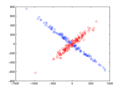
Figure 2: Clustering results for two overlapping clusters.

In Fig. 3, we depict the result of the proposed algorithm for the case of two overlapping clusters with one cluster having a singular covariance matrix. Both the two clusters have zero mean. Their covariance matrices are as follows.

$$\left[\begin{array}[]{cc}80000&52000\\ 52000&35600\end{array}\right],\,\,\,\left[\begin{array}[]{cc}192800&0\\ 0&0\end{array}\right].$$ (54)

The total data sample number is $2048$ and each cluster contains $1024$ data samples. There are two database hosts, and the first database host can only observe the $1024$ data samples from the first cluster, and the second database host can only observe the $1024$ data samples from the second cluster. In the formulated optimization problem, a term $\sigma_{n}^{2}\boldsymbol{I}_{2}$, $\sigma_{n}^{2}=0.5$, is added to the objective function. The clustering results of randomly selected $256$ data samples are shown in the figure. The percentage of missed classified data samples is $1.71\%$. The results for the cases that each database host observes a mixture of data samples from the two clusters with various percentages are not significantly different from the result in the figure. The proposed clustering algorithm does not have any numerical or convergence difficulties for these cases.

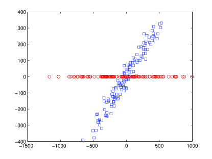
Figure 3: Clustering result for the case that one cluster has a singular covariance matrix.

In Fig. 4, we depict the result of the proposed algorithm for the case of two clusters with different means. The first cluster has zero mean and covariance matrix

$$\left[\begin{array}[]{cc}80000&52000\\ 52000&35600\end{array}\right].$$ (57)

The second cluster has mean $[800,800]^{t}$ and covariance matrix

$$\left[\begin{array}[]{cc}192800&-118800\\ -118800&74000\end{array}\right].$$ (60)

The total data sample number is $2048$ and each cluster contains $1024$ data samples. There are two database hosts, the first database host can only observe the $1024$ data samples from the first cluster, and the second database host can only observe the $1024$ data samples from the second cluster. The percentage of missed classified data samples is $2.29\%$. The results for the cases that each database host observes a mixture of data samples from the two clusters with various percentages are not significantly different from the result in the figure.

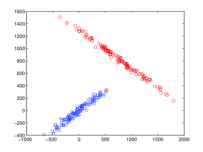
Figure 4: Clustering result for the case that the two clusters have different means.

In summary, we find that the proposed clustering algorithm has low missed classification probability and fast convergence speeds. The algorithm does not have numerical or convergence difficulties for the case of singular covariance matrices. The proposed algorithm is a promising approach for future large-scale data analysis.

V Conclusion

This paper proposes a large-scale data clustering algorithm based on distributed optimization. We show that the duality gap of the considered optimization problem goes to zero as the problem size goes to infinity. Therefore, the global optimization problem can be decomposed into small-scale sub optimization problems by using the Dantzig-Wolfe method. The small-scale sub optimization problems can be solved using a group of computers coordinated by one center processor. Numerical results show that the proposed algorithm is effective, efficient and does not have numerical or convergence difficulties.

References

• [1] A. Jain, M. Murty, and P. Flynn, “Data clustering: A review,” ACM Computing Surveys, vol. 31, no. 3, pp. 264–323, 1999.
• [2] A. Dempster, N. Laird, and D. Rubin, “Maximum likelihood from incomplete data via the EM algorithm,” Journal of the Royal Statistical Society, Series B, vol. 39, no. 1, pp. 1–38, 1977.
• [3] P. Cheeseman and J. Stutz, “Bayesian classification (AutoClass): theory and result,” in Advances in knowledge discovery and data mining, MIT Press, 1996.
• [4] C. Archambeau, J. Lee, and M. Verleysen, “On convergence problems of the EM algorithm for finite Gaussian mixtures,” Proceedings of European Symposium on Artificial Neural Networks, Bruges, Belgium, pp. 99–106, April 2003.
• [5] Z. Yang and S. Chen, “Robust maximum likelihood training of heteroscedastic probabilistic neural networks,” Neural Networks, vol. 11, no. 4, pp. 739–747, June 1998.
• [6] L. Xu and M. Jordan, “On convergence properties of the EM algorithm for Gaussian mixtures,” Neural Computation, vol. 8, no. 1, pp. 129–151, January 1996.
• [7] R. A. Redner and H. F. Walker, “Mixture densities, maximum likelihood and the EM algorithm,” SIAM Review, vol. 26, no. 2, pp. 195–239, April 1984.
• [8] C. Fraley and A. E. Raftery, “How many clusters? which clustering method? answers via model-based cluster analysis,” The Computer Journal, vol. 41, no. 8, pp. 578–589, 1998.
• [9] P. Bradley, U. Fayyad, and C. Reina, “Scaling clustering to large databases,” Proceedings of the Fourth International Conference on Knowledge Discovery and Data Mining, August 1998.
• [10] T. Zhang, R. Ramakrishnan, and M. Livny, “BIRCH: an efficient data clustering method for very large databases,” ACM SIGMOD record, vol. 25, no. 2, pp. 103–114, June 1996.
• [11] X. Ma, “Novel blind signal classification method based on data compression,” in Proceedings of the 6th International Conference on Information Technology: New Generations, Las Vegas, Nevada, USA, April 2009.
• [12] G. Dantzig and P. Wolfe, “Decomposition principle for linear programs,” Operations Research, vol. 8, pp. 101–111, 1960.
• [13] R. Joshi, H. Jafarkhani, J. Kasner, T. Fischer, N. Farvardin, M. Marcellin, and R. Bamberger, “Comparison of different methods of classification in subband coding of images,” IEEE Transactions on Image Processing, vol. 6, no. 11, pp. 1473–1486, November 1997.
• [14] X. Ma. (2010) Performance analysis for data compression based signal classification methods. Internet draft. [Online]. Available: http://arxiv.org/abs/1001.1808
• [15] T. cover and J. Thomas, Elements of Information Theory.   John Wiley & Sons, 1991.
• [16] D. P. Bertsekas, Nonlinear Programming.   Athena Scientific, 1999.
• [17] K. Azuma, “Weighted sums of certain dependent random variables,” Tohoku Mathematical Journal, vol. 19, no. 3, pp. 357–367, 1967.
• [18] S. Janson, “On concentration of probability,” Proceedings of Workshop on Probabilistic Combinatorics at the Paul Erdos Summer Research Center, Budapest, pp. 289–301, 1998.
• [19] Y. Ermoliev, A. Gaivoronski, and C. Nedeva, “Stochastic optimization problems with incomplete information on distribution functions,” SIAM Journal on Control and Optimization, vol. 23, no. 5, pp. 697–716, 1985.
• [20] J. Jahn, Introduction to the Theory of Nonlinear Optimization, 3rd edition.   Springer, 2007.