HELAS and MadGraph with spin-3/2 particles

Abstract

Fortran subroutines to calculate helicity amplitudes with massive spin-3/2 particles, such as massive gravitinos, which couple to the standard model and supersymmetric particles via the supercurrent, are added to the HELAS (HELicity Amplitude Subroutines) library. They are coded in such a way that arbitrary amplitudes with external gravitinos can be generated automatically by MadGraph, after slight modifications. All the codes have been tested carefully by making use of the gauge invariance of the helicity amplitudes.

KEK-TH-1417
HD-THEP-10-20

1 Introduction

Gravitinos are spin-3/2 superpartners of gravitons in local supersymmetric extensions to the Standard Model (SM). If supersymmetry (SUSY) breaks spontaneously, gravitinos absorb massless spin-1/2 goldstinos and become massive by the super-Higgs mechanism. Therefore, the gravitino mass is related to the scale of SUSY breaking as well as the Planck scale like

$$m_{3/2}\sim(M_{\rm SUSY})^{2}/M_{\rm Pl}.$$ (1)

This implies that the gravitino can take a wide range of mass, depending on the SUSY breaking scale, from eV up to scales beyond TeV, and provide rich phenomenology in particle physics as well as in cosmology Giudice:1998bp .

Although the gravitino can play an important role even in collider signatures when it is the lightest supersymmetric particle (LSP), there is few Monte Carlo event generators which can treat them. In this paper, we present new HELAS subroutines Hagiwara:1990dw for the massive gravitinos and their interactions based on the effective Lagrangian below, and implement them into MadGraph/MadEvent (MG/ME) v4 Stelzer:1994ta ; Maltoni:2002qb ; Alwall:2007st so that arbitrary amplitudes with external gravitinos can be generated automatically.

The effective interaction Lagrangian relevant to the gravitino phenomenology is Wess:1992cp ; Moroi:1995fs ; Bolz:2000fu

$${\cal L}_{\rm int}= -\frac{i}{\sqrt{2}\,\overline{M}_{\rm Pl}}$$

$$\ \times\big{[}\bar{\psi}_{\mu}\gamma^{\nu}\gamma^{\mu}P_{L}f^{i}\,(D_{\nu}\phi^{i}_{L})^{*}-\bar{f^{i}}P_{R}\gamma^{\mu}\gamma^{\nu}\psi_{\mu}\,(D_{\nu}{\phi}^{i}_{L})$$

$$\ \ -\bar{\psi}_{\mu}\gamma^{\nu}\gamma^{\mu}P_{R}f^{i}\,(D_{\nu}\phi^{i}_{R})^{*}+\bar{f^{i}}P_{L}\gamma^{\mu}\gamma^{\nu}\psi_{\mu}\,(D_{\nu}{\phi}^{i}_{R})\big{]}$$

$$-\frac{i}{8\overline{M}_{\rm Pl}}\bar{\psi}_{\mu}[\gamma^{\nu},\gamma^{\rho}]\gamma^{\mu}\lambda^{(\alpha)a}F_{\nu\rho}^{(\alpha)a},$$ (2)

where $\psi^{\mu}$ is the spin-3/2 gravitino field, $f^{i}$ and $\phi^{i}$ are spinor and scalar fields in the same chiral supermultiplet, $P_{R/L}=\frac{1}{2}(1\pm\gamma_{5})$ is the chiral-projection operator, and $\overline{M}_{\rm Pl}\equiv M_{\rm Pl}/\sqrt{8\pi}\sim 2.4\times 10^{18}$ GeV is the reduced Planck mass. The covariant derivative is

$$D_{\mu}=\partial_{\mu}+ig_{s}T^{a}_{3}A_{\mu}^{a}+igT^{a}_{2}W_{\mu}^{a}+ig^{\prime}YB_{\mu},$$ (3)

where $g_{s}$, $g$ and $g^{\prime}$ are the $SU(3)_{C}$, $SU(2)_{L}$ and $U(1)_{Y}$ gauge couplings, respectively, and $T^{a}_{3}$, $T^{a}_{2}$ and $Y$ are the generators of the $SU(3)_{C}$ $(a=1,\cdots,8)$, $SU(2)_{L}$ $(a=1,2,3)$ and $U(1)_{Y}$ groups. The field-strength tensors for each gauge group are

$$F_{\mu\nu}^{(3)a} =\partial_{\mu}A_{\nu}^{a}-\partial_{\nu}A_{\mu}^{a}-g_{s}f_{3}^{abc}A_{\mu}^{b}A_{\nu}^{c},$$ (4)

$$F_{\mu\nu}^{(2)a} =\partial_{\mu}W_{\nu}^{a}-\partial_{\nu}W_{\mu}^{a}-gf_{2}^{abc}W_{\mu}^{b}W_{\nu}^{c},$$ (5)

$$F_{\mu\nu}^{(1)a} =\partial_{\mu}B_{\nu}-\partial_{\nu}B_{\mu},$$ (6)

and the corresponding gauginos $\lambda^{(\alpha=3,2,1)a}$ are gluinos ($\tilde{g}^{a}$), winos ($\tilde{W}^{a}$) and bino ($\tilde{B}$), respectively.

The paper is organized as follows: In Sect. 2 we give sample numerical results. Sect. 3 presents our brief summary. In App. A we give the new HELAS subroutines for spin-3/2 particles, and in App. B we describe how to implement the amplitudes into MG.

2 Sample results

In this section, we present some sample numerical results, using the new HELAS subroutines, which are presented in Appendix A, and the modified MG, which is described in Appendix B.

In the gauge mediated SUSY breaking scenarios, the gravitino is often the LSP, and its phenomenology depends on what is the next-to-lightest supersymmetric particle (NLSP). Here we consider the stau NLSP scenario as well as the neutralino NLSP one.

2.1 Stau NLSP

As a sample result for the stau NLSP scenario, we consider radiative $\tilde{\tau}$ decays,

$$\tilde{\tau}_{R}^{-}\rightarrow\tau^{-}\,\tilde{G}\,\gamma.$$ (7a)

Here we regard the stau as a purely right-handed stau for simplicity. Feynman diagrams shown in Fig. 1 and the corresponding helicity amplitudes are generated automatically by the modified MG. To study the spin-3/2 nature of the gravitino, we compare the $$\tilde{G} \tilde{\chi}^{0}_{1}$$ LSP case (7a) with the LSP case,

$$\tilde{\tau}_{R}^{-}\rightarrow\tau^{-}\,\tilde{\chi}^{0}_{1}\,\gamma,$$ (7b)

where only two decay diagrams contribute; see Fig. 2.

Figure 1: Feynman diagrams for the radiative stau decay process for the $\tilde{G}$ LSP case, $\tilde{\tau}\rightarrow\tau\tilde{G}\gamma$, generated by MadGraph. ta1, ta, G$\sim$, A, and Ni denote a stau, a tau-lepton, a gravitino, a photon, and neutralinos, respectively.

Figure 2: The same as Fig. 1, but for the $\tilde{\chi}^{0}_{1}$ LSP case, $\tilde{\tau}\rightarrow\tau\tilde{\chi}^{0}_{1}\gamma$.

We evaluate the amplitudes for the both cases, (7a) and (7b), in the $\tilde{\tau}$ rest frame as

$$p_{\tilde{\tau}} =(m_{\tilde{\tau}},0,0,0),$$

$$p_{\gamma} =(E_{\gamma},0,0,E_{\gamma}),$$

$$p_{\tau} =(E_{\tau},p_{\tau}\sin\theta,0,p_{\tau}\cos\theta),$$

$$p_{\rm LSP} =(E,p^{x},0,p^{z}),$$ (8)

where the $z$-axis is taken along the photon momentum direction, and the $y$-axis is along $\overrightarrow{p}_{\gamma}\times\overrightarrow{p}_{\tau}$, the normal of the decay plane.

Using the generated helicity amplitudes and the above kinematical variables, we investigate photon polarizations by means of Stokes parameters, $P_{1},P_{2}$, and $P_{3}$, which are related with the photon density matrix as

$$\frac{d\rho_{\lambda\lambda^{\prime}}}{dE_{\gamma}\,d\cos\theta}=\frac{1}{2}\left(1+\sum^{3}_{i=1}P_{i}\sigma_{i}\right)_{\lambda\lambda^{\prime}}\cdot\frac{d\Gamma_{\rm sum}}{dE_{\gamma}\,d\cos\theta}$$ (9)

with the Pauli sigma matrices $\sigma_{i}$. $d\Gamma_{\rm sum}=d\rho_{++}+d\rho_{--}$ is the usual spin-summed differential decay rate. The density matrix is calculated as

$$d\rho_{\lambda\lambda^{\prime}}=\frac{1}{2m_{\tilde{\tau}}}\sum{\cal M}_{\lambda}{\cal M}^{*}_{\lambda^{\prime}}\,d\Phi_{3},$$ (10)

where ${\cal M}_{\lambda}$ is the helicity amplitude with the photon helicity $\lambda$, and $d\Phi_{3}$ is the three-body phase space factor. The summation symbol implies the summation over the tau and gravitino/neutralino helicities. By definition, Stokes parameters take real values from $-1$ to $1$, and $P_{3}$ shows the right-left asymmetry of circular polarizations, while $P_{1}$ and $P_{2}$ present linear polarizations, which reflect the interference between the amplitudes for the right- and left-handed photons.

In Fig. 3, we show the $\cos\theta$ dependence of the Stokes parameters of the radiated photon for $\tilde{\tau}_{R}\rightarrow\tau\tilde{G}\gamma$ (a) and $\tilde{\tau}_{R}\rightarrow\tau\tilde{\chi}_{1}^{0}\gamma$ (b), where we use

$$m_{\tilde{\tau}}=150\ {\rm GeV}\ {\rm and}\ m_{\rm LSP}=75\ {\rm GeV},$$ (11)

and fix the photon energy at

$$E_{\gamma}=40\ {\rm GeV}.$$ (12)

For the $\tilde{G}$ LSP scenario (a), we take four neutralino masses as $m_{\tilde{\chi}_{1,2,3,4}^{0}}=(200,250,300,350)$ GeV as an example. The degree of polarization $P=\sqrt{P_{1}^{2}+P_{2}^{2}+P_{3}^{2}}$ is also shown with a thick line. Radiated photons are almost fully polarized ($P\sim 1$) for the both LSP scenarios, except around $\cos\theta=-0.95$ for the $\tilde{G}$ LSP scenario, where photons are close to being unpolarized ($P\sim 0$).

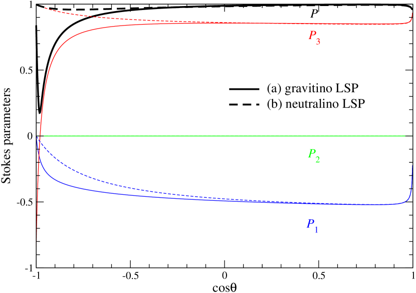
Figure 3: Angular dependence of the Stokes parameters of the radiated photon for the $\tilde{\tau}$ decay process, $\tilde{\tau}_{R}\rightarrow\tau\tilde{G}\gamma$ (a) and $\tilde{\tau}_{R}\rightarrow\tau\tilde{\chi}_{1}^{0}\gamma$ (b), where $\theta$ is the decay angle between the photon and the tau-lepton. We set $m_{\tilde{\tau}}=150$ GeV, $m_{\rm LSP}=75$ GeV and $E_{\gamma}=40$ GeV.

In the $\cos\theta>0$ region, the photon bremsstrahlung amplitude (graph 2 in Figs. 1 and 2) is dominant and the $\tilde{G}$-LSP and $\tilde{\chi}_{1}^{0}$-LSP cases are very similar since only $\pm 1/2$-helicity states of the gravitino are allowed. In the $\cos\theta<0$ region, on the other hand, the neutralino propagating amplitudes and the four-point interaction amplitude, graph 3 to 7 in Fig. 1, become important, which allow the gravitino to take $\pm 3/2$ helicities as well. Note that the amplitude corresponding to the graph 1 in Figs. 1 and 2 always vanishes. Since the gravitino has the large mass in this example, spin-3/2 components dominate spin-1/2 ones, and $P_{3}$ for the $\tilde{G}$ LSP shows distinct behavior from those for the $\tilde{\chi}_{1}^{0}$ LSP. Especially, for $\cos\theta\sim-1$, the difference is significant; $P_{3}=-0.8$ (almost left-handed photon) for the $\tilde{G}$ LSP, while $P_{3}=+1$ (right-handed photon) for the $\tilde{\chi}_{1}^{0}$ LSP. Those behavior holds for heavier neutralinos and agrees with the results of Ref. Buchmuller:2004rq , where the neutralino intermediate diagrams are neglected.

Since the photon helicity measurements require a polarized detector, we also examine linear polarizations $P_{1}$ and $P_{2}$. In both scenarios, the linear polarization perpendicular to the decay plane vanishes ($P_{2}=0$), and $P_{1}$ tends to behave similarly, but slightly larger $|P_{1}|$ is expected in the backward direction ($\cos\theta<0$) for the gravitino LSP case (a).

2.2 Neutralino NLSP

As a sample result for the neutralino NLSP scenario, we consider the process

$$e^{+}e^{-}\to\tilde{\chi}^{0}_{1}\tilde{\chi}^{0}_{1}\to(\gamma\tilde{G})(\gamma\tilde{G})\to\gamma\gamma\!\not\!\!E.$$ (13)

Figure 4 shows the distributions of the missing invariant mass at $\sqrt{s}=190$ GeV for the neutralino mass $m_{\chi}=75$ and 90 GeV with the normalized cross section after kinematical cuts. The gravitino mass is fixed at an eV order so that $\tilde{\chi}^{0}_{1}$ decays instantly without leaving the production point. Here we use the same cuts as in Ref. Ambrosanio:1996jn ;

$$|\cos\theta_{\gamma}|<0.95,\quad{p_{T}}_{\gamma}>0.065\,E_{\rm beam},$$ (14a)

$$0.2<E_{\gamma}/E_{\rm beam}<0.8,$$ (14b)

with $E_{\rm beam}=\sqrt{s}/2$, and our results agree well with Fig. 16 in Ambrosanio:1996jn .

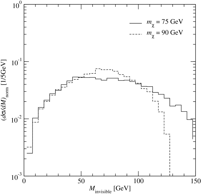
Figure 4: Missing invariant mass distributions for $e^{+}e^{-}\to\tilde{\chi}^{0}_{1}\tilde{\chi}^{0}_{1}\to\gamma\gamma\tilde{G}\tilde{G}$ at $\sqrt{s}=190$ GeV. The cases for the neutralino mass $m_{\chi}=75$ and 90 GeV are shown as a solid and dashed line, respectively, with the normalized cross section after kinematical cuts of (14).

3 Summary

In this paper, we have added new HELAS subroutines to calculate helicity amplitudes with massive spin-3/2 particles (massive gravitinos) to the HELAS library. They are coded in such a way that arbitrary amplitudes with external gravitinos can be generated automatically by MG, after slight modifications. All the codes have been tested carefully by making use of the gauge invariance of the helicity amplitudes.

Appendix A HELAS subroutines for spin-3/2 particles

In this appendix, we list the contents of all the new HELAS subroutines that are needed to evaluate processes based on the effective Lagrangian of (2) with external spin-3/2 gravitinos.

To begin with, in App. A.1 the subroutines to compute external lines for a massive spin-3/2 particle are presented. Next, in Apps. A.2 to A.5, we explain vertex subroutines listed in Table 1, which compute interactions of a gravitino with SM and SUSY particles. Finally, we briefly mention how we test our new subroutines in App. A.6.

A.1 Spin-3/2 wavefunction

A.1.1 IRXXXX

This subroutine computes the flowing-In Rarita-Schwinger (R-S) spin-3/2 wavefunction; namely $\psi^{\mu}_{u}(p,\lambda)$ and $\psi^{\mu}_{v}(p,\lambda)$, in terms of its four-momentum $p$ and helicity $\lambda$, and should be called as

$${\tt CALL\ IRXXXX(P,RMASS,NHEL,NSR\ ,\ RI)}.$$

The input P(0:3) is a real four-dimensional array which contains the four-momentum $p^{\mu}$ of the spin-3/2 particle, RMASS is its mass, NHEL (${\tt=\pm 3,\pm 1}$) specifies its helicity $\lambda$ in unit of 1/2, and NSR specifies whether the fermion is particle or anti-particle. If NSR = 1 the fermion is particle and the subroutine computes the wavefunction with the $u$-spinor. If NSR = -1 the fermion is anti-particle and the subroutine computes the wavefunction with the $v$-spinor. The output RI(18) is a complex 18-dimensional array, among which the first 16 components contain the wavefunction as

$${\tt RI(4\mu+i)=R(\mu+1,i)},$$ (15)

namely

$${\tt RI(\ 1)=R(1,1)},$$

$${\tt RI(\ 2)=R(1,2)},$$

$${\tt RI(\ 3)=R(1,3)},$$

$${\tt RI(\ 4)=R(1,4)},$$

$${\tt......}$$

$${\tt RI(16)=R(4,4)},$$

where

$${\tt R(\mu+1,i)}=\begin{cases}\psi^{\mu}_{u_{i}}(p,\lambda)&\text{for {\tt NSR = 1}},\\ \psi^{\mu}_{v_{i}}(p,\lambda)&\text{for {\tt NSR = -1}}.\end{cases}$$ (16)

Here, $i=1,2,3,4$ denotes each $u$- or $v$-spinor component. The last two of RI(18) contain the four-momentum along the fermion number flow,

$$({\tt RI(17)},\,{\tt RI(18)})={\tt NSR}\,({\tt P(0)}+i{\tt P(3)},\,{\tt P(1)}+i{\tt P(2)}).$$ (17)

Vertex	Inputs	Output	Subroutine
FRS	FRS	Amplitude	IORSXX, IROSXX
	RS	F	FSORXX, FSIRXX
	FR	S	HIORXX, HIROXX
FRV	FRV	Amplitude	IORVXX, IROVXX
	RV	F	FVORXX, FVIRXX
	FR	V	JIORXX, JIROXX
FRVS	FRVS	Amplitude	IORVSX, IROVSX
	RVS	F	FVSORX, FVSIRX
	FRS	V	JSIORX, JSIROX
	FRV	S	HVIORX, HVIROX
FRVV	FRVV	Amplitude	IORVVX, IROVVX
	RVV	F	FVVORX, FVVIRX
	FRV	V	JVIORX, JVIROX

Table 1: List of the new vertex subroutines in HELAS system.

When the four-momentum of the R-S fermion is given by

$$p^{\mu}=(E,\,|\vec{p}|\sin\theta\cos\phi,\,|\vec{p}|\sin\theta\sin\phi,\,|\vec{p}|\cos\theta),$$ (18)

its helicity states can be expressed as

$$\psi^{\mu}_{u}(p,+3/2) =\epsilon^{\mu}(p,+)\,u(p,+),$$

$$\psi^{\mu}_{u}(p,+1/2) =\sqrt{\frac{2}{3}}\,\epsilon^{\mu}(p,0)\,u(p,+)$$

$$\quad+\sqrt{\frac{1}{3}}\,\epsilon^{\mu}(p,+)\,u(p,-)\,e^{i\phi},$$

$$\psi^{\mu}_{u}(p,-1/2) =\sqrt{\frac{1}{3}}\,\epsilon^{\mu}(p,-)\,u(p,+)$$

$$\quad+\sqrt{\frac{2}{3}}\,\epsilon^{\mu}(p,0)\,u(p,-)\,e^{i\phi},$$

$$\psi^{\mu}_{u}(p,-3/2) =\epsilon^{\mu}(p,-)\,u(p,-)\,e^{i\phi},$$ (19)

by using the vector boson wavefunctions $\epsilon^{\mu}(p,\lambda)$ and the spinor wavefunctions $u(p,\lambda)$ that obey the relations

$$J_{-}\,\epsilon^{\mu}(p,\lambda) =\sqrt{2}\,\epsilon^{\mu}(p,\lambda-1),$$ (20)

$$J_{-}\,u(p,+) =e^{i\phi}\,u(p,-),$$ (21)

where $J_{-}=J_{x}-iJ_{y}$ is the $J_{z}$ lowering operator. The vector and spinor wavefunctions in the HELAS convention Hagiwara:1990dw satisfy above relations. Similarly, $\psi^{\mu}_{v}(p,\lambda)$ is given by the $v$-spinors and the conjugated vector wavefunctions. The above helicity states satisfy the irreducibility conditions and the Dirac equation,

$$\gamma_{\mu}\psi^{\mu}_{u}(p,\lambda)=0,\quad p_{\mu}\psi^{\mu}_{u}(p,\lambda)=0,$$ (22)

$$(\not\!p-m_{3/2})\psi^{\mu}_{u}(p,\lambda)=0,$$ (23)

and the completeness relation is

$$\sum_{\lambda=-3/2}^{+3/2}\psi^{\mu}_{u}(p,\lambda)\overline{\psi}^{\nu}_{u}(p,\lambda)=P^{\mu\nu}(p),$$ (24)

where

$$P^{\mu\nu}(p)=(\not\!p+m_{3/2})\Big{(}\Pi^{\mu\nu}(p)+\frac{1}{3}\Pi^{\mu\alpha}(p)\Pi^{\nu\beta}(p)\gamma_{\alpha}\gamma_{\beta}\Big{)}$$ (25)

with

$$\Pi^{\mu\nu}(p)=-g^{\mu\nu}+\frac{p^{\mu}p^{\nu}}{m_{3/2}^{2}}.$$ (26)

A.1.2 ORXXXX

This subroutine computes the flowing-Out R-S wavefunction; namely, $\overline{\psi}^{\mu}_{u}(p,\lambda)$ and $\overline{\psi}^{\mu}_{v}(p,\lambda)$, and should be called as

$${\tt CALL\ ORXXXX(P,RMASS,NHEL,NSR\ ,\ RO)}.$$

As in the subroutine IRXXXX, the output RO(18) is a complex 18-dimensional array, among which the first 16 components contain the wavefunction as

$${\tt RO(4\mu+i)=\bar{R}(\mu+1,i)},$$ (27)

where

$${\tt\bar{R}(\mu+1,i)}=\begin{cases}\overline{\psi}^{\mu}_{u_{i}}(p,\lambda)&\text{for {\tt NSR = 1}},\\ \overline{\psi}^{\mu}_{v_{i}}(p,\lambda)&\text{for {\tt NSR = -1}},\end{cases}$$ (28)

and the last two are the four-momentum

$$({\tt RO(17)},\,{\tt RO(18)})={\tt NSR}\,({\tt P(0)}+i{\tt P(3)},\,{\tt P(1)}+i{\tt P(2)}).$$ (29)

A.2 FRS vertex

The FRS vertices are obtained from the interaction Lagrangian among a fermion, a R-S fermion and a scalar boson:

$${\cal L}_{\tt FRS}=-i\overline{R}_{\mu}\gamma^{\nu}\gamma^{\mu}[{\tt GR(1)}P_{L}+{\tt GR(2)}P_{R}]f\,\partial_{\nu}S^{*}+{\rm h.c.}$$ (30)

with the notation $R^{\mu}=\psi^{\mu}_{u/v}$ and the chiral-projection operator $P_{R/L}=\frac{1}{2}(1\pm\gamma_{5})$. GR(1) and GR(2) are the relevant left and right coupling constants. For instance, in the case of the quark-gravitino-squark interaction, $q$-$\tilde{G}$-$\tilde{q}_{\alpha}$, those couplings are

$$\begin{cases}{\tt GR(1)}={\tt GFRSL(1)}={\tt GFRS}\\ {\tt GR(2)}={\tt GFRSL(2)}=0\end{cases} {\rm for}\ \alpha=L,$$ (31)

$$\begin{cases}{\tt GR(1)}={\tt GFRSR(1)}=0\\ {\tt GR(2)}={\tt GFRSR(2)}=-{\tt GFRS}\end{cases} {\rm for}\ \alpha=R,$$ (32)

where

$${\tt GFRS}=1/\sqrt{2}\,\overline{M}_{\rm Pl}.$$ (33)

A.2.1 IORSXX

This subroutine computes an amplitude of the FRS vertex from wavefunctions of a flowing-In fermion, a flowing-Out R-S fermion and a Scalar boson, and should be called as

CALL IORSXX(FI,RO,SC,GR , VERTEX).

The input FI(6) is a complex six-dimensional array which contains the wavefunction of the flowing-In Fermion and its four-momentum as

$$p^{\mu}=(\Re e{\tt FI(5)},\Re e{\tt FI(6)},\Im m{\tt FI(6)},\Im m{\tt FI(5)}).$$

The input RO(18) is a complex 18-dimensional array which consists of the wavefunction and the four-momentum of the flowing-Out R-S fermion; see the ORXXXX subroutine in App. A.1.2, while the input SC(3) is a complex three-dimensional array which contains the wavefunction of the Scalar boson, SC(1), and its four-momentum as

$$q^{\mu}=(\Re e{\tt SC(2)},\Re e{\tt SC(3)},\Im m{\tt SC(3)},\Im m{\tt SC(2)}).$$

The input GR(2) is the complex coupling constant, such as in (31) and (32) in units of GeV^-1. The output VERTEX is a complex number in units of GeV:

$${\tt VERTEX}=({\tt RO})_{\mu}{\tt SC(1)}\!\!\not\!q\gamma^{\mu}[{\tt GR(1)}P_{L}+{\tt GR(2)}P_{R}]({\tt FI}),$$ (34)

where we use the notations

$$({\tt FI}) =\begin{pmatrix}{\tt FI(1)}\\ {\tt FI(2)}\\ {\tt FI(3)}\\ {\tt FI(4)}\end{pmatrix},$$ (35)

$$({\tt RO})_{\mu} ={\tt(RO(4\mu+1),RO(4\mu+2),RO(4\mu+3),RO(4\mu+4))}.$$ (36)

A.2.2 IROSXX

This subroutine computes an amplitude of the FRS vertex from wavefunctions of a flowing-In R-S fermion, a flowing-Out fermion and a Scalar boson, and should be called as

CALL IROSXX(RI,FO,SC,GR , VERTEX).

The input RI(18) is a complex 18-dimensional array which consists of the wavefunction and the four-momentum of the flowing-In R-S fermion; see the IRXXXX subroutine in App. A.1.1, while the input FO(6) is a complex six-dimensional array which contains the wavefunction of the flowing-Out Fermion and its four-momentum as

$$p^{\mu}=(\Re e{\tt FO(5)},\Re e{\tt FO(6)},\Im m{\tt FO(6)},\Im m{\tt FO(5)}).$$

The output VERTEX is a complex number:

$${\tt VERTEX}=-{\tt(FO)}{\tt SC(1)}[{\tt GR(1)}^{*}P_{R}+{\tt GR(2)^{*}}P_{L}]\gamma^{\mu}\!\!\not\!q({\tt RI})_{\mu},$$ (37)

where $q^{\mu}$ is the momentum of the scalar boson and we use the notations

$$({\tt RI})_{\mu} =\begin{pmatrix}{\tt RI(4\mu+1)}\\ {\tt RI(4\mu+2)}\\ {\tt RI(4\mu+3)}\\ {\tt RI(4\mu+4)}\end{pmatrix},$$ (38)

$${\tt(FO)} ={\tt(FO(1),FO(2),FO(3),FO(4)}).$$ (39)

A.2.3 FSORXX

This subroutine computes an off-shell Fermion wavefunction made from the interaction of a Scalar boson and a flowing-Out R-S fermion by the FRS vertex, and should be called as

CALL FSORXX(RO,SC,GR,FMASS,FWIDTH , FSOR),

where FMASS and FWIDTH are the mass and the width of the fermion, $m_{F}$ and $\Gamma_{F}$. The output FSOR(6) gives the off-shell fermion wavefunction multiplied by the fermion propagator and its four-momentum, which is expressed as a complex six-dimensional array:

$${\tt(FSOR)}=({\tt RO})_{\mu}{\tt SC(1)}\!\!\not\!q\gamma^{\mu}[i{\tt GR(1)}P_{L}+i{\tt GR(2)}P_{R}]\\ \times\frac{i(\not\!p+m_{F})}{p^{2}-m_{F}^{2}+im_{F}\Gamma_{F}},$$ (40)

and

$${\tt FSOR(5)} ={\tt RO(17)+SC(2)},$$ (41)

$${\tt FSOR(6)} ={\tt RO(18)+SC(3)}.$$ (42)

Here we use the notation

$$({\tt FSOR})=({\tt FSOR(1),FSOR(2),FSOR(3),FSOR(4)}),$$ (43)

and $p$ is the momentum of the off-shell fermion given in (41) and (42) as

$$p^{\mu}=(\Re e{\tt FSOR(5)},\Re e{\tt FSOR(6)},\Im m{\tt FSOR(6)},\Im m{\tt FSOR(5)}).$$

A.2.4 FSIRXX

The subroutine computes an off-shell Fermion wavefunction made from the interaction of a Scalar boson and a flowing-In R-S fermion by the FRS vertex, and should be called as

CALL FSIRXX(RI,SC,GR,FMASS,FWIDTH , FSIR).

The output FSIR(6) is a complex six-dimensional array:

$${\tt(FSIR)}=-\frac{i(\not\!p+m_{F})}{p^{2}-m_{F}^{2}+im_{F}\Gamma_{F}}\,{\tt SC(1)}\\ \times[i{\tt GR(1)}^{*}P_{R}+i{\tt GR(2)}^{*}P_{L}]\gamma^{\mu}\!\!\not\!q\,({\tt RI})_{\mu},$$ (44)

and

$${\tt FSIR(5)} ={\tt RI(17)-SC(2)},$$ (45)

$${\tt FSIR(6)} ={\tt RI(18)-SC(3)}.$$ (46)

Here we use the notation

$$({\tt FSIR})=\begin{pmatrix}{\tt FSIR(1)}\\ {\tt FSIR(2)}\\ {\tt FSIR(3)}\\ {\tt FSIR(4)}\end{pmatrix},$$ (47)

and the momentum $p$ is

$$p^{\mu}=(\Re e{\tt FSIR(5)},\Re e{\tt FSIR(6)},\Im m{\tt FSIR(6)},\Im m{\tt FSIR(5)}).$$

A.2.5 HIORXX

This subroutine computes an off-shell scalar current H made from the interaction of a flowing-In fermion and a flowing-Out R-S fermion by the FRS vertex, and should be called as

CALL HIORXX(FI,RO,GR,SMASS,SWIDTH , HIOR),

where SMASS and SWIDTH are the mass and the width of the scalar boson, $m_{S}$ and $\Gamma_{S}$. The output HIOR(3) gives the off-shell scalar current multiplied by the scalar boson propagator and its four-momentum, which is expressed as a complex three-dimensional array:

$${\tt HIOR(1)}=-\frac{i}{q^{2}-m_{S}^{2}+im_{S}\Gamma_{S}}\\ \times({\tt RO})_{\mu}\!\!\not\!q\gamma^{\mu}[i{\tt GR(1)}P_{L}+i{\tt GR(2)}P_{R}]({\tt FI}),$$ (48)

and

$${\tt HIOR(2)} ={\tt-FI(5)+RO(17)},$$ (49)

$${\tt HIOR(3)} ={\tt-FI(6)+RO(18)}.$$ (50)

The momentum $q$ is

$$q^{\mu}=(\Re e{\tt HIOR(2)},\Re e{\tt HIOR(3)},\Im m{\tt HIOR(3)},\Im m{\tt HIOR(2)}).$$

A.2.6 HIROXX

This subroutine computes an off-shell scalar current H made from the interaction of a flowing-In R-S fermion and a flowing-Out fermion by the FRS vertex, and should be called as

CALL HIROXX(RI,FO,GR,SMASS,SWIDTH , HIRO).

The output HIRO(3) is a complex three-dimensional array:

$${\tt HIRO(1)}=\frac{i}{q^{2}-m_{S}^{2}+im_{S}\Gamma_{S}}\\ \times({\tt FO})[i{\tt GR(1)}^{*}P_{R}+i{\tt GR(2)}^{*}P_{L}]\gamma^{\mu}\!\!\not\!q({\tt RI})_{\mu},$$ (51)

and

$${\tt HIRO(2)} ={\tt-RI(17)+FO(5)},$$ (52)

$${\tt HIRO(3)} ={\tt-RI(18)+FO(6)}.$$ (53)

The momentum $q$ is

$$q^{\mu}=(\Re e{\tt HIRO(2)},\Re e{\tt HIRO(3)},\Im m{\tt HIRO(3)},\Im m{\tt HIRO(2)}).$$

Before turning to the FRV vertex, it should be noticed here that the conventional factors of $i$ in the vertices and those in the propagators are both included in the off-shell wavefunctions, such as (40) above, according to the HELAS convention. The HELAS amplitude, obtained by the vertices, such as (34), gives the contribution to the $T$ matrix element without the factor of $i$. See more details in the HELAS manual Hagiwara:1990dw .

A.3 FRV vertex

The FRV vertices are obtained from the interaction Lagrangian among a fermion, a R-S fermion and a vector boson:

$${\cal L}_{\tt FRV}=-i\overline{R}_{\mu}[\gamma^{\nu},\gamma^{\rho}]\gamma^{\mu}[{\tt GR(1)}P_{L}+{\tt GR(2)}P_{R}]f\,\partial_{\nu}V^{*}_{\rho}+{\rm h.c.}$$ (54)

We note that, although both a gravitino and a gaugino are Majorana in most cases, the Hermitian conjugate term is necessary for MG; practically, either the first or second term is used in calculations of amplitudes. The corresponding coupling constant to the effective Lagrangian of (2) is

$${\tt GR(1)}={\tt GR(2)}={\tt GFRV}=1/4\overline{M}_{\rm Pl}.$$ (55)

A.3.1 IORVXX

This subroutine computes an amplitude of the FRV vertex from wavefunctions of a flowing-In fermion, a flowing-Out R-S fermion and a Vector boson, and should be called as

CALL IORVXX(FI,RO,VC,GR , VERTEX).

The input VC(6) is a complex six-dimensional array which contains the Vector boson wavefunction and its momentum as

$$q^{\mu}=(\Re e{\tt VC(5)},\Re e{\tt VC(6)},\Im m{\tt VC(6)},\Im m{\tt VC(5)}).$$

The input GR is the coupling constant in (55). The output VERTEX is a complex number:

$${\tt VERTEX}=({\tt RO})_{\mu}[\not\!q,\not\!V]\gamma^{\mu}[{\tt GR(1)}P_{L}+{\tt GR(2)}P_{R}]({\tt FI}),$$ (56)

where we use the notation

$$V^{\mu}={\tt VC}(\mu+1).$$ (57)

A.3.2 IROVXX

This subroutine computes an amplitude of the FRV vertex from wavefunctions of a flowing-In R-S fermion, a flowing-Out fermion and a Vector boson, and should be called as

CALL IROVXX(RI,FO,VC,GR , VERTEX).

The output VERTEX is

$${\tt VERTEX}=-({\tt FO})[{\tt GR(1)}^{*}P_{R}+{\tt GR(2)}^{*}P_{L}]\gamma^{\mu}[\not\!V,\not\!q]({\tt RI})_{\mu}.$$ (58)

A.3.3 FVORXX

This subroutine computes an off-shell Fermion wavefunction made from the interaction of a Vector boson and a flowing-Out R-S fermion by the FRV vertex, and should be called as

CALL FVORXX(RO,VC,GR,FMASS,FWIDTH , FVOR).

What we compute here is

$${\tt(FVOR)}=({\tt RO})_{\mu}[\not\!q,\not\!V]\gamma^{\mu}[i{\tt GR(1)}P_{L}+i{\tt GR(2)}P_{R}]\\ \times\frac{i(\not\!p+m_{F})}{p^{2}-m_{F}^{2}+im_{F}\Gamma_{F}},$$ (59)

and

$${\tt FVOR(5)} ={\tt RO(17)+VC(5)},$$ (60)

$${\tt FVOR(6)} ={\tt RO(18)+VC(6)},$$ (61)

where we use the notation

$$({\tt FVOR})= ({\tt FVOR(1),FVOR(2),FVOR(3),FVOR(4)}),$$ (62)

and the momentum $p$ is

$$p^{\mu}=(\Re e{\tt FVOR(5)},\Re e{\tt FVOR(6)},\Im m{\tt FVOR(6)},\Im m{\tt FVOR(5)}).$$

A.3.4 FVIRXX

This subroutine computes an off-shell Fermion wavefunction made from the interaction of a Vector boson and a flowing-In R-S fermion by the FRV vertex, and should be called as

CALL FVIRXX(RI,VC,GR,FMASS,FWIDTH , FVIR).

What we compute here is

$${\tt(FVIR)}=-\frac{i(\not\!p+m_{F})}{p^{2}-m_{F}^{2}+im_{F}\Gamma_{F}}\\ \times[i{\tt GR(1)}^{*}P_{R}+i{\tt GR(2)}^{*}P_{L}]\gamma^{\mu}[\not\!V,\not\!q]({\tt RI})_{\mu},$$ (63)

and

$${\tt FVIR(5)} ={\tt RI(17)-VC(5)},$$ (64)

$${\tt FVIR(6)} ={\tt RI(18)-VC(6)},$$ (65)

where we use the notation

$$({\tt FVIR})= \begin{pmatrix}{\tt FVIR(1)}\\ {\tt FVIR(2)}\\ {\tt FVIR(3)}\\ {\tt FVIR(4)}\end{pmatrix},$$ (66)

and the momentum $p$ is

$$p^{\mu}=(\Re e{\tt FVIR(5)},\Re e{\tt FVIR(6)},\Im m{\tt FVIR(6)},\Im m{\tt FVIR(5)}).$$

A.3.5 JIORXX

This subroutine computes an off-shell vector current J made from the interaction of a flowing-In fermion and a flowing-Out R-S fermion by the FRV vertex, and should be called as

CALL JIORXX(FI,RO,GR,VMASS,VWIDTH , JIOR).

The input VMASS and VWIDTH are the mass and the width of the vector boson, $m_{V}$ and $\Gamma_{V}$. The output JIOR(6) gives the off-shell vector current multiplied by the vector boson propagator and its four-momentum, which is expressed as a complex six-dimensional array:

$${\tt JIOR(\nu+1)}=-\frac{i}{q^{2}-m_{V}^{2}+im_{V}\Gamma_{V}}\left(-g^{\rho\nu}+\frac{q^{\rho}q^{\nu}}{m_{V}^{2}}\right)\\ \times({\tt RO})_{\mu}[\not\!q,\gamma_{\rho}]\gamma^{\mu}[i{\tt GR(1)}P_{L}+i{\tt GR(2)}P_{R}]({\tt FI})$$ (67)

for the massive vector boson, or

$${\tt JIOR(\nu+1)}=-\frac{-i}{q^{2}}\\ \times({\tt RO})_{\mu}[\not\!q,\gamma^{\nu}]\gamma^{\mu}[i{\tt GR(1)}P_{L}+i{\tt GR(2)}P_{R}]({\tt FI})$$ (68)

for the massless vector boson, and

$${\tt JIOR(5)} ={\tt-FI(5)+RO(17)},$$ (69)

$${\tt JIOR(6)} ={\tt-FI(6)+RO(18)}.$$ (70)

Here, $q$ is the momentum of the off-shell vector boson,

$$q^{\mu}= ({\tt\Re eJIOR(5),\Re eJIOR(6),\Im mJIOR(6),\Im mJIOR(5)}).$$

Note that we use the unitary gauge for the massive vector boson propagator and the Feynman gauge for the massless one, according to the HELAS convention Hagiwara:1990dw .

A.3.6 JIROXX

This subroutine computes an off-shell vector current J made from the interaction of a flowing-In R-S fermion and a flowing-Out fermion by the FRV vertex, and should be called as

CALL JIROXX(RI,FO,GR,VMASS,VWIDTH , JIRO).

The output JIRO(6) is

$${\tt JIRO(\nu+1)}=\frac{i}{q^{2}-m_{V}^{2}+im_{V}\Gamma_{V}}\left(-g^{\rho\nu}+\frac{q^{\rho}q^{\nu}}{m_{V}^{2}}\right)\\ \times({\tt FO})[i{\tt GR(1)}^{*}P_{R}+i{\tt GR(2)}^{*}P_{L}]\gamma^{\mu}[\gamma_{\rho},\not\!q]({\tt RI})_{\mu}$$ (71)

for the massive vector boson, or

$${\tt JIRO(\nu+1)}=\frac{-i}{q^{2}}\\ \times({\tt FO})[i{\tt GR(1)}^{*}P_{R}+i{\tt GR(2)}^{*}P_{L}]\gamma^{\mu}[\gamma^{\nu},\not\!q]({\tt RI})_{\mu}$$ (72)

for the massless vector boson, and

$${\tt JIRO(5)} ={\tt-RI(17)+FO(5)},$$ (73)

$${\tt JIRO(6)} ={\tt-RI(18)+FO(6)}.$$ (74)

Here the momentum $q$ is

$$q^{\mu}=({\tt\Re eJIRO(5),\Re eJIRO(6),\Im mJIRO(6),\Im mJIRO(5)}).$$

A.4 FRVS vertex

The FRVS vertices are obtained from the interaction Lagrangian among a fermion, a R-S fermion, a vector boson and a scalar boson:

$${\cal L}_{\tt FRVS}=\overline{R}_{\mu}\gamma^{\nu}\gamma^{\mu}[{\tt GR(1)}P_{L}+{\tt GR(2)}P_{R}]f\,V_{\nu}^{*}S^{*}+{\rm h.c.}$$ (75)

The coupling constant GR is the product of the FRS coupling constant and the gauge coupling constant of the involving gauge boson. For instance, in the case of the quark-gravitino-gluon-squark interaction, $q$-$\tilde{G}$-$g$-$\tilde{q}_{L}$, those couplings are

$$\begin{cases}{\tt GR(1)}={\tt GFRGSL(1)}={\tt GFRSL(1)*GG(1)},\\ {\tt GR(2)}={\tt GFRGSL(2)}={\tt GFRSL(2)*GG(2)},\end{cases}$$ (76)

where GFRSL is defined in (31) and GG is the strong coupling constant

$${\tt GG(1)}={\tt GG(2)}=-g_{s}=-{\tt G}.$$ (77)

The sign of the coupling constant is fixed by the HELAS convention Hagiwara:1990dw .

A.4.1 IORVSX

This subroutine computes an amplitude of the FRVS vertex from a flowing-In fermion, a flowing-Out R-S fermion, a Vector boson and a Scalar boson, and should be called as

CALL IORVSX(FI,RO,VC,SC,GR , VERTEX).

The output VERTEX gives a complex number:

$${\tt VERTEX}=({\tt RO})_{\mu}{\tt SC(1)}\!\not\!V\gamma^{\mu}[{\tt GR(1)}P_{L}+{\tt GR(2)}P_{R}]({\tt FI}).$$ (78)

A.4.2 IROVSX

This subroutine computes an amplitude of the FRVS vertex from a flowing-In R-S fermion, a flowing-Out fermion, a Vector boson and a Scalar boson, and should be called as

CALL IROVSX(RI,FO,VC,SC,GR , VERTEX).

The output VERTEX gives a complex number:

$${\tt VERTEX}=({\tt FO})\,{\tt SC(1)}[{\tt GR(1)}^{*}P_{R}+{\tt GR(2)}^{*}P_{L}]\gamma^{\mu}\!\not\!V({\tt RI})_{\mu}.$$ (79)

A.4.3 FVSORX

This subroutine computes an off-shell Fermion wavefunction made from the interaction of a Vector boson, a Scalar boson and a flowing-Out R-S fermion by the FRVS vertex, and should be called as

$${\tt CALL\ FVSORX(RO,VC,SC,GR,FMASS,FWIDTH\ ,\ FVSOR)}.$$

The output FVSOR is a complex six-dimensional array:

$${\tt(FVSOR)}=({\tt RO})_{\mu}{\tt SC(1)}\!\not\!V\gamma^{\mu}[i{\tt GR(1)}P_{L}+i{\tt GR(2)}P_{R}]\\ \times\frac{i(\not\!p+m_{F})}{p^{2}-m_{F}^{2}+im_{F}\Gamma_{F}}$$ (80)

for the first four components of FVSOR(6), and

$${\tt FVSOR(5)} ={\tt RO(17)+VC(5)+SC(2)},$$ (81)

$${\tt FVSOR(6)} ={\tt RO(18)+VC(6)+SC(3)},$$ (82)

for the momentum $p$.

A.4.4 FVSIRX

This subroutine computes an off-shell Fermion wavefunction made from the interaction of a Vector boson, a Scalar boson and a flowing-In R-S fermion by the FRVS vertex, and should be called as

$${\tt CALL\ FVSIRX(RI,VC,SC,GR,FMASS,FWIDTH\ ,\ FVSIR)}.$$

The output FVSIR is a complex six-dimensional array:

$${\tt(FVSIR)}=\frac{i(\not\!p+m_{F})}{p^{2}-m_{F}^{2}+im_{F}\Gamma_{F}}\,{\tt SC(1)}\\ \times[i{\tt GR(1)}^{*}P_{R}+i{\tt GR(2)}^{*}P_{L}]\gamma^{\mu}\!\not\!V({\tt RI})_{\mu}$$ (83)

for the first four components of FVSIR(6), and

$${\tt FVSIR(5)} ={\tt RI(17)-VC(5)-SC(2)},$$ (84)

$${\tt FVSIR(6)} ={\tt RI(18)-VC(6)-SC(3)},$$ (85)

for the momentum $p$.

A.4.5 JSIORX

This subroutine computes an off-shell vector current J made from the interaction of a Scalar boson, a flowing-In fermion and a flowing-Out R-S fermion by the FRVS vertex, and should be called as

CALL JSIORX(FI,RO,SC,GR,VMASS,VWIDTH , JSIOR).

What we compute here is

$${\tt JSIOR(\nu+1)}=\frac{i}{q^{2}-m_{V}^{2}+im_{V}\Gamma_{V}}\left(-g^{\rho\nu}+\frac{q^{\rho}q^{\nu}}{m_{V}^{2}}\right)\\ \times({\tt RO})_{\mu}{\tt SC(1)}\,\gamma_{\rho}\gamma^{\mu}[i{\tt GR(1)}P_{L}+i{\tt GR(2)}P_{R}]({\tt FI})$$ (86)

for the massive vector boson, or

$${\tt JSIOR(\nu+1)}=\frac{-i}{q^{2}}\\ \times({\tt RO})_{\mu}{\tt SC(1)}\,\gamma^{\nu}\gamma^{\mu}[i{\tt GR(1)}P_{L}+i{\tt GR(2)}P_{R}]({\tt FI})$$ (87)

for the massless vector boson, and

$${\tt JSIOR(5)} ={\tt-FI(5)+RO(17)+SC(2)},$$ (88)

$${\tt JSIOR(6)} ={\tt-FI(6)+RO(18)+SC(3)},$$ (89)

for the momentum $q$.

A.4.6 JSIROX

This subroutine computes an off-shell vector current J made from the interaction of a Scalar boson, a flowing-In R-S fermion and a flowing-Out fermion by the FRVS vertex, and should be called as

CALL JSIROX(RI,FO,SC,GR,VMASS,VWIDTH , JSIRO).

What we compute here is

$${\tt JSIRO(\nu+1)}=\frac{i}{q^{2}-m_{V}^{2}+im_{V}\Gamma_{V}}\left(-g^{\rho\nu}+\frac{q^{\rho}q^{\nu}}{m_{V}^{2}}\right)\\ \times({\tt FO})\,{\tt SC(1)}[i{\tt GR(1)}^{*}P_{R}+i{\tt GR(2)}^{*}P_{L}]\gamma^{\mu}\gamma_{\rho}({\tt RI})_{\mu}$$ (90)

for the massive vector boson, or

$${\tt JSIRO(\nu+1)}=\frac{-i}{q^{2}}\\ \times({\tt FO})\,{\tt SC(1)}[i{\tt GR(1)}^{*}P_{R}+i{\tt GR(2)}^{*}P_{L}]\gamma^{\mu}\gamma^{\nu}({\tt RI})_{\mu}$$ (91)

for the massless vector boson, and

$${\tt JSIRO(5)} ={\tt-RI(17)+FO(5)+SC(2)},$$ (92)

$${\tt JSIRO(6)} ={\tt-RI(18)+FO(6)+SC(3)},$$ (93)

for the momentum $q$.

A.4.7 HVIORX

This subroutine computes an off-shell scalar current H made from the interaction of a Vector boson, a flowing-In fermion and a flowing-Out R-S fermion by the FRVS vertex, and should be called as

$${\tt CALL\ HVIORX(FI,RO,VC,GR,SMASS,SWIDTH\ ,\ HVIOR)}.$$

What we compute here is

$${\tt HVIOR(1)}=\frac{i}{q^{2}-m_{S}^{2}+im_{S}\Gamma_{S}}\\ \times({\tt RO})_{\mu}\!\not\!V\gamma^{\mu}[i{\tt GR(1)}P_{L}+i{\tt GR(2)}P_{R}]({\tt FI}),$$ (94)

and

$${\tt HVIOR(2)} ={\tt-FI(5)+RO(17)+VC(5)},$$ (95)

$${\tt HVIOR(3)} ={\tt-FI(6)+RO(18)+VC(6)},$$ (96)

for the momentum $q$.

A.4.8 HVIROX

This subroutine computes an off-shell scalar current H made from the interaction of a Vector boson, a flowing-In R-S fermion and a flowing-Out fermion by the FRVS vertex, and should be called as

$${\tt CALL\ HVIROX(RI,FO,VC,GR,SMASS,SWIDTH\ ,\ HVIRO)}.$$

What we compute here is

$${\tt HVIRO(1)}=\frac{i}{q^{2}-m_{S}^{2}+im_{S}\Gamma_{S}}\\ \times({\tt FO})[i{\tt GR(1)}^{*}P_{R}+i{\tt GR(2)}^{*}P_{L}]\gamma^{\mu}\!\not\!V({\tt RI})_{\mu},$$ (97)

and

$${\tt HVIRO(2)} ={\tt-RI(17)+FO(5)+VC(5)},$$ (98)

$${\tt HVIRO(3)} ={\tt-RI(18)+FO(6)+VC(6)},$$ (99)

for the momentum $q$.

A.5 FRVV vertex

The FRVV vertices are obtained from the interaction Lagrangian among a fermion, a R-S fermion and two vector bosons:

$${\cal L}_{\tt FRVV}=if^{abc}\overline{R}_{\mu}[\gamma^{\nu},\gamma^{\rho}]\gamma^{\mu}[{\tt GR(1)}P_{L}+{\tt GR(2)}P_{R}]f^{a}\,V_{\nu}^{b}V_{\rho}^{c}\\ +{\rm h.c.}$$ (100)

with the structure constant $f^{abc}$, which can be handled by the MG automatically. The coupling constant GR is the product of the FRV coupling constant and the gauge coupling constant of the involving gauge boson as in the FRVS coupling; see (76).

A.5.1 IORVVX

This subroutine computes an amplitude of the FRVV vertex from a flowing-In fermion, a flowing-Out R-S fermion and two Vector bosons, and should be called as

CALL IORVVX(FI,RO,VA,VB,GR , VERTEX).

What we compute here is

$${\tt VERTEX}=({\tt RO})_{\mu}[\not\!V^{a},\not\!V^{b}]\gamma^{\mu}[{\tt GR(1)}P_{L}+{\tt GR(2)}P_{R}]({\tt FI}),$$ (101)

where we use the notations

$$V^{a,\mu} ={\tt VA}(\mu+1),$$ (102)

$$V^{b,\mu} ={\tt VB}(\mu+1).$$ (103)

A.5.2 IROVVX

This subroutine computes an amplitude of the FRVV vertex from a flowing-In R-S fermion, a flowing-Out fermion and two Vector bosons, and should be called as

CALL IROVVX(RI,FO,VA,VB,GR , VERTEX).

What we compute here is

$${\tt VERTEX}=({\tt FO})[{\tt GR(1)}^{*}P_{R}+{\tt GR(2)}^{*}P_{L}]\gamma^{\mu}[\not\!V^{a},\not\!V^{b}]({\tt RI})_{\mu}.$$ (104)

A.5.3 FVVORX

This subroutine computes an off-shell Fermion wavefunction made from the interaction of two Vector bosons and a flowing-Out R-S fermion by the FRVV vertex, and should be called as

$${\tt CALL\ FVVORX(RO,VA,VB,GR,FMASS,FWIDTH\ ,\ FVVOR)}.$$

What we compute here is

$${\tt(FVVOR)}=({\tt RO})_{\mu}[\not\!V^{a},\not\!V^{b}]\gamma^{\mu}[i{\tt GR(1)}P_{L}+i{\tt GR(2)}P_{R}]\\ \times\frac{i(\not\!p+m_{F})}{p^{2}-m_{F}^{2}+im_{F}\Gamma_{F}},$$ (105)

and

$${\tt FVVOR(5)} ={\tt RO(17)+VA(5)+VB(5)},$$ (106)

$${\tt FVVOR(6)} ={\tt RO(18)+VA(6)+VB(6)}.$$ (107)

A.5.4 FVVIRX

This subroutine computes an off-shell Fermion wavefunction made from the interaction of two Vector bosons and a flowing-In R-S fermion by the FRVV vertex, and should be called as

$${\tt CALL\ FVVIRX(RI,VA,VB,GR,FMASS,FWIDTH\ ,\ FVVIR)}.$$

What we compute here is

$${\tt(FVVIR)}=\frac{i(\not\!p+m_{F})}{p^{2}-m_{F}^{2}+im_{F}\Gamma_{F}}\\ \times[i{\tt GR(1)}^{*}P_{R}+i{\tt GR(2)}^{*}P_{L}]\gamma^{\mu}[\not\!V^{a},\not\!V^{b}]({\tt RI})_{\mu},$$ (108)

and

$${\tt FVVIR(5)} ={\tt RI(17)-VA(5)-VB(5)},$$ (109)

$${\tt FVVIR(6)} ={\tt RI(18)-VA(6)-VB(6)}.$$ (110)

A.5.5 JVIORX

This subroutine computes an off-shell vector current J made from the interaction of a Vector boson, a flowing-In fermion and a flowing-Out R-S fermion by the FRVV vertex, and should be called as

CALL JVIORX(FI,RO,VC,GR,VMASS,VWIDTH , JVIOR).

What we compute here is

$${\tt JVIOR(\nu+1)}=\frac{i}{q^{2}-m_{V}^{2}+im_{V}\Gamma_{V}}\left(-g^{\rho\nu}+\frac{q^{\rho}q^{\nu}}{m_{V}^{2}}\right)\\ \times({\tt RO})_{\mu}[\gamma_{\rho},\not\!V]\gamma^{\mu}[i{\tt GR(1)}P_{L}+i{\tt GR(2)}P_{R}]({\tt FI})$$ (111)

for the massive vector boson, or

$${\tt JVIOR(\nu+1)}=\frac{-i}{q^{2}}\\ \times({\tt RO})_{\mu}[\gamma^{\nu},\not\!V]\gamma^{\mu}[i{\tt GR(1)}P_{L}+i{\tt GR(2)}P_{R}]({\tt FI})$$ (112)

for the massless vector boson, and

$${\tt JVIOR(5)} ={\tt-FI(5)+RO(17)+VC(5)},$$ (113)

$${\tt JVIOR(6)} ={\tt-FI(6)+RO(18)+VC(6)}.$$ (114)

A.5.6 JVIROX

This subroutine computes an off-shell vector current J made from the interaction of a Vector boson, a flowing-In R-S fermion and a flowing-Out fermion by the FRVV vertex, and should be called as

CALL JVIROX(RI,FO,VC,GR,VMASS,VWIDTH , JVIRO).

What we compute here is

$${\tt JVIRO(\nu+1)}=\frac{i}{q^{2}-m_{V}^{2}+im_{V}\Gamma_{V}}\left(-g^{\rho\nu}+\frac{q^{\rho}q^{\nu}}{m_{V}^{2}}\right)\\ \times({\tt FO})[i{\tt GR(1)}^{*}P_{R}+i{\tt GR(2)}^{*}P_{L}]\gamma^{\mu}[\gamma_{\rho},\not\!V]({\tt RI})_{\mu}$$ (115)

for the massive vector boson, or

$${\tt JVIRO(\nu+1)}=\frac{-i}{q^{2}}\\ \times({\tt FO})[i{\tt GR(1)}^{*}P_{R}+i{\tt GR(2)}^{*}P_{L}]\gamma^{\mu}[\gamma^{\nu},\not\!V]({\tt RI})_{\mu}$$ (116)

for the massless vector boson, and

$${\tt JVIRO(5)} ={\tt-RI(17)+FO(5)+VC(5)},$$ (117)

$${\tt JVIRO(6)} ={\tt-RI(18)+FO(6)+VC(6)}.$$ (118)

A.6 Checking for the new HELAS subroutines

The new HELAS subroutines are tested by using the gauge invariance of the helicity amplitudes. In particular, we use the following processes;

$$qg\to\tilde{q}\tilde{G} {\rm for}\ {\tt IORSXX},{\tt IROSXX},{\tt FSORXX},{\tt FSIRXX},$$

$${\tt HIORXX},{\tt HIROXX},{\tt IORVSX},{\tt IROVSX},$$

$$gg\to\tilde{g}\tilde{G} {\rm for}\ {\tt IORVXX},{\tt IROVXX},{\tt FVORXX},{\tt FVIRXX},$$

$${\tt JIORXX},{\tt JIROXX},{\tt IORVVX},{\tt IROVVX},$$

$$qg\to\tilde{q}\tilde{G}g {\rm for}\ {\tt FVSORX},{\tt FVSIRX},{\tt JSIORX},{\tt JSIROX},$$

$${\tt HVIORX},{\tt HVIROX},$$

$$gg\to\tilde{g}\tilde{G}g {\rm for}\ {\tt FVVORX},{\tt FVVIRX},{\tt JVIORX},{\tt JVIROX}.$$

More explicitly, we express the helicity amplitudes of the above processes as

$${\cal M}_{\lambda_{\tilde{G}}\lambda_{g}}=\bar{\psi}_{\mu}(p_{\tilde{G}},\lambda_{\tilde{G}})\,T^{\mu\nu}\epsilon_{\nu}(p_{g},\lambda_{g})$$ (119)

or

$${\cal M}_{\lambda_{\tilde{G}}\lambda_{g}}=T^{\mu\nu}\,\psi_{\mu}(p_{\tilde{G}},\lambda_{\tilde{G}})\,\epsilon_{\nu}(p_{g},\lambda_{g})$$ (120)

with an external spin-3/2 and a gluon wavefunction. The identity for the $SU(3)$ gauge invariance

$${p_{g}}_{\nu}\,T^{\mu\nu}=0$$ (121)

tests all the above subroutines thoroughly. We also test the agreement of the helicity-summed squared amplitudes at arbitrary Lorentz frames.

Appendix B Implementation of spin-3/2 gravitinos into MadGraph

3-point couplings							GR
FRS		q	gro	ql			GFRSL
		q	gro	qr			GFRSR
FRV		go	gro	g			GFRV
4-point couplings							GR
FRVS		q	gro	g	ql		GFRGSL	= GFRSL*GG
		q	gro	g	qr		GFRGSR	= GFRSR*GG
FRVV		go	gro	g	g		GGORGG	= GFRV*G

Table 2: List of the coupling constants for each gravitino vertex involving SUSY QCD particles. All the particles and the coupling constants are written in the MG notation. gro stands for a massive gravitino, q represents a light quark, and ql/qr is a left/right-handed squark. g and go are a gluon and a gluino, respectively. GR is a non-renormalizable coupling constant defined in each subroutine in App. A.

In this appendix, we describe how we implement spin-3/2 gravitinos and their interactions into MG.

First, using the default mssm model in MG/ME v4 Alwall:2007st , we make our new model directory, mssm_gravitino, including a massive gravitino (particles.dat) and its interactions with SM and SUSY particles (interactions.dat and couplings.f); we show the coupling constants for each gravitino vertex involving SUSY QCD particles in Table 2 as examples. Then we add all the new HELAS subroutines for spin-3/2 gravitinos to the HELAS library in MG. Since the present MG does not handle spin-3/2 particles, we further modify the codes in MG to tell it how to generate the FRS, FRV, FRVS and FRVV type of vertices and helicity amplitudes, and how to deal with the helicity of external spin-3/2 particles.

References

- (1) See, e.g., G. F. Giudice and R. Rattazzi, Phys. Rept. 322 (1999) 419.
- (2) W. Kilian, T. Ohl and J. Reuter, arXiv:0708.4233 [hep-ph].
- (3) K. Hagiwara, H. Murayama and I. Watanabe, Nucl. Phys. B 367 (1991) 257; H. Murayama, I. Watanabe and K. Hagiwara, KEK-Report 91-11, 1992.
- (4) T. Stelzer and W. F. Long, Comput. Phys. Commun. 81 (1994) 357.
- (5) F. Maltoni and T. Stelzer, JHEP 0302 (2003) 027.
- (6) J. Alwall, P. Demin, S. de Visscher, R. Frederix, M. Herquet, F .Maltoni, T. Plehn, D. Rainwaterd and T. Stelzer, JHEP 0709 (2007) 028.
- (7) J. Wess and J. Bagger, Princeton, USA: Univ. Pr. (1992) 259 p.
- (8) T. Moroi, arXiv:hep-ph/9503210.
- (9) M. Bolz, A. Brandenburg and W. Buchmuller, Nucl. Phys. B 606 (2001) 518 [Erratum-ibid. B 790 (2008) 336].
- (10) W. Buchmuller, K. Hamaguchi, M. Ratz and T. Yanagida, Phys. Lett. B 588 (2004) 90.
- (11) S. Ambrosanio, G. L. Kane, G. D. Kribs, S. P. Martin and S. Mrenna, Phys. Rev. D 54 (1996) 5395.
- (12) G. C. Cho, K. Hagiwara, J. Kanzaki, T. Plehn, D. Rainwater and T. Stelzer, Phys. Rev. D 73 (2006) 054002.