A Testable Solution of the Cosmological Constant and Coincidence Problems

Abstract

We present a new solution to the cosmological constant (CC) and coincidence problems in which the observed value of the CC, $\Lambda$, is linked to other observable properties of the universe. This is achieved by promoting the CC from a parameter which must to specified, to a field which can take many possible values. The observed value of $\Lambda\approx(9.3\,{\rm Gyrs})^{-2}$ ($\approx 10^{-120}$ in Planck units) is determined by a new constraint equation which follows from the application of a causally restricted variation principle. When applied to our visible universe, the model makes a testable prediction for the dimensionless spatial curvature of $\Omega_{\rm k0}=-0.0056(\zeta_{\rm b}/0.5)$; where $\zeta_{\rm b}\sim 1/2$ is a QCD parameter. Requiring that a classical history exist, our model determines the probability of observing a given $\Lambda$. The observed CC value, which we successfully predict, is typical within our model even before the effects of anthropic selection are included. When anthropic selection effects are accounted for, we find that the observed coincidence between $t_{\Lambda}=\Lambda^{-1/2}$ and the age of the universe, $t_{\rm U}$, is a typical occurrence in our model. In contrast to multiverse explanations of the CC problems, our solution is independent of the choice of a prior weighting of different $\Lambda$-values and does not rely on anthropic selection effects. Our model includes no unnatural small parameters and does not require the introduction of new dynamical scalar fields or modifications to general relativity, and it can be tested by astronomical observations in the near future.

I Introduction

The cosmological constant (CC), $\lambda$, was first introduced by Einstein in 1917 Einstein:1917aa to ensure that his new general theory of relativity admitted a static cosmological solution. The introduction of $\lambda$ required only the addition of the divergence-free term $-\lambda g_{\mu\nu}$ to the original field equations:

$$G^{\mu\nu}=R^{\mu\nu}-\frac{1}{2}Rg^{\mu\nu}=8\pi GT^{\mu\nu}\rightarrow G^{\mu\nu}=8\pi GT^{\mu\nu}-\lambda g^{\mu\nu},$$

where $R_{\mu\nu}$ is the Ricci curvature of $g_{\mu\nu}$, and $T_{\mu\nu}$ is the energy-momentum tensor of matter. It was not an easy matter to unambiguously interpret the astronomical data concerning galaxy motions and attribute them to systematic recession rather than a steady lateral drift. The first observations of galaxy redshifts were made by Slipher in 1912 Slipher:1913ab . By 1917, Slipher had measured the redshifts of 25 spiral galaxies; all but four of them were found to be receding from us Slipher:1917ab . In 1917 de Sitter deSit found an empty expanding solution with a $\lambda$ term present and in the early 1920s, Friedmann discovered a class of homogeneous and isotropic cosmological solutions of general relativity without a $\lambda$ term. These cosmological models were not static but could either expand or contract. Lemaître found a wide range of expanding and contracting universes, both with and without $\lambda$ in 1927 and also predicted the theoretical relationship between distance and redshift in an expanding universe Lemaitre:1927ab ; Kragh:1996ab . Notably, Lemaître proposed that an expanding universe could explain the velocities of galaxies first measured by Slipher and first deduced what became known as ‘Hubble’s Law’ (unfortunately the translation Lemaitre:1927ab omitted the crucial footnote where it appears in the original). Two years later, Hubble and Humason empirically derived the redshift-distance relation Hubble:1929ab . This led to the static universe model, which first motivated Einstein to introduce $\lambda$, being abandoned in favour of the now familiar expanding universe cosmology. Lemaître had also demonstrated the instability of the static universe model with respect to conformal perturbations. Unaware of Lemaître’s work, Eddington had also proved the instability of the static universe against density perturbations edd (the full stability analysis was only completed in 2003 and can be found in barellis ). However, some scientists, notably Eddington, believed that $\lambda$ was a n essential part of general relativity because it offered a possible link between gravitation and microphysics edd2 ; edd3 .

Whilst the original motivation for a CC evaporated, it was later appreciated that there were other, more fundamental reasons for its presence (see e.g. Ref. Zeldovich:1967gd for a discussion of this and for a modern review see Ref. Weinberg:1988cp ). Quantum fluctuations result in a vacuum energy, $\rho_{\mathrm{vac}}$, which contributes to the expected value of the energy momentum tensor of matter:

$$\left\langle T^{\mu\nu}\right\rangle=T_{\mathrm{m}}^{\mu\nu}-\rho_{\mathrm{vac}}g^{\mu\nu},$$

where $T_{\mathrm{m}}^{\mu\nu}$ vanishes in vacuo. The quantum expectation of the energy-momentum tensor, $\left\langle T^{\mu\nu}\right\rangle$, acts as a source for the Einstein tensor. Hence, we have:

$$G^{\mu\nu}=8\pi GT_{\mathrm{m}}^{\mu\nu}-\Lambda g^{\mu\nu},\qquad\Lambda=\lambda+8\pi G\rho_{\mathrm{vac}}.$$

It is clear from this that the vacuum energy, $\rho_{\mathrm{vac}}$, provides a contribution, $8\pi G\rho_{\mathrm{vac}}$, to the effective cosmological constant, $\Lambda$. Even if the ‘bare’ cosmological constant is assumed to vanish, $\lambda=0$, the effective cosmological constant will generally be non-zero. Requiring that $\Lambda=0$ means there must be an exact cancellation of the ‘bare’ cosmological constant, $\lambda$, and the vacuum energy stress, $8\pi G\rho_{\mathrm{vac}}$.

Formally, the value of $\rho_{\mathrm{vac}}$ predicted by a general quantum field theory in a flat Minkowski space background is infinite. If we assume that the field theory is only valid up to some energy scale $M_{\ast}$, then there is a contribution to $\rho_{\mathrm{vac}}$ of $O(M_{\ast}^{4})$. Collider experiments have established that the standard model is accurate up to energy scales $M_{\ast}\gtrsim O(M_{\mathrm{EW}})$ where $M_{\mathrm{EW}}\approx 246\,\mathrm{GeV}$ is the electroweak scale. We would therefore expect $\rho_{\mathrm{vac}}$ to be at least $O(M_{\mathrm{EW}}^{4})$.

In the absence of any new physics between the electroweak and the Planck scale, $M_{\mathrm{pl}}=2.4\times 10^{18}\,\mathrm{GeV}$, where quantum fluctuations in the gravitational field can no longer be safely neglected, we would expect $\rho_{\mathrm{vac}}\sim O(M_{\mathrm{pl}}^{4})$. Astrophysical observations do, however, strongly suggest there exists some new form of dark, weakly interacting matter, beyond that described by the standard model. The most developed theoretical extensions of the standard model, which include candidates for this dark matter, introduce an additional supersymmetry (SUSY) between fermions and bosons. If supersymmetry were an unbroken symmetry of Nature, the quantum contributions to the vacuum energy would all exactly cancel leaving $\rho_{\mathrm{vac}}=0\Rightarrow\Lambda=\lambda$. However, our universe is not supersymmetric today, and so SUSY must have been broken at some energy scale $M_{\mathrm{SUSY}},$ where $1\,\mathrm{TeV}\lesssim M_{\mathrm{SUSY}}\lesssim M_{\mathrm{pl}}$ and so we expect $\rho_{\mathrm{vac}}\sim O(M_{\mathrm{SUSY}}^{4})$.

Given the standard model of particle physics and reasonable extensions of it, a $\rho_{\mathrm{vac}}$ somewhere between $M_{\mathrm{EW}}^{4}$ and $M_{\mathrm{pl}}^{4}$ appears unavoidable. Furthermore, in the absence of exact cancellations, we would expect the effective vacuum energy,

$$\rho_{\mathrm{vac}}^{\mathrm{eff}}=\frac{\lambda}{8\pi G}+\rho_{\mathrm{vac}}\equiv\frac{\Lambda}{8\pi G},$$

to be no smaller than $\rho_{\mathrm{vac}}$, giving an estimate of $\rho_{\mathrm{vac}}^{\mathrm{eff}}\gtrsim O(M_{\mathrm{EW}}^{4})$. This cannot, however, be the case.

The expansion rate of our universe is sensitive to $\rho_{\mathrm{vac}}^{\mathrm{eff}}$, or equivalently $\Lambda$, through Einstein’s equations. Measurements of this expansion rate have established that $\left(\rho_{\mathrm{vac}}^{\mathrm{eff}}\right)^{1/4}\approx 2.4\pm 0.3\times 10^{-12}\,\mathrm{GeV}$ Komatsu:2010fb and this implies that $\rho_{\mathrm{vac}}^{\mathrm{eff}}$ is some $10^{60}-10^{120}$ times smaller than the expected contribution from quantum fluctuations.

This gives rise to the cosmological constant problem: “Why is the measured effective vacuum energy or cosmological constant so much smaller than the expected contributions to it from quantum fluctuations?” Equivalently, assuming the estimate of $\rho_{\mathrm{vac}}$ from quantum fluctuations is accurate: “Why does the approximate equality $\lambda\approx-8\pi G\rho_{\mathrm{vac}}$ hold good to an accuracy of somewhere between $60$ to $120$ decimal places?” A fuller exposition and review of the cosmological constant problem and earlier attempts at its solution can be found in Weinberg in Ref. Weinberg:1988cp .

Observations of the cosmic microwave background (CMB) Komatsu:2010fb , Type Ia Supernovae (SNe Ia) Riess:1998cb ; Perlmutter:1998np ; Hicken:2009dk ; Hicken:2009df , and large scale structure (LSS) AdelmanMcCarthy:2005se ; Tegmark:2006az all strongly prefer a small (but non-zero) value for $\rho_{\mathrm{vac}}^{\mathrm{eff}}$: specifically, $\rho_{\mathrm{vac}}^{\mathrm{eff}}=(3.8\pm 0.2)\times 10^{-6}\,\mathrm{GeV}\,\mathrm{cm}^{-3}$ Komatsu:2010fb . This presents an additional conundrum; it is easier to conceive a situation where $|\rho_{\mathrm{vac}}+\Lambda/8\pi G|$ is exactly zero, than one in which the cancellation between the two terms is very nearly exact. This is related to the coincidence problem which we describe in more detail below.

The presence of an (effective) cosmological constant, $\Lambda$, introduces a fixed time-scale: $t_{\Lambda}=\Lambda^{-1/2}$. Curiously, the observed value of $t_{\Lambda}\approx 9.3\,\mathrm{Gyrs}$ is of the same order as the age of universe today $t_{\mathrm{U}}\approx 13.7\,\mathrm{Gyrs}$. This gives rise to the coincidence problem: “Why is $t_{\Lambda}\sim t_{U}$ today?” The epoch at which we observe the universe is conditioned by the requirement that the universe be old enough for typical stars to have experienced a period of stable hydrogen burning and then produce the heavier elements required for biological complexity dicke . The characteristic time-scale, $t_{\ast}$, over which this occurs is determined by a combination of the constants of nature: $t_{\ast}\sim\alpha_{\mathrm{em}}^{2}/Gm_{\mathrm{p}}m_{\mathrm{e}}=5.7\,\mathrm{Gyrs}$ btip . Naturally, one expects that $t_{\mathrm{U}}\sim O(1)t_{\ast}$, which is indeed the case. Thus, the coincidence problem can be alternatively viewed as the coincidence of two fundamental time scales, $t_{\Lambda}$ and $t_{\ast}$, determined entirely by fundamental constants of Nature. The coincidence problem is then simply “Why is $t_{\Lambda}\sim t_{\ast}$?”

The coincidence problem is puzzling because it implies that we live at a special epoch $t_{U}$ when, by chance $t_{\Lambda}\sim O(t_{U}\sim t_{\ast})$, or that there is some deep reason, related to the solution of the cosmological constant problem, why $\Lambda$ is such that $t_{\Lambda}\sim t_{\ast}(\sim t_{U})$.

Recently, in the field of cosmology, there has been more literature addressing the coincidence problem than the cosmological constant problem. It is generally assumed (or perhaps hoped) that there is a dynamical mechanism that ensures that $\rho_{\mathrm{vac}}^{\mathrm{eff}}=\rho_{\mathrm{vac}}+\lambda/8\pi G$ vanishes exactly. The observed effective cosmological constant then comes about due to some other mechanism e.g. the energy density of a slowly rolling scalar field. In dark energy models, for instance, the effective cosmological constant is not actually constant. Instead there is a additional field (the eponymous dark energy) whose energy density has caused the expansion of the universe to accelerate in such a way that is, up to current measurement accuracy, indistinguishable from the effect of a cosmological constant. Whilst some dark energy models can alleviate the coincidence problem, they invariably feature a high degree of fine tuning to ensure that the transition to a dark energy dominated expansion occurs at a time scale $\sim O(t_{\ast})$.

Although in principle it seems natural for $\Lambda$ to be significantly larger than $t_{\mathrm{U}}^{-2}$ (i.e. $t_{\Lambda}\ll t_{\mathrm{U}}$), first Barrow and Tipler btip , and then Weinberg sw and Efstathiou ef , showed that ’observers’ similar to ourselves could not exist if this were the case. Our existence requires that small inhomogeneities in the early universe are able to grow by gravitational instability so as to form galaxies and stars. If $\Lambda$ is too large this cannot occur: gravitational instabilities turn off once the universe starts accelerating. The requirement that galaxies and stars exist places an anthropic upper-bound on observable values of $\Lambda$ equivalent to $t_{\Lambda}\gtrsim 0.7\,\mathrm{Gyrs}$ btip . If there is only one universe, with one value of $\Lambda$, the anthropic constraint on $\Lambda$ brings us no closer to understanding why $\Lambda$ is so small (although if some ’constants vary cosmologically there is the possibility that a small non-zero $\Lambda$ might be anthropically necessary in order to switch off variations in constants before they stop atoms from existing, see ref bms ). However, if there are many possible universes (or a ’multiverse’) each with different values of $\Lambda$, then our universe could only ever be in the (possibly small) subset of universes where $t_{\Lambda}\gtrsim 0.7\,\mathrm{Gyrs}$.

If we knew the prior probability distribution, $f_{\mathrm{prior}}(\Lambda)$, of values of $\Lambda$ in such a multiverse, one could then calculate the conditional probability of finding $t_{\Lambda}\sim t_{\mathrm{U}}$ given the requirement that observers such as ourselves exist. Weinberg sw noted that if $f_{\mathrm{prior}}(\Lambda)\approx\mathrm{const}$ for $t_{\Lambda}\gtrsim 0.7\,\mathrm{Gyrs}$, we would typically expect $t_{\mathrm{\Lambda}}\sim\mathrm{few}\times 0.7\,\mathrm{Gyrs}$. The observed value of $t_{\Lambda}\sim 9.3\,\mathrm{Gyrs}$ would then look fairly reasonable, and one could argue that the cosmological constant and coincidence problems had been solved. This $f_{\mathrm{prior}}(\Lambda)$ corresponds to an approximately uniform distribution of $\Lambda$ values smaller than the anthropic upper-bound. Such an $f(\Lambda)$ is not, however, the only reasonable possibility for the prior distribution. If, for instance $\Lambda=M_{\mathrm{pl}}e^{\phi},$ and values of $\phi$ were uniformly distributed in the multiverse, one would naturally expect $\Lambda$ to be much smaller than the anthropic upper-bound i.e. $t_{\Lambda}\gg t_{\mathrm{U}}$ (and $f_{\mathrm{prior}}(\Lambda)\propto\Lambda^{-1}$). Before we had observations consistent with a non-zero value of $\Lambda$, Coleman col1 ; col2 and Hawking Hawking:1984hk , and later Ng and van Dam Ng:1990ab , used euclidean approaches to quantum gravity to argue that the distribution of $\Lambda$ values should be strongly peaked about $\Lambda=0$ (i.e. $f_{\mathrm{prior}}(\Lambda)=\exp(3\pi/G\Lambda)$) with a form that is interestingly characteristic of a Fisher-Tippett extreme-value distribution bb . Again, this would make $t_{\Lambda}\sim t_{\mathrm{U}}$ seem highly unnatural.

Ultimately, we would like to calculate $f_{\mathrm{prior}}(\Lambda)$ from some fundamental theory. Currently, the notion of a multiverse with different values of $\Lambda$ seems to have a natural realization in the some $10^{500}$ different vacua of string theory (see e.g. Ref. Polchinski:2006gy ). A derivation of $f_{\mathrm{prior}}(\Lambda)$ in this landscape of string vacua for those vacua compatible with life still represents a major theoretical challenge. Common criticisms of anthropic selection in a multiverse as a explanation of the CC problems are that it is not clear that observers similar to ourselves are the only potential observers we should consider when restricting possible values of $\Lambda$; or that this explanation, as it is currently understood, makes no sharp predictions that can be tested by observations.

Ideally, we would like to find explanations of the cosmological constant and coincidence problems that are natural, in the sense of requiring little or no fine tuning, and are, at least in principle, falsifiable by future observations. In this paper we propose such a solution. Formally, we propose a paradigm which can be applied to a variety of models, including extensions of general relativity and extra dimensions, and sometimes in a number of different ways. This paradigm establishes a new field equation for the bare cosmological constant $\lambda$ which determines its value in terms of other properties of the observed universe. Crucially, one finds the effective cosmological constant, $\Lambda$, which is a sum of the bare cosmological constant and quantum fluctuations, to be of the observed order of magnitude $\Lambda\sim O(t_{U}^{-2})$. When our proposal is applied to general relativity, $\Lambda$ is not seen to evolve (i.e. it is constant throughout the universe). Hence, the resulting cosmology is indistinguishable from general relativity with the value of $\Lambda$ put in by hand. However, any given application of our theory produces a firm prediction for $\Lambda$ in terms of other measurable quantities. If the actual value of $\Lambda$ deviates from this predicted value then that particular application of the paradigm is ruled out. It should be stressed that our paradigm is equally applicable to models where general relativity is modified in some way, or where there are more than four dimensions. In such theories, the order of magnitude of the predicted effective cosmological constant is generally the same as it is in 3+1 general relativity.

The rest of this paper is laid out as follows: We specify and describe our new scheme to solve the cosmological constant problems in §II. In §III, we apply it to a realistic model of our universe. We find that the predicted value of $\Lambda$ depends in detail on the spatial curvature and energy density of baryonic matter. Given the measured value of $\Lambda$, this results in a prediction for the spatial curvature of the observable universe if our scenario is the correct explanation for the observed value of $\Lambda$.

In inflationary scenarios, different regions of the universe undergo different amounts of inflation (measured by the number of e-folds, $N$). The observed spatial curvature scales as $\exp(-2N)$ following inflation, and so the spatial curvature would be different in each bubble universe according to the amount of inflation it experiences. Our model therefore provides a link between the probability of living in a bubble universe where a given value of the cosmological constant is observed and the duration of inflation in that bubble. In §III.3 we calculate the probability of living in a bubble universe where $t_{\Lambda}$ coincides with $t_{\mathrm{U}}$ and find that, in our model it is indeed a typical occurrence. Our conclusions, together with a list of answers to some possible questions about our scheme and its application to cosmology, are found in §IV. Some detailed background calculations are presented in the appendices. We have provided a condensed presentation of our proposal in Ref. shortversion . We work throughout with a metric signature $(-+++)$ and units where $c=\hbar=1$; we denote $\kappa=8\pi G$.

II A Proposal for Solving the CC Problems

In this section we propose a new approach to solve the cosmological constant (CC) problems without fine tuning.

Preliminaries:

We begin with some preliminary definitions. We will take the total action of the universe defined on a manifold $\mathcal{M}$, and with effective cosmological constant $\Lambda,$ to be $I_{\mathrm{tot}}[g_{\mu\nu},\Psi^{a},\Lambda;\mathcal{M}]$, where $\Psi^{a}$ are the matter fields and $g_{\mu\nu}$ is the metric field. We define $\partial\mathcal{M}=\partial\mathcal{M}_{I}\cup\partial\mathcal{M}_{u}$ where $\partial\mathcal{M}_{I}$ denotes some initial hypersurface, and $\partial\mathcal{M}_{u}$ denotes the rest of $\partial\mathcal{M}$.

As usual, provided certain quantities are held fixed on $\partial\mathcal{M}$, the classical field equations result from the requirement that $I_{\mathrm{tot}}[g_{\mu\nu},\Psi^{a},\Lambda;\mathcal{M}]$ be stationary with respect to small variations in $g_{\mu\nu}$ and $\Psi^{a}$. We represent the classical field equations for $g_{\mu\nu}$ and $\Psi^{a}$ by $E^{\mu\nu}=0$ and $\Phi_{a}=0,$ respectively. The quantities that must be held fixed on $\partial\mathcal{M}$ depend on the surface terms in $I_{\mathrm{tot}}$. For instance, it is well known that we can introduce the Gibbons-Hawking-York (GHY) surface term on $\partial\mathcal{M}$ York:1972sj ; Gibbons:1976ue into $I_{\mathrm{tot}}$ so that the only quantities that need to be fixed on the boundary are the fields $\Psi^{a}$ and the induced 3-metric, $\gamma_{\mu\nu}$, on $\partial\mathcal{M}$.

In general, the quantities that must be held fixed cannot be freely specified on $\partial\mathcal{M}$. The classical fields generally imply consistency conditions that must be satisfied by these quantities. This is particularly the case if some parts of $\partial\mathcal{M}$ are causally connected to other parts. For instance, if $\partial\mathcal{M}_{I}$ represents a Cauchy surface for $\partial\mathcal{M}_{u}$, then the $\gamma_{\mu\nu}$ and $\Psi^{a}$ on $\partial\mathcal{M}_{u}$ will be at least partially determined by the specification of the initial data on $\partial\mathcal{M}_{I}$ and by the field equations $E^{\mu\nu}=0$ and $\Phi_{a}=0$.

We define $\left\{Q^{A}\right\}$ to be a minimal set of quantities that need be freely specified on $\partial\mathcal{M}$ and held fixed, such that $I_{\mathrm{tot}}$ is a stationary point with respect to variations in $g_{\mu\nu}$ and $\Psi^{a}$. For definiteness, we consider the total action with GHY surface term and focus on the variation of the metric. For an unconstrained metric variation we have:

$$\delta I_{\mathrm{tot}} = \frac{1}{2\kappa}\int_{\partial\mathcal{M}}\sqrt{|\gamma|}\,\mathrm{d}^{3}x\,N^{\mu\nu}\delta\gamma_{\mu\nu}$$

$$+\frac{1}{2\kappa}\int_{\mathcal{M}}\sqrt{-g}\,\mathrm{d}^{4}x\,E^{\mu\nu}\delta g_{\mu\nu},$$

for some tensor $N^{\mu\nu}$. We hold some $\left\{Q^{A}\right\}$ fixed and decompose the variations in $g_{\mu\nu}$ into $g_{\mu\nu}=g_{\mu\nu}^{(0)}+\delta g_{\mu\nu}^{(\mathcal{M})}+\delta g_{\mu\nu}^{(\partial\mathcal{M})}$. We define $\delta\gamma_{\mu\nu}^{(\mathcal{M})}$ and $\delta\gamma_{\mu\nu}^{(\partial\mathcal{M})}$ respectively to be the projections of $\delta g_{\mu\nu}^{(\mathcal{M})}$ and $\delta g_{\mu\nu}^{(\partial\mathcal{M})}$ onto $\partial\mathcal{M}$. The decomposition of the metric variation is performed so that $\delta\gamma_{\mu\nu}^{(\mathcal{M})}=0$ and a priori $\delta\gamma_{\mu\nu}^{(\partial\mathcal{M})}\neq 0$. We write $\bar{g}_{\mu\nu}=g_{\mu\nu}^{(0)}+\delta g_{\mu\nu}^{(\partial\mathcal{M})}$. Minimizing the action with respect to fluctuations $\delta g_{\mu\nu}^{(\mathcal{M})}$ that vanish when projected onto $\partial\mathcal{M}$ requires: $E^{\mu\nu}[\bar{g}_{\mu\nu}]=0$. This equation, combined with the fixed $\left\{Q^{A}\right\}$, constrains the form of $\delta\gamma_{\mu\nu}^{(\partial\mathcal{M})}$. We require that fixing the set $\left\{Q^{A}\right\}$ and imposing $E^{\mu\nu}[\bar{g}_{\mu\nu}]=0$ are sufficient to determine that, with fixed $\Lambda$, $N^{\mu\nu}\delta\gamma_{\mu\nu}=N^{\mu\nu}\delta\gamma_{\mu\nu}^{(\partial\mathcal{M})}\cong 0$, where $\cong 0$ here indicates that $N^{\mu\nu}\delta\gamma_{\mu\nu}$ is a total derivative and hence $\delta I_{\mathrm{tot}}=0$ when $E^{\mu\nu}=0$. Usually this implies that $E^{\mu\nu}=0$ and the fixed $\left\{Q^{A}\right\}$ completely fix the induced metric ($\gamma_{\mu\nu}$) up to diffeomorphisms of $\partial\mathcal{M}$. This is just a restatement of the usual variational principle.

The gravitational field equations, $E^{\mu\nu}=0$, depend on the (effective) cosmological constant $\Lambda$. It follows that the metric $\gamma_{\mu\nu}$ on $\partial\mathcal{M}$ determined by $\left\{Q^{A}\right\}$ and $E^{\mu\nu}=0$ depends on $\Lambda$. Usually, $\Lambda$ is treated as a fixed parameter, either put in by hand or picked from a distribution of different values in a multiverse. With $\Lambda$ fixed, the $\left\{Q^{A}\right\}$ and the equations $E^{\mu\nu}=0$ then fix $\gamma_{\mu\nu},$ and hence imply $\delta\gamma_{\mu\nu}=0$. However, if $\Lambda$ is varied by some small amount $\delta\Lambda$, one would have:

$$\delta\gamma_{\mu\nu}=\mathcal{H}_{\mu\nu}\delta\Lambda,$$

where

$$\mathcal{H}_{\mu\nu}=\left.\frac{\delta\gamma_{\mu\nu}}{\delta\Lambda}\right|_{E^{\mu\nu}=\Phi_{a}=0;\left\{Q^{A}\right\}}.$$

Similarly, for the matter fields, we can define $\mathcal{P}^{a}$ by:

$$\mathcal{P}^{a}=\left.\frac{\delta\Psi^{a}}{\delta\Lambda}\right|_{E^{\mu\nu}=\Phi_{a}=0;\left\{Q^{A}\right\}}.$$

A New Proposal:

Given the definitions above, our proposal for solving the CC problems is as follows:

• We promote the bare cosmological constant, $\lambda$, from a fixed parameter to a field (albeit one that is constant in space and time). Quantum mechanically, the partition function of the universe (see §II.1 below) includes a sum over all possible values of $\lambda$ in addition to the usual sum over configurations of $g_{\mu\nu}$ and $\Psi^{a}$. The effective cosmological constant, $\Lambda$, is equal to $\lambda+\mathrm{const}$ and so a sum over all possible values of $\lambda$ is equivalent to a sum over all $\Lambda$. This sum over $\Lambda$ is defined up to an unknown weighting function, $\mu[\Lambda]$, which is similar to the prior weighting of different $\Lambda$ in multiverse models.

• We sum over configurations of $g_{\mu\nu}$ and $\Psi^{a}$ keeping some data $\left\{Q^{A}\right\}$ fixed on the boundary, $\partial\mathcal{M}$, of the manifold $\mathcal{M}$ on which the action, $I_{\mathrm{tot}}$, is defined.

• The classical field equations are found by requiring that $\delta I_{\mathrm{tot}}=0$ with respect to variations in the fields that preserve $\left\{Q^{A}\right\}$. For variations of $g_{\mu\nu}$ and $\Psi^{a},$ this gives respectively $E^{\mu\nu}=0$ and $\Phi_{a}=0$. The classical value of the effective cosmological constant is now determined by the requirement that $I_{\mathrm{tot}}$ be stationary with respect to variations in $\Lambda$ i.e.

  $$\left.\frac{\delta I_{\mathrm{tot}}}{\delta\Lambda}\right|_{\left\{Q^{A}\right\}}=0.$$

  Crucially, this new field equation for $\Lambda$ includes contributions from the variation of the boundary values of $g_{\mu\nu}$ and $\Psi^{a}$ with respect to $\Lambda$ (with fixed $\left\{Q^{A}\right\}$). This provides a non-trivial equation for the classical value of the effective cosmological constant in $\mathcal{M}$. Note that this classical field equation for $\Lambda$ is independent of the prior weighting $\mu[\Lambda]$.

• The classical value of the effective CC, $\Lambda,$ that is determined in this way does not depend on the quantum vacuum energy. It is instead determined by $\mathcal{M}$, and the fixed quantities $\left\{Q^{A}\right\}$ (which could be taken as the initial conditions). Because $\Lambda$ is no longer determined by $\rho_{\mathrm{vac}}$, the quantum cosmological constant problem is evaded in our proposal.

• Finally, we construct a concrete application by demanding that, for a given observer, the sum of different configurations of the partition function depends only on the potential configurations in the observer’s causal past. This implies that $\mathcal{M}$ is the causal past of the observer. Given this choice, or similar choices, for $\mathcal{M}$, an order of magnitude estimate for the classical value of $\Lambda$ seen by an observer at a time when the age of the universe is $t_{U}$ is always $\Lambda\sim O(t_{U}^{-2})$ and a solution of the coincidence problem is ensured.

We define $I_{\mathrm{class}}(\Lambda;\mathcal{M})$ to be the value of $I_{\mathrm{tot}}[g_{\mu\nu},\Psi^{a},\Lambda;\mathcal{M}]$ evaluated with $g_{\mu\nu}$ and $\Psi^{a}$ obeying their classical field equations for fixed boundary / initial conditions, $\left\{Q^{A}\right\}$. We show below that the field equation for the effective CC, $\Lambda$, is then given succinctly by

$$\frac{\,\mathrm{d}I_{\mathrm{class}}(\Lambda;\mathcal{M})}{\,\mathrm{d}\Lambda}=0.$$ (1)

In this rest of this section we present a more detailed statement of our proposal for solving the CC problem, give the general form of the new field equation for $\Lambda,$ and show that the classical value of the CC determined by this equation is typically expected to be of the observed order of magnitude.

II.1 Partition Function of the Universe

A relatively simple and revealing statement of our proposed paradigm for determining the effective CC can be given in terms of the partition function (or quantum state), $Z$, of the universe. $Z$ is given by a sum over all possible configurations of fields, consistent with certain fixed quantities on the boundary (i.e. the $\left\{Q^{A}\right\}$) and weighted by $\exp(iI_{\mathrm{tot}}),$ where $I_{\mathrm{tot}}$ is the total action. The action is defined on a manifold $\mathcal{M}$ with boundary $\partial\mathcal{M}$. The fields are the metric, $g_{\mu\nu}$, and supporting matter fields, $\Psi^{a}$.

In the usual approach the bare CC, $\lambda$, is not a field, in the sense that its different configurations are summed; rather, it is a fixed parameter which determines $I_{\mathrm{tot}}$. With fixed $\lambda$ the partition function is $Z[\lambda;\mathcal{M}]\equiv Z_{\Lambda}[\mathcal{M}]$ where $\Lambda=\lambda+\mathrm{const}$ and:

$$Z_{\Lambda}[\mathcal{M}] = \sum_{\begin{subarray}{c}g_{\mu\nu},\Psi^{a}\\ \mathrm{fixed}\,\,\left\{Q^{A}\right\}\end{subarray}}e^{iI_{\mathrm{tot}}[g_{\mu\nu},\Psi^{a},\Lambda;\mathcal{M}]}$$

$$\times\,\,\left[\mathrm{gauge\,\,fixing\,\,terms}\right].$$

In the classical limit $Z_{\Lambda}[\mathcal{M}]$ is dominated by configurations $g_{\mu\nu}$ and $\Psi^{a}$ that are compatible with the fixed $\left\{Q^{A}\right\}$ for which $I_{\mathrm{tot}}$ is stationary. We assume there are $N$ such classical solutions (not related by gauge transformations) and for the $\alpha^{\mathrm{th}}$ solutions : $I_{\mathrm{tot}}[g_{\mu\nu},\Psi^{a},\Lambda;\mathcal{M}]=I_{\mathrm{class}}^{(\alpha)}[\Lambda;\mathcal{M}]$. In this limit, we have

$$Z_{\Lambda}[\mathcal{M}]\approx\sum_{\alpha=1}^{N}e^{iI_{\mathrm{class}}^{(\alpha)}[\Lambda;\mathcal{M}]}.$$

We demand that the quantities that must be held fixed on $\partial\mathcal{M}$, i.e. the $\left\{Q^{A}\right\}$, are independent and can be freely specified. Hence, when they are held fixed, the stationary points of $I_{\mathrm{tot}}$ correspond to configurations obeying the usual classical field equations, $E^{\mu\nu}=\Phi_{a}=0$.

We propose to promote $\lambda$ from a fixed parameter to a ‘field’ whose different configurations are summed over in the partition function. The introduction of a sum over $\lambda$ is only defined up to some arbitrary weighting function $\mu_{\lambda}\equiv\mu[\Lambda]$. The total partition function for the scenario we have proposed is then simply given by:

$$Z[\mathcal{M}] = \sum_{\Lambda}\mu[\Lambda]Z_{\Lambda}[\mathcal{M}]$$

$$= \sum_{\begin{subarray}{c}\Lambda,g_{\mu\nu},\Psi^{a}\\ \mathrm{fixed}\,\,\left\{Q^{A}\right\}\end{subarray}}\mu[\Lambda]e^{iI_{\mathrm{tot}}[g_{\mu\nu},\Psi^{a},\Lambda;\mathcal{M}]}$$

$$\times\,\,\left[\mathrm{gauge\,\,fixing\,\,terms}\right].$$

In principle, the weighting $\mu[\Lambda]$ should be determined by a fundamental theory or some symmetry principle. Crucially, we shall see that our results are independent of this $\mu[\Lambda]$ and so we do not need to concern ourselves with its precise form. This is in contrast to multiverse scenarios, where the extent to which the observed value of the CC is natural depends significantly on the prior weighting of different values of $\Lambda$ in the multiverse. Here, whilst $g_{\mu\nu}$ and $\Psi^{a}$ are space-time fields on $\mathcal{M}$, $\Lambda$ is a space-time constant. In the different histories that are summed over, $\Lambda$ takes different values, but in each history it takes only one value throughout $\mathcal{M}$. We could promote $\Lambda$ to a space-time scalar field, $\Lambda(x^{\mu}),$ provided we introduced a delta function that requires $\nabla_{\mu}\Lambda=0$ - see appendix A for further discussion of this; taking this approach does not alter our results. Alternatively, the variable $\lambda$ required in our model could be associated with the squared four-form field strength $\mathbf{F}_{4}^{2}$, where $\mathbf{F}_{4}=\mathrm{d}\wedge\mathbf{A}_{3}$ is a 4-form field strength and $\mathbf{A}_{3}$ is a 3-form gauge field. Such a term arises naturally in $N=8$ supergravity in 4-dimensions (see Ref. fourform for further details). With the inclusion of an appropriate boundary term, the sum over different configurations of $\mathbf{A}_{3}$ reduces to the sum over a contribution, $\lambda$, to the cosmological constant with is constant over $\mathcal{M}$ in each history.

Taking the classical limit for $g_{\mu\nu}$ and $\Psi^{a}$, $Z[\mathcal{M}]$ then reduces the partition function to:

$$Z[\mathcal{M}]\approx\sum_{\alpha=1}^{N}\sum_{\Lambda}\mu[\Lambda]e^{iI_{\mathrm{class}}^{(\alpha)}[\Lambda;\mathcal{M}]}.$$

The sum over $\Lambda$ in the above expression is then dominated by the value(s) of $\Lambda$ for which $\,\mathrm{d}I_{\mathrm{class}}^{(\alpha)}/\,\mathrm{d}\Lambda=0$. This provides the classical field equation for $\Lambda$. In order of the universe to appear classical to an observer, there should be a unique classical solution (once the gauge freedoms are fixed) for $g_{\mu\nu}$, $\Psi^{a}$ (i.e. $N=1$) and for $\Lambda$. If there were more than one solution for $\Lambda$, some number $N_{\Lambda}$ say, the observer would see a superposition of $N_{\Lambda}$ classical histories each with different values of $\Lambda$. If there were no classical solutions for $\Lambda$, the universe would be observed to behave in a fundamentally quantum manner. Provided a unique classical solution exists for $\Lambda$, the partition function is dominated by a single history in which the CC is $\Lambda$, as given by Eq. (1), and $I_{\mathrm{tot}}=I_{\mathrm{class}}[\Lambda;\mathcal{M}]$. In the classical limit we have:

$$Z[\mathcal{M}]\approx\mu[\Lambda]e^{iI_{\mathrm{class}}[\Lambda;\mathcal{M}]}.$$

The expectation of an observable $\mathcal{O}(g_{\mu\nu},\Phi^{a},\Lambda)$ is given by:

$$\left\langle\mathcal{O}\right\rangle = \frac{1}{Z[\mathcal{M}]}\sum_{\begin{subarray}{c}\Lambda,g_{\mu\nu},\Psi^{a}\\ \mathrm{fixed}\,\,\left\{Q^{A}\right\}\end{subarray}}\mathcal{O}(g_{\mu\nu},\Phi^{a},\Lambda)\mu[\Lambda]e^{iI_{\mathrm{tot}}[g_{\mu\nu},\Psi^{a},\Lambda;\mathcal{M}]}$$

$$\times\,\,\left[\mathrm{gauge\,\,fixing\,\,terms}\right].$$

When Eq. (1) has a solution for the CC, and a classical limit exists, we then have:

$$\left\langle\mathcal{O}\right\rangle\approx\mathcal{O}(g_{\mu\nu},\Phi^{a},\Lambda)\left[\frac{\mu[\Lambda]e^{iI_{\mathrm{class}}[\Lambda;\mathcal{M}]}}{Z[\mathcal{M}]}\right]=\mathcal{O}(g_{\mu\nu},\Phi^{a},\Lambda),$$

which is independent of the prior weighting $\mu[\Lambda]$.

II.2 Field Equation for $\Lambda$

We have proposed a paradigm for dynamically determining the value of the effective cosmological $\Lambda$. In our proposal, we have found that the value of $\Lambda$ is given by an additional field equation Eq. (1). In order to estimate the order of magnitude of $\Lambda$ determined by Eq. (1) it is helpful to rewrite it in an expanded form.

The total action, $I_{\mathrm{tot}}$, is composed of the gravitational action, $I_{\mathrm{grav}}$, the bare matter action, $I_{\mathrm{m}}$, and the bare cosmological constant action $I_{\mathrm{CC}}[\lambda,g_{\mu\nu};\mathcal{M}]$, where

$$I_{\mathrm{CC}}[\lambda,g_{\mu\nu};\mathcal{M}]=-\frac{1}{\kappa}\int_{\mathcal{M}}\sqrt{-g}\,\mathrm{d}^{4}x\,\lambda.$$

In this context $I_{\mathrm{m}}$ is ‘bare’ in the sense that it includes the contribution from the matter sector to the vacuum energy i.e. $I_{\mathrm{m}}=I_{\mathrm{matter}}+I_{\mathrm{vac}}$, where $I_{\mathrm{matter}}$ vanishes in a vacuum and $I_{\mathrm{vac}}=I_{\mathrm{CC}}[\kappa\rho_{\mathrm{vac}},g_{\mu\nu};\mathcal{M}]$ gives the contribution from the vacuum energy. Henceforth we refer to $I_{\mathrm{matter}}$ as the matter action and note that it makes no contribution to the vacuum energy. With the effective CC, $\Lambda$, given by $\Lambda=\lambda+\kappa\rho_{\mathrm{vac}}$ we have

$$I_{\mathrm{tot}}[g_{\mu\nu},\Psi^{a},\Lambda;\mathcal{M}] = I_{\mathrm{grav}}[g_{\mu\nu};\mathcal{M}]+I_{\mathrm{CC}}[\Lambda,g_{\mu\nu};\mathcal{M}]$$

$$+I_{\mathrm{matter}}[\Psi^{a},g_{\mu\nu};\mathcal{M}].$$

At this stage, for illustrative purposes, we assume that the boundary terms in $I_{\mathrm{grav}}$ and $I_{\mathrm{matter}}$ have been chosen so that the action is first order in the derivatives of $g_{\mu\nu}$ and $\Psi^{a}$. With this choice, small perturbations in the fields $g_{\mu\nu}$, $\Psi^{a},$ and in the bare cosmological constant $\lambda,$ give $I_{\mathrm{tot}}\rightarrow I_{\mathrm{tot}}+\delta I_{\mathrm{tot}}$, where schematically,

$$\delta I_{\mathrm{tot}} = \int_{\partial\mathcal{M}}\sqrt{|\gamma|}\,\mathrm{d}^{3}x\,\left[\frac{1}{2\kappa}N^{\mu\nu}\delta\gamma_{\mu\nu}+\Sigma_{a}\delta\Psi^{a}\right]$$

$$+\int_{\mathcal{M}}\sqrt{-g}\,\mathrm{d}^{4}x\left[\frac{1}{2\kappa}E^{\mu\nu}\delta g_{\mu\nu}+\Phi_{a}\delta\Psi^{a}\right]$$

$$-\frac{\delta\lambda}{\kappa}\int_{\mathcal{M}}\sqrt{-g}\,\mathrm{d}^{4}x,$$

for some $N^{\mu\nu}$, $\Sigma_{a}$, $E^{\mu\nu}$ and $\Phi_{a}$. Minimizing this action with respect to variations of $g_{\mu\nu}$ and $\Psi^{a}$ in the ‘bulk’, $\mathcal{M}$, with fixed boundary values requires $E^{\mu\nu}=\Phi_{a}=0$. We showed above that these equations combined with the requirement that some $\left\{Q^{A}\right\}$ (which can be freely specified) are fixed on the boundary, $\partial\mathcal{M}$, restrict the variations of $\delta\gamma_{\mu\nu}$ and $\delta\Psi^{a}$ (up to gauge transformations) on $\partial\mathcal{M}$ to be of the form:

$$\left.\delta\gamma_{\mu\nu}\right|_{\partial\mathcal{M}}=\mathcal{H}_{\mu\nu}\delta\lambda,\qquad\left.\Psi^{a}\right|_{\partial\mathcal{M}}=\mathcal{P}^{a}\delta\lambda.$$

Thus, with $E^{\mu\nu}=\Phi_{a}=0$, for $\delta I_{\mathrm{tot}}=0$ one needs $\delta I_{\mathrm{tot}}/\delta\lambda=0$, which is equivalent to $\,\mathrm{d}I_{\mathrm{class}}/\,\mathrm{d}\lambda=0$, and which, from the above, can be written as

$$\int_{\partial\mathcal{M}}\sqrt{|\gamma|}\left[\frac{1}{2\kappa}N^{\mu\nu}\mathcal{H}_{\mu\nu}+\Sigma_{a}\mathcal{P}^{a}\right]=\frac{1}{\kappa}\int_{\mathcal{M}}\sqrt{-g}\,\mathrm{d}^{4}x.$$ (3)

The forms of $\mathcal{H}_{\mu\nu}$ and $\mathcal{P}^{a}$ are determined by $E^{\mu\nu}=0$, $\Phi_{a}=0,$ and the requirement that $\left\{Q^{A}\right\}$ are fixed. Eq. (3) is equivalent to Eq. (1) in the case where the boundary terms in $I_{\mathrm{tot}}$ are chosen so that the action is first order in derivatives $g_{\mu\nu}$ and $\Psi^{a}$. Although Eq.(1) represents a more succinct statement of the field equation for $\Lambda$, the expanded form given by Eq. (3) is more useful in estimating the order of magnitude of the value of $\Lambda$ determined by its field equation.

II.3 The Natural Order of Magnitude of the Effective Cosmological Constant

In this subsection, we estimate the order of magnitude of the classical effective CC that arises from solutions of the $\Lambda$-field equation i.e. Eq. (1) or equivalently Eq. (3).

We focus on a cosmological setting where $\mathcal{M}$ is taken to be the causal past and $\partial\mathcal{M}_{u}$ is the past light cone. The boundary is $\partial\mathcal{M}=\partial\mathcal{M}_{u}\cup\partial\mathcal{M}_{I}$ where $\partial\mathcal{M}_{I}$ is the initial hypersurface. We assume that the fixed quantities, $\left\{Q^{A}\right\}$, are such as to fix the initial state on $\partial\mathcal{M}_{I}$; $\mathcal{H}_{\mu\nu}$ and $\mathcal{P}_{a}$ vanish (up to diffeomorphisms) on $\partial\mathcal{M}_{I}$. Eq. (3) then reads:

$$\int_{\partial\mathcal{M}_{u}}\sqrt{|\gamma|}\left[\frac{1}{2}N^{\mu\nu}\mathcal{H}_{\mu\nu}+\kappa\Sigma_{a}\mathcal{P}^{a}\right]=\int_{\mathcal{M}}\sqrt{-g}\,\mathrm{d}^{4}x.$$ (4)

Now we estimate

$$N^{\mu\nu}\mathcal{H}_{\mu\nu}=N^{\mu\nu}\frac{\delta\gamma_{\mu\nu}}{\delta\Lambda}\sim O(\mathrm{tr}\,N/\Lambda),$$

where $\mathrm{tr}\,N=N^{\mu\nu}\gamma_{\mu\nu}$. In many theories of gravity, including general relativity, $\mathrm{tr}\,N\sim O(\mathrm{tr}\,K)$, where $K_{\mu\nu}$ is the extrinsic curvature of the boundary, $\partial\mathcal{M}_{u}$. Cosmologically, $\mathrm{tr}\,K\sim O(H)$ where $H$ is the Hubble parameter; $H_{0}$ is its value today. Thus, we have

$$\frac{1}{2}\int_{\partial\mathcal{M}}\,\mathrm{d}^{3}x\,\sqrt{|\gamma|}N^{\mu\nu}\mathcal{H}_{\mu\nu} \sim \int_{\partial\mathcal{M}}\sqrt{|\gamma|}\,\mathrm{d}^{3}x\,\Lambda^{-1}H$$

$$\sim\frac{H_{0}}{\Lambda}A_{\partial\mathcal{M}},$$

where $A_{\partial\mathcal{M}}$ is the surface area of $\partial\mathcal{M}$. Similarly, the contribution from the $\kappa\Sigma_{a}\mathcal{P}^{a}$ matter terms in Eq. (4) is generally of the same order as that from $N^{\mu\nu}\mathcal{H}_{\mu\nu}$. The left-hand side of Eq. (4) is therefore generally $\sim O(H_{0}A_{\partial\mathcal{M}}/\Lambda)$. The right-hand side of Eq. (3) is simply the 4-volume, $V_{\mathcal{M}}$, of $\mathcal{M}$. We note that typically $V_{\mathcal{M}}\sim t_{U}A_{\partial\mathcal{M}}$ where $t_{U}$ is the age of the universe. Putting these estimates together in Eq. (3) we have

$$\frac{H_{0}}{\Lambda}A_{\partial\mathcal{M}}\sim V_{\mathcal{M}}\Rightarrow\Lambda\sim\frac{H_{0}A_{\partial\mathcal{M}}}{V_{\mathcal{M}}}\sim\frac{H_{0}}{t_{U}}.$$

Using $t_{U}\sim H_{0}^{-1}$, we find the general order of magnitude estimate is $\Lambda\sim t_{U}^{-2}$. We note that the presence of $D$ small (or even large) extra dimensions with volume $V_{\mathrm{extra}}$ would not change this order of magnitude estimate. The extra dimensions would result in $A_{\partial\mathcal{M}}\rightarrow A_{\partial\mathcal{M}}V_{\mathrm{extra}}$, $V_{\mathcal{M}}\rightarrow V_{\mathcal{M}}V_{\mathrm{extra}}$, but the prediction $\Lambda\sim H_{0}A_{\partial\mathcal{M}}/V_{\mathcal{M}}\rightarrow H_{0}A_{\partial\mathcal{M}}/V_{\mathcal{M}}\sim 1/t_{U}^{2}$ remains unchanged.

Thus, provided the field equation for $\Lambda$, Eq. (1), admits a unique classical solution, we naturally expect the magnitude of the classical value of the effective CC, $\Lambda$, to be $O(1/t_{U}^{2})$. Thus our proposal results in a $\Lambda$ whose expected magnitude is naturally of the order of the observed value. Provided a specific application of our proposal realizes a unique prediction for $\Lambda$ of this magnitude ($\sim 1/t_{U}^{2})$, it will have simultaneously solved both the cosmological constant and the coincidence problems (see §III) for an example of such an application).

Our proposal results in a situation where those classical histories that dominate the partition function naturally have a value of the bare cosmological constant $\lambda$ that all but exactly cancels the vacuum energy of $\kappa\rho_{\mathrm{vac}}$ in $\mathcal{M}$. The effective CC, $\Lambda=\lambda+\kappa\rho_{\mathrm{vac}}$, is then determined by the properties of $\mathcal{M}$. This is achieved without introducing ad hoc small parameters or special fine-tunings. In this sense, the solution to the CC problem provided by scheme could be considered natural.

III Application to Cosmology

In this section we consider the application of our proposal for solving the CC problem to cosmological models. The scheme we laid out in the previous section is flexible in that it does not make any specific assumptions about either the theory of gravity or the dimensionality of the universe. There is also a freedom in how one chooses to define the manifold $\mathcal{M}$ on which the total action, $I_{\mathrm{tot}}$, is defined.

In this section, for simplicity, we assume that gravitational sector is described by unmodified general relativity, space-time has 3+1 dimensions, and that $\mathcal{M}$ is the causal past of the observer. We take the observer to be at a fixed point, $p_{0}$. The manifold $\mathcal{M}$ is bounded by the past-light cone $\partial\mathcal{M}_{u}$ of $p_{0}$ and an initial time-like hypersurface $\partial\mathcal{M}_{I}$ with given normal $t_{0}^{\mu}$. Our proposal requires that $\mathcal{M}$ remains fixed for different values of the bare cosmological constant, $\lambda$; that is, there exists a coordinate chart $\mathcal{C}=\left\{x^{\mu}\right\}$ such that, for all $\lambda,$ the values of the $\left\{x^{\mu}\right\}$ at $p_{0},$ and on the boundaries $\partial\mathcal{M}_{u}$ and $\partial\mathcal{M}_{I},$ are the same for all $\lambda$.

While there is considerable freedom in the definition of the chart $\mathcal{C}$, a natural and simple choice results from the demand that changes in $\lambda$ preserve the light cone, and hence the causal, structure of space-time. Given this choice, we define some null coordinates $u$ and $w$ such that $u=\tau_{0}$, for some $\lambda$-independent $\tau_{0}$, on $\partial\mathcal{M}_{u}$, and $u<\tau_{0}$ in $w$. We then define $w$ so that $w=-u$ on $\partial\mathcal{M}_{I}$ and $w=\tau_{0}$ at $p_{0}$. We define $u_{\mu}=\nabla_{\mu}u$ and $w_{\mu}=\nabla_{\mu}w$. Now, $w_{\mu}w^{\mu}=u_{\mu}u^{\mu}=0$, and we define $\sigma$ by $2e^{-2\sigma}=-u_{\mu}w^{\mu}$. The metric can then be decomposed as

$$g_{\mu\nu}=-e^{2\sigma}u_{(\mu}w_{\nu)}+h_{\mu\nu}.$$

Here, $h_{\mu\nu}=E_{\mu}^{i}E_{\nu}^{j}h_{ij}$ where $i=1,2$ for some positive-definite 2-metric, $h_{ij}$, and some $E_{\mu}^{i}$ for which $w^{\mu}E_{\mu}^{i}=u^{\mu}E_{\mu}^{i}=0$. We define some intrinsic coordinates $\theta^{i}=\left\{\theta^{1},\theta^{2}\right\}$ on the closed 2-surfaces $S_{(u,w)}$ of constant $u$ and $w$. The 2-metric $h_{ij}$ is then defined by taking $h_{\mu}{}^{\nu}\partial_{\mu}\theta^{i}=E_{\mu}^{i}$; $h^{ij}=h^{\mu\nu}E_{\mu}^{i}E_{\nu}^{j}$. We can then write:

$$E_{\mu}^{i}=\partial_{\mu}\theta^{i}+r^{i}u_{\mu}+s^{i}w_{\mu},$$

for some $r^{i}$ and $s^{i}$. Our coordinate chart is then given by $\mathcal{C}=\left\{u,w,\theta^{1},\theta^{2}\right\}$, and in $\mathcal{M}$ is determined by $u<\tau_{0}$, $-u<w<\tau_{0}$. In this chart:

$$\,\mathrm{d}s^{2} = g_{\mu\nu}\,\mathrm{d}x^{\mu}\,\mathrm{d}x^{\nu}=-e^{2\sigma}\,\mathrm{d}u\,\mathrm{d}w+h_{ij}\mathrm{D}\theta^{i}\mathrm{D}\theta^{j},$$ (5)

$$\mathrm{D}\theta^{i} = \,\mathrm{d}\theta^{i}+r^{i}\,\mathrm{d}u+s^{i}\,\mathrm{d}w.$$

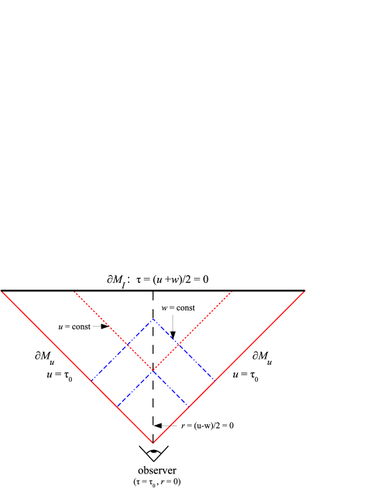
Figure 1: (colour online) An illustration of the manifold $\mathcal{M}$ and its boundary $\partial\mathcal{M}=\partial\mathcal{M}_{u}\cup\partial\mathcal{M}_{I}$ for the general cosmology set-up considered in §III. Here, $\mathcal{M}$ is the causal past of the observer, $\partial\mathcal{M}_{u}$ is the null boundary given by the observer’s past light cone and $\partial\mathcal{M}_{I}$ is a space-like boundary which represents the initial hypersurface. The model remains well-defined in the limit where $\partial\mathcal{M}_{I}$ is the initial singularity. We pick orthogonal null coordinates $u$ and $w$ such that $\partial\mathcal{M}_{u}$ corresponds to $u=\tau_{0}$, and on $\partial\mathcal{M}_{u}$, $-\tau_{0}<w<\tau_{0}$ for some fixed $\tau_{0}$, and the time coordinate given by $\tau=(u+w)/2$ vanishes on $\partial\mathcal{M}_{I}$. We also define a radial coordinate $r=(u-w)/2$ and choose $w=\tau_{0}$ at the observer’s position, so that there $\tau=\tau_{0}$ and $r=0$. In the figure, constant $u$ surfaces are shown as dotted red line (except $\partial\mathcal{M}_{u}$ which is a solid red line), and correspond to past-light cones of points on the line $r=0$ (the dashed black line) which connects the observer with $\partial\mathcal{M}_{I}$. The $w={\rm const}$ surfaces are future-directed light cones of points on $r=0$ and are shown above as dot-dashed blue lines. Surfaces of constant $u$ and $w$ are closed 2-surfaces $S_{(u,w)}$ with intrinsic coordinates $\theta^{i}$; $i=1,2$.

We define a time-like coordinate $\tau=(u+w)/2$. The initial hypersurface therefore corresponds to $\tau=0$ and the observer’s position is $\tau=\tau_{0}$. The normal to $\partial\mathcal{M}_{I}$ is taken to be given, and this therefore partially restricts the freedom in the definition of $u$ and $w$. We also define a space-like radial coordinate $r=(u-w)/2$; we then have $r=0$ at $p_{0}$. FIG. 1 shows an illustration of $\mathcal{M}$ and its boundary.

The intrinsic three-metric on the initial hypersurface has line-element

$$\,\mathrm{d}s_{\tau=0}^{2} = e^{2\sigma_{(I)}}\left(\,\mathrm{d}r^{2}+\bar{h}_{ij}^{(I)}D_{(I)}\theta^{i}D_{(I)}\theta^{j}\right),$$

$$D_{(I)}\theta^{i} = \mathrm{d}\theta^{i}+K_{(I)}^{i}\,\mathrm{d}r,$$

where $\sigma_{(I)}=\left.\sigma\right|_{\tau=0}$, $\bar{h}_{ij}^{(I)}=\left.e^{-2\sigma}h_{ij}\right|_{\tau=0}$ and $K_{(I)}^{i}=\left.r^{i}-s^{i}\right|_{\tau=0}$. The requirement that the initial state be fixed independently of $\lambda$ on $\partial\mathcal{M}_{I}$ implies that $\sigma_{I}$, $\bar{h}_{ij}^{(I)}$ and $K_{I}^{i}$ are fixed up to $\lambda$ independent diffeomorphisms on $\partial\mathcal{M}_{I}$.

The surfaces $S_{(u,w)}$ of constant $u$ and $w$ (or equivalently constant $\tau$ and $r$) represent the intersection of a past and a future-directed light cone. As such, the $S_{(u,w)}$ are closed two-surfaces. We define $\bar{\mathcal{R}}$ to be the scalar curvature of the conformal 2-metric $\bar{h}_{ij}$. Since $\bar{h}_{ij}$ describes a two-dimensional space, it is completely characterized by $\bar{\mathcal{R}}$. Additionally, by the Gauss-Bonnet theorem, we know that

$$\langle\bar{\mathcal{R}}\rangle_{(u,w)}A_{2}(u,w) \equiv \int_{u,w=\mathrm{const}}\bar{\mathcal{R}}\sqrt{\bar{h}}\,\mathrm{d}^{2}\theta$$

$$= 2\int_{u,w=\mathrm{const}}\sqrt{\bar{h}}\,\mathrm{d}^{2}\theta\equiv 2A_{2}(u,w).$$

where $A_{2}(u,w)$ is the surface area of the conformal 2-space described by $\bar{h}_{ij}$, and $\langle\bar{\mathcal{R}}\rangle_{(u,w)}$ is the average curvature. The conformal 2-surfaces are homotopic to a 2-sphere. If the intrinsic metric on the 2-spheres were that of a two-sphere with conformal radius $\rho$, then we would have $A_{2}(u,w)=4\pi\rho^{2}$ and $\langle\bar{\mathcal{R}}\rangle_{(u,w)}=2/\rho^{2}$. This singles out a preferred class of definitions for $u$ and $w$ on the initial hypersurface on which $\tau=(u+w)/2=0$. We can always pick $r=(u-w)/2$ so that on $\partial\mathcal{M}_{I}$ (where $u=-w$), $A_{2}(-w,w)=4\pi r^{2}$ or equivalently $\langle\bar{\mathcal{R}}\rangle_{(-w,w)}=2/r^{2}$.

We note that for a 2-metric, with constant $r$, the diffeomorphism invariant structure of $\bar{h}_{ij}^{(I)}$ is completely determined by its scalar curvature $\bar{\mathcal{R}}_{(I)}$. Since $(u,w)=\mathrm{const}$ represents the intersection of two light cones, the surfaces of constant $u$ and $w$ are closed, and so $\bar{\mathcal{R}}_{(I)}>0$. We note that we can always choose $u$ and $w$ so that on $\partial\mathcal{M}_{I}$, $\bar{\mathcal{R}}_{(I)}=2/r^{2}$ with $r=u=-w$ on $\partial\mathcal{M}_{I}$.

Choice of Surface Terms:

Another freedom in our scheme is the choice of surface terms in $I_{\mathrm{tot}}$. Focussing on the variation of the metric, and keeping all other fields including the CC fixed, these surface terms determine the quantities that must be held on $\partial\mathcal{M,}$ so that $\delta I_{\mathrm{tot}}/\delta g_{\mu\nu}=0$ when the classical field equations hold. The metric on and around a space-like and time-like boundary is described by the induced metric $\gamma_{\mu\nu}$ and the extrinsic curvature, $K^{\mu\nu}$. On a null boundary the situation is slightly more complicated and we discuss it further below; nonetheless, there are quantities analogous to $\gamma_{\mu\nu}$ and $K^{\mu\nu}$. The $\gamma_{\mu\nu}$ and $K^{\mu\nu}$ are respectively analogous to position variables and their associated momenta. In most cases it is natural to choose the surface terms so that (for fixed CC), the ‘position variable’ $\gamma_{\mu\nu}$ must be held fixed. The required surface term was first identified by York York:1972sj , and then rediscovered and refined by Gibbons and Hawking Gibbons:1976ue . We refer to ii as the Gibbons-Hawking-York (GHY) boundary term. However, if $K^{\mu\nu}$, (or some components of it), diverge faster than $\gamma_{\mu\nu}$ as one approaches the boundary, different choices of boundary term may be required.

Metric quantities are suitably well-behaved on the null boundary $\partial\mathcal{M}_{u}$ and so for this boundary it is natural to pick the null boundary analogue of the GHY term.

In the cosmological setting, $\partial\mathcal{M}_{I}$ is the initial singularity and the intrinsic metric, $\gamma_{\mu\nu}^{(0)}$, on $\partial\mathcal{M}_{I}$ has vanishing determinant. More formally, taking $\gamma_{\mu\nu}^{(\tau)}$, to be the induced metric on surfaces of constant $\tau$, $\lim_{\tau\rightarrow 0^{+}}\mathrm{det}\gamma^{(\tau)}=0$. We define $K_{(\tau)}^{\mu\nu}$ to be the extrinsic curvature on constant $\tau$ surfaces; $K_{(\tau)}=K^{\mu}{}_{(\tau)\mu}$. Generally, $K$ diverges as $\tau\rightarrow 0^{+}$. The quantities $\mathrm{det}\gamma$ and $K$ are canonically conjugate. It is most natural to choose boundary terms so that the most divergence of two canonically conjugate variables is held fixed (c.f. the argument for fixing the charge rather than the chemical potential in Ref. Sen:2008yk ). This implies that, on $\partial\mathcal{M}_{I}$, we choose the surface term so that $K$ rather than $\mathrm{det}\gamma$ is fixed. In Appendix B, we note that this term is the ‘cosmological’ boundary term found by York in Ref. York:1972sj . Thus, we fix the surface terms in $I_{\mathrm{tot}}$ to be York’s cosmological boundary term on $\partial\mathcal{M}_{I}$, and the GHY boundary term on $\partial\mathcal{M}_{u}$. It should be stressed, though, this choice of York rather tha GHY boundary term on $\partial\mathcal{M}_{I}$ has no affect on the equation for $\lambda$ and is only made for the technical reason stated above. This is because the initial state on $\partial\mathcal{M}_{\rm I}$ is fixed independently of $\lambda$ in our proposal and so for any $\partial\mathcal{M}_{I}$ boundary term, $I_{\partial\mathcal{M}_{I}}$, $\delta I_{\rm dM_{I}}/\delta\lambda=0$. It follows that boundary terms on $\partial\mathcal{M}_{I}$ do not contribute to the $\lambda$-equation: $\delta I_{\rm tot}/\delta\lambda=0$.

III.1 General Cosmology

We begin by writing down the form of $I_{\mathrm{tot}}$ for the general cosmological setting and considering its variation. In addition to $I_{\mathrm{tot}}$, our scheme requires that we specify a set of quantities $\left\{Q^{A}\right\}$ that are kept fixed (for all values of the bare cosmological constant) and which can be independently specified. By considering the variation of the action, we present a natural choice of these fixed quantities.

Since we have taken the gravity sector to be described (to a suitable approximation) by unmodified general relativity, the gravitational action, $I_{\mathrm{grav}}$, is given by

$$I_{\mathrm{grav}}[g_{\mu\nu};\mathcal{M}]=I_{\mathrm{EH}}[g_{\mu\nu};\mathcal{M}]+I_{\mathrm{surf}}[g_{\mu\nu};\partial\mathcal{M}],$$

where $I_{\mathrm{surf}}$ are the surface terms defined on $\partial\mathcal{M}$ and $I_{\mathrm{EH}}$ is the Einstein-Hilbert action defined on $\mathcal{M}$:

$$I_{\mathrm{EH}}[g_{\mu\nu};\mathcal{M}]=\frac{1}{2\kappa}\int_{\mathcal{M}}\,\mathrm{d}^{4}x\,\sqrt{-g}R(g).$$

We have taken the boundary to be $\partial\mathcal{M}=\partial\mathcal{M}_{(u)}\cup\partial\mathcal{M}_{I}$, where $\partial\mathcal{M}_{(u)}$ is described by the vanishing of the null coordinate $u$, and so it represents a null boundary. Our $\partial\mathcal{M}_{I}$ is the initial space-like hypersurface given by $\tau=0$. As one approaches $\tau=0$, the determinant of the induced metric on $\tau=\mathrm{const}$ hypersurfaces vanishes, whilst the trace of the extrinsic curvature diverges. On $\partial\mathcal{M}_{(u)}$ it is natural to take the surface term to be the null boundary analogue of the Gibbons-Hawking-York (GHY) term, $I_{\mathrm{GHY}}^{(u)}$ say, whereas on $\partial\mathcal{M}_{I}$ the divergence of $K$ makes $\tau\rightarrow 0$ limit of York’s cosmological (YC) surface more natural; we write this as $I_{\mathrm{YC}}^{(I)}$.

In appendix B we present a detailed rederivation and discussion of boundary terms in general relativity for both non-null and null boundaries. Here, we briefly review those results where they apply to the form of the $I_{\mathrm{GHY}}^{(u)}$ and $I_{\mathrm{YC}}^{(I)}$ terms.

III.1.1 GHY term on $\partial\mathcal{M}_{u}$ ($u=\tau_{0}$):

We consider a null boundary $\partial\mathcal{M}_{(u)}$ described by some $u(x^{\mu})=\tau_{0}$ where, with $u_{\mu}=\nabla_{\mu}u$, we have $u^{\mu}u_{\mu}=0$. We define $n^{\mu}=-e^{\sigma}u^{\mu}$ for some $\sigma$. In order to describe points on $\partial\mathcal{M}_{(u)},$ we have a $w(x^{\mu})$ such that $w_{\mu}=\nabla_{\mu}w$ is null and $w_{\mu}u^{\mu}=-2e^{-2\sigma}>0$. We also define $\tau=(u+w)/2$ and so, on $\partial\mathcal{M}_{u}$, $\tau=(\tau_{0}+w)/2$. Eq. (5) gives the decomposition of the metric $g_{\mu\nu}$ in terms of $u$, $w$ and the intrinsic coordinates $\theta^{i}$ on the closed 2-surfaces, $S_{(u,w)}$, of constant $u$ and $w$. The $h_{ij}$ is the induced 2-metric on the $S_{(u,w)}$ and $h_{\mu\nu}=g_{\mu\nu}-e^{2\sigma}w_{(\mu}u_{\nu)}$. We define $n^{\mu}=-e^{\sigma}u^{\mu}$, and $\bar{n}^{\mu}=e^{\sigma}w^{\mu}$ so that $\bar{n}^{\mu}n_{\mu}=2$.

The extrinsic curvature of $S_{(u,w)}$ along $n^{\mu}$ is $\mathcal{K}^{\mu\nu}$ and is defined by

$$\mathcal{K}^{\mu\nu} = -\frac{1}{2}h^{\mu\rho}h^{\nu\sigma}\mathcal{L}_{n}h_{\rho\sigma}$$

$$= e^{\sigma}h^{\mu\rho}h^{\nu\sigma}\nabla_{\rho}u_{\sigma}.$$

Writing $e_{\mu}^{i}=\partial_{\mu}\theta^{i}$, we define $\mathcal{K}^{ij}=e_{\mu}^{i}e_{\nu}^{j}\mathcal{K}^{\mu\nu}$ and the trace of the extrinsic curvature is $\mathcal{K}=\mathcal{K}^{\mu\nu}h_{\mu\nu}=\mathcal{K}^{ij}h_{ij}$. We also define the inaffinity, $\nu$, and twist, $\omega^{\mu}$, by

$$\nu=-\mathcal{L}_{n}\sigma=e^{\sigma}u^{\mu}\nabla_{\mu}\sigma,\qquad\omega^{\mu}=\frac{1}{2}h^{\mu\nu}\bar{n}_{\rho}\nabla_{\nu}n^{\rho}.$$

We also define $\omega^{i}=\omega^{\mu}e_{\mu}^{i}$.

The usual GHY term (defined on non-null boundaries) has the property that it renders the action first order in derivatives of the metric. The variation of the total action with respect to the metric is then free of surface terms whenever the induced boundary 3-metric is held fixed. On a null boundary there is no (non-singular) boundary 3-metric. In its place are $h_{\mu\nu}$ and $e^{\sigma}$. This is clear when one notes that the invariant area element on $\partial\mathcal{M}_{(u)}$ is $e^{\sigma}\sqrt{h}\,\mathrm{d}\tau\,\mathrm{d}^{2}\theta$, as opposed to $\sqrt{|\gamma|}\,\mathrm{d}^{3}x$ on a non-null boundary. Thus, the analogue of the GHY term for a null boundary is defined by the property that when $e^{\sigma}$ and $h_{\mu\nu}$ are fixed, variation of the total action with respect to the metric is free of surface terms on $\partial\mathcal{M}_{u}$.

Given this, we find in Appendix B that the GHY term for $\partial\mathcal{M}_{(u)}$ is:

$$I_{\mathrm{GHY}}^{(u)}=\frac{1}{\kappa}\int_{\partial\mathcal{M}_{u}}e^{\sigma}\sqrt{h}\,\mathrm{d}\tau\,\mathrm{d}^{2}\theta\,\left[\mathcal{K}+\nu\right].$$

One finds the same boundary term if one starts with the EH action in terms of a vierbein and adds a boundary term so that action is first order in derivatives of the vierbein (see Appendix B for a proof of this).

On a space-like or time-like boundary, $\Sigma$ say, it is well known that the GHY boundary term invariant under diffeomorphisms restricted to $\Sigma$ (i.e. those under which the 4-vector normal to $\Sigma$ is invariant). However, on a null boundary this is not the case. $I_{\mathrm{GHY}}^{(u)}$ is invariant under diffeomorphisms on the two surfaces of constant $u$ and $w$ (i.e. $S_{(u,w)}$), but it is not invariant under reparametrizations of the ‘radial’ coordinate (in this case $w$ or equivalently $\tau$, along the null hypersurface). Specifically, it is always possible to find such diffeomorphisms that preserve the normal to $\partial\mathcal{M}_{(u)}$ but under which

$$\left.\nu\right|_{\partial\mathcal{M}_{u}}\rightarrow\left.\nu\right|_{\partial\mathcal{M}_{u}}+e^{\sigma}\mathcal{L}_{u}f_{-}(w,\theta^{i}).$$

for any $f_{-}(w,\theta^{i})$. This means that the $I_{\mathrm{GHY}}^{(u)}$ term as defined above is ambiguous. The ambiguity in the GHY term for null boundaries is because the 3-metric normal to the boundary is degenerate. This means that there is no preferred normalization of the normal to the boundary and consequently no preferred ‘radial’ coordinate along the boundary. To unambiguously define the $I_{\mathrm{GHY}}^{(u)}$ one must fix this remaining gauge freedom by either picking a form for $\nu$ on $\partial\mathcal{M}_{(u)}$ or, equivalently, by specifying a preferred choice of $w$/$\tau$ on $\partial\mathcal{M}_{u}$. Simplifying choices that are common in the literature, and can always be achieved, are

$$\left.\nu\right|_{\partial\mathcal{M}_{u}}=0\,\qquad\mathrm{or}\qquad\left.\nu\right|_{\partial\mathcal{M}_{u}}=-\frac{c_{0}}{2}\mathcal{K},$$

for some constant $c_{0}$. Each choice identifies a preferred $w$ for which the total action is first order in derivatives of metric quantities. In this application of our proposal to solve the CC problems, we demand that the initial state is fixed independent of $\lambda$. However, both these choices for $\nu$ on $\partial\mathcal{M}_{u}$ given above would single out a preferred $w$, and hence a definition of $\sigma$ which would depend on $\lambda$ on $\partial\mathcal{M}_{I}$. In the scenario we consider here, it is more natural to remove the ambiguity in $\nu$ on $\partial\mathcal{M}_{u}$ by fixing the definition of $\sigma$ initially (i.e. on $\partial\mathcal{M}_{I}$). This is achieved by picking a preferred radial coordinate $r$ on $\partial\mathcal{M}_{I}$. More exactly, we should specify the $r$ on $\partial\mathcal{M}_{I}$ up to residual coordinate transformations that leave $I_{\mathrm{GHY}}^{(u)}$ invariant. We noted above that since the $S_{(u,w)}$, which are the surfaces of constant $r$ on $\partial\mathcal{M}_{I}$, are closed 2-surfaces, our $r$ represents a radial coordinate on $\partial\mathcal{M}_{I}$. A simple and natural definition of $r$ (up to residual coordinate transformations) is then to pick it so that the average scalar curvature of the conformal 2-surface at $\tau=0$ and $r=\mathrm{const}$ (and described by the metric $\bar{h}_{ij}=e^{-2\sigma}h_{ij})$ is $2/r^{2}$ with $r=u=-w$ on $\partial\mathcal{M}_{I}$. By the Gauss-Bonnet theorem, this is equivalent choosing $r$ so that the surface area of the conformal 2-surface is $4\pi r^{2}$. This choice does not uniquely determine $r$ but it is sufficient to fix $\nu$ on $\partial\mathcal{M}_{u}$.

The choice of a preferred $r$ on $\partial\mathcal{M}_{I}$ is equivalent to the specification of an unambiguous boundary term on $\partial\mathcal{M}_{u}$. Making such a specification requires that one replace $\nu$ in $I_{\mathrm{GHY}}^{(u)}$ by some quantity that is invariant under diffeomorphisms that vanish normal to $\partial\mathcal{M}_{u}$ and $\partial\mathcal{M}_{I}$. Any such choice will then pick out a preferred set of definitions of $w$ on $\partial\mathcal{M}_{u}$ for which $\nu=-\mathcal{L}_{n}\sigma$ and hence the total action is first order. This in turns picks out a preferred set of $2r=(u-w)$ on $\partial\mathcal{M}_{I}$ where $w=-u$. For the application of our proposal to cosmology in this section we fix the definition of $\nu$ so that on $\partial\mathcal{M}_{I}$, $\left\langle\bar{\mathcal{R}}\right\rangle_{\tau=0}=2/r^{2}$. This is arguably the simplest choice we can make that is consistent with the requirement that the initial state be $\lambda$ independent when described in the coordinate chart for which the action is (up to a boundary term on $\partial\mathcal{M}_{I}$) first order in metric derivatives.

III.1.2 YC term on $\partial\mathcal{M}_{I}$ ($\tau=0$):

The initial time-like hypersurface, $\partial\mathcal{M}_{I}$, is singular, however we may still define the surface term by taking a limit as $\tau\rightarrow 0$ from above (i.e. $\tau\rightarrow 0^{+}$). We take $t^{\mu}=e^{\sigma}\nabla^{\mu}\tau$ where $\tau=(u+w)/2$. We then have $t^{\mu}t_{\mu}=-1$; $t^{\mu}$ is the backward pointing normal to surfaces, $\Sigma_{\tau}$, of constant $\tau$. We can decompose the metric into

$$g_{\mu\nu}=-t_{\mu}t_{\nu}+\gamma_{\mu\nu}.$$

With $r=(u-w)/2,$ we have:

$$\gamma_{\mu\nu}\,\mathrm{d}x^{\mu}\,\mathrm{d}x^{\nu}=e^{2\sigma}\,\mathrm{d}r^{2}+h_{ij}\left[\,\mathrm{d}\theta^{i}+K^{i}\,\mathrm{d}r\right]\left[\,\mathrm{d}\theta^{j}+K^{j}\,\mathrm{d}r\right],$$

where $K^{i}=(r^{i}-s^{i})$. The $\theta^{i}$ are the intrinsic coordinates on the surfaces of constant $u$ and $w$. The line element for the 4-metric can then be written as

$$\,\mathrm{d}s^{2}=-e^{\sigma}\,\mathrm{d}\tau^{2}+\gamma_{\alpha\beta}\left[\,\mathrm{d}x^{\alpha}+N^{\alpha}\,\mathrm{d}\tau\right]\left[\,\mathrm{d}x^{\beta}+N^{\beta}\,\mathrm{d}\tau\right],$$

where

$$N_{\alpha}\,\mathrm{d}x^{\alpha}=h_{ij}(r^{j}+s^{j})\,\mathrm{d}\theta^{i}.$$

We call $N^{\alpha}$ the shift-vector. We note that we can always define the $\theta^{i}$ so that in $\mathcal{M}$, $N^{\alpha}=0$ i.e. $r^{i}=-s^{i}$. The extrinsic curvature, $K^{\mu\nu}$, of $\ \Sigma_{\tau}$ is given by

$$K^{\mu\nu}=-\frac{1}{2}\gamma^{\mu\rho}\gamma^{\nu\sigma}\mathcal{L}_{t}\gamma_{\rho\sigma},$$

and the trace is $K=K^{\mu\nu}\gamma_{\mu\nu}$. With these definitions we see in Appendix B that the cosmological boundary term of York for $\partial\mathcal{M}_{I}$ is:

$$I_{\mathrm{YC}}^{(I)}=-\lim_{\tau\rightarrow 0^{+}}\frac{1}{3\kappa}\int_{\partial\mathcal{M}_{I}}\sqrt{\gamma}\,\mathrm{d}^{3}x\,K.$$

III.1.3 Variation of Gravitational Action and Fixed Quantities:

In this cosmological set-up the total gravitational action is:

$$I_{\mathrm{grav}} = \frac{1}{2\kappa}\int_{\mathcal{M}}\,\mathrm{d}^{4}x\,\sqrt{-g}R(g)$$

$$+\frac{1}{\kappa}\int_{\partial\mathcal{M}_{u}}e^{\sigma}\sqrt{h}\,\mathrm{d}\tau\,\mathrm{d}^{2}\theta\,\left[\mathcal{K}+\nu\right]$$

$$-\lim_{\tau\rightarrow 0^{+}}\frac{1}{3\kappa}\int_{\partial\mathcal{M}_{I}}\sqrt{\gamma}\,\mathrm{d}^{3}x\,K.$$

In appendix B we show that the variation of this action with respect to the metric, $g_{\mu\nu}$, gives:

$$\delta I_{\mathrm{grav}} = -\frac{1}{2\kappa}\int_{\mathcal{M}}\,\mathrm{d}^{4}x\,\sqrt{-g}G^{\mu\nu}\delta g_{\mu\nu}$$

$$-\frac{1}{2\kappa}\int_{\partial\mathcal{M}_{I}}\left[\tilde{P}^{\alpha\beta}\delta\tilde{\gamma}_{\alpha\beta}+\frac{4}{3}\sqrt{\gamma}\delta K\right]\,\mathrm{d}r\,\mathrm{d}^{2}\theta,$$

$$+\frac{1}{2\kappa}\int_{\partial\mathcal{M}_{u}}e^{\sigma}\sqrt{h}\left[(\mathcal{K}+\nu)h^{ij}-\mathcal{K}^{ij})\delta h_{ij}\right.$$

$$+\left.2\mathcal{K}\delta\sigma+2\omega_{i}\delta s^{i}\right]\,\mathrm{d}\tau\,\mathrm{d}^{2}\theta,$$

where

$$\tilde{\gamma}_{\alpha\beta} = (\mathrm{det}\,\gamma)^{-1/3}\gamma_{\alpha\beta},$$

$$\tilde{P}^{\alpha\beta} = (\mathrm{det}\,\gamma)^{5/6}\left[K^{\alpha\beta}-\frac{1}{3}K\gamma^{\alpha\beta}\right].$$

Since $\tilde{P}^{\alpha\beta}\tilde{\gamma}_{\alpha\beta}=0$, it follows that:

$$\tilde{P}^{\alpha\beta}\delta\tilde{\gamma}_{\alpha\beta} = -\tilde{\gamma}_{\alpha\beta}\delta\tilde{P}^{\alpha\beta}=-\sqrt{\gamma}\gamma_{\alpha\beta}\delta\sigma^{\alpha\beta},$$

$$\sigma^{\alpha\beta} = K^{\alpha\beta}-\frac{1}{3}K\gamma^{\alpha\beta}.$$

We now specify the fixed quantities, $\left\{Q^{A}\right\}$, for the gravitational sector. We see that the boundary terms in Eq. (III.1.3) vanish when $K$ and either $\tilde{\gamma}_{\alpha\beta}$ or $\sigma^{\alpha\beta}$ are fixed on $\partial\mathcal{M}_{I}$ (up to residual coordinate transformations on $\partial\mathcal{M}^{I}$) and $s^{i}$ , $h_{ij}$ and $\sigma$ are fixed on $\partial\mathcal{M}_{u}$. The $\left\{Q^{A}\right\}$ will be a subset of these quantities, and their defining property is that they are a maximal subset which can be independently specified.

In terms of the familiar 3+1 ADM decomposition on constant time (i.e. $\tau$) hypersurfaces, $\Sigma_{\tau}$, our $e^{\sigma}$ is the lapse function and $N^{\alpha}=(0,r^{i}+s^{j})$ is the shift vector; $\gamma_{\alpha\beta}$ is the induced metric on $\Sigma_{\tau}$. The six components of $\gamma_{\alpha\beta}$ are given by $\sigma$, $K^{i}=r^{i}-s^{i},$ and $h_{ij}$.

In general, the intrinsic coordinate-independent geometry in $\mathcal{M}$ is determined uniquely when the twelve variables $\gamma_{\alpha\beta}$ and $K^{\alpha\beta}$ are specified on $\partial\mathcal{M}_{I}$. The Einstein equations provide four constraint equations on $\partial\mathcal{M}_{I}$ which reduce the number of independent functions in $\gamma_{\alpha\beta}$ and $K^{\alpha\beta}$ to eight. When $N=e^{\sigma}$ and $N^{\alpha}$ in $\mathcal{M}$ are fixed, this reduces the number of independent functions that must be specified on $\partial\mathcal{M}_{I}$ to four. Thus, to completely specify the space-time in $\mathcal{M}$, we must fix four free functions on $\partial\mathcal{M}_{I}$ as well as specifying $N$ and $N^{\alpha}$ in $\mathcal{M}$.

The specification of $\tilde{\gamma}_{\alpha\beta}$ (or $\sigma^{\alpha\beta}$) and $K$ on $\partial\mathcal{M}_{I}$ fixes six functions on the initial hypersurface in a coordinate dependent manner. We found that the definition of $I_{\mathrm{GHY}}^{(u)}$ resulted in the specification of a preferred $r$ on $\partial\mathcal{M}_{I}$. There remains, however, the freedom to define the $\theta^{i}$ on $\partial\mathcal{M}_{I}$ which can be used, for instance, to set $K^{i}=0$ initially. This freedom means that $\tilde{\gamma}_{\alpha\beta}$ (or $\sigma^{\alpha\beta}$) and $K$ on $\partial\mathcal{M}_{I}$ fix four free functions on $\partial\mathcal{M}_{I}$ in a coordinate independent manner. The lapse function, $N$, in $\mathcal{M}$ to be given by $N=e^{\sigma}$. If $N^{\alpha}$ can be fixed in $\mathcal{M}$, then $\tilde{\gamma}_{\alpha\beta}$ (or $\sigma^{\alpha\beta}$) and $K$ on $\partial\mathcal{M}_{I}$ are sufficient to completely determine, via the field equations, all metric quantities in $\mathcal{M}$, and on $\partial\mathcal{M}_{u}$. Fixing $N^{\alpha}$ in terms other metric quantities is equivalent to fixing $r^{i}+s^{i}$ which in turn is equivalent to specifying our coordinates $\theta^{i}$ on $S_{(u,w)}$ which are defined on surfaces of constant $\tau$ relative to their values on $\partial\mathcal{M}_{I}$. A simple choice with a geometrical basis is demand that the $\theta^{i}$ are Lie-propagated along $\tau^{\mu}=\nabla^{\mu}\tau$ from the values that are arbitrarily assigned to them on the initial hypersurface $\partial\mathcal{M}_{I}$ i.e. $\mathcal{L}_{\tau}\theta^{i}=0$. This implies that:

$$\mathcal{L}_{\tau}\theta^{i}=\frac{1}{2}\left(u^{\mu}\partial_{\mu}\theta^{i}+w^{\mu}\partial_{\mu}\theta^{i}\right)=e^{-2\sigma}(r_{i}+s_{i})=0,$$

and so $r_{i}=-s_{i}$ in $\mathcal{M}$. We then have $N^{\alpha}=0$. We make this choice in our subsequent analysis.

Our choice of fixed quantities, $\left\{Q^{A}\right\}$, is therefore as follows:

• We assume that the initial state on $\partial\mathcal{M}_{I}$ is fixed. Thus, the fixed $\left\{Q^{A}\right\}$ include $K$ and either $\tilde{\gamma}_{\mu\nu}$ or $\sigma^{\alpha\beta}$ on $\partial\mathcal{M}_{I}$.

• These quantities are fixed with respect to a $\lambda$-independent coordinate chart $\mathcal{C}=\left\langle u,w,\theta^{1},\theta^{2}\right\rangle$ defined such that $u=\tau_{0}=\mathrm{fixed}$ on $\partial\mathcal{M}_{I}$, $w=\tau_{0}=\mathrm{fixed}$ at $p_{0}$ and $u=-w$ on $\partial\mathcal{M}_{I}$. $\partial\mathcal{M}_{I}$ has fixed unit normal $t_{I}^{\mu}=\left.e^{-\sigma}\tau^{\mu}\right|_{\partial\mathcal{M}_{I}}$; $\tau^{\mu}=\nabla^{\mu}(u+w)/2$.

• We found that an invariant definition of the boundary term on $\partial\mathcal{M}_{u}$ requires us to pick out a preferred set of $r=(u-w)/2$ on $\partial\mathcal{M}_{I}$. Our choice of $r$ is to define it so that $e^{-2\sigma}r^{-2}h_{ij}$ has an average scalar curvature of $2$ on $\partial\mathcal{M}_{I}$.

• The values $\theta^{i}$ in $\mathcal{M}$ are defined by Lie-propagating their values on $\partial\mathcal{M}_{I}$ along $\tau^{\mu}$: $\mathcal{L}_{\tau}\theta^{i}=0$ and so $r^{i}=-s^{i}$ everywhere.

Similarly, for the matter variables, we fix the initial state on $\partial\mathcal{M}_{I}$ and any residual gauge freedom on $\partial\mathcal{M}_{u}$, so that the gauge is fixed independently of $\lambda$.

Given this choice $\left\{Q^{A}\right\}$, the 2-metric, $h_{ij}$, on $\partial\mathcal{M}_{u}$ is determined by the classical field equations. Since the field equations depend on $\Lambda$, this, in turn, fixes the form of $\mathcal{H}_{ij}\equiv\,\mathrm{d}h_{ij}/\,\mathrm{d}\lambda$.

III.1.4 The $\Lambda$ field equation:

The field equation for $\Lambda$ in our proposed paradigm is Eq. (3). Here, the total action is

$$I_{\mathrm{tot}}=I_{\mathrm{grav}}[g_{\mu\nu}]+I_{\mathrm{CC}}[\Lambda,g_{\mu\nu};\mathcal{M}]+I_{\mathrm{matter}}[\Psi^{a},g_{\mu\nu};\mathcal{M}].$$

where $I_{\mathrm{grav}}=I_{\mathrm{EH}}+I_{\mathrm{GHY}}^{(u)}+I_{\mathrm{YC}}^{(I)}$. We assume that $I_{\mathrm{matter}}$ is of the form

$$I_{\mathrm{matter}}=\int_{\mathcal{M}}\sqrt{-g}\mathcal{L}_{\mathrm{matter}}+\int_{\partial\mathcal{M}_{I}}\sqrt{\gamma}\,\mathrm{d}^{3}x\mathcal{L}_{\mathrm{mI}},$$

for some $\mathcal{L}_{\mathrm{mI}}$, where $\mathcal{L}_{\mathrm{matter}}$ and $\mathcal{L}_{\mathrm{mI}}$ are at most first order in derivatives of $\Psi^{a}$. The choice of fixed quantities $\left\{Q^{A}\right\}$ define the initial state and ensure all integrals over $\partial\mathcal{M}_{I}$ in $\delta I_{\mathrm{tot}}$ vanish. The classical field equations for gravity and matter are

$$E^{\mu\nu} = -G^{\mu\nu}+\kappa T^{\mu\nu}-\Lambda g^{\mu\nu},$$

$$\Psi^{a} = -\nabla_{\mu}\Pi_{a}^{\mu}+\frac{\delta\mathcal{L}_{\mathrm{matter}}}{\delta\Psi^{a}}=0,$$

where

$$T^{\mu\nu}=\frac{2}{\sqrt{-g}}\frac{\delta(\sqrt{-g}\mathcal{L}_{\mathrm{matter}})}{\delta g_{\mu\nu}},\qquad\Pi_{a}^{\mu}=\frac{\delta\mathcal{L}_{\mathrm{matter}}}{\delta(\nabla_{\mu}\Psi^{a})}.$$

Combined with these classical field equations, the fixed $\left\{Q^{A}\right\}$ determine $h_{ij}$ and $\Psi^{a}$ on $\partial\mathcal{M}_{u}$ as functions of $\Lambda$. Thus, they give

$$\mathcal{H}_{ij}=\left.\frac{\,\mathrm{d}h_{ij}}{\,\mathrm{d}\Lambda}\right|_{\partial\mathcal{M}_{u};\mathrm{fixed}\,\,\left\{Q^{A}\right\}},\qquad\mathcal{P}^{a}=\left.\frac{\,\mathrm{d}\Psi^{a}}{\,\mathrm{d}\Lambda}\right|_{\partial\mathcal{M}_{u};\mathrm{fixed}\,\,\left\{Q^{A}\right\}}.$$

When $g_{\mu\nu}$ and $\Psi^{a}$ obey $E^{\mu\nu}=\Psi^{a}=0$, we have $I_{\mathrm{tot}}=I_{\mathrm{class}}[\Lambda;\mathcal{M}]$ and so Eq. (3) reads

$$\frac{\,\mathrm{d}I_{\mathrm{class}}}{\,\mathrm{d}\Lambda} = \frac{1}{2\kappa}\int_{\partial\mathcal{M}_{u}}N\sqrt{h}\,\mathrm{d}\tau\,\mathrm{d}^{2}\theta\left[\mathcal{N}^{ij}\mathcal{H}_{ij}+\Sigma_{a}\mathcal{P}^{a}\right]$$

$$-\frac{1}{\kappa}\int_{\mathcal{M}}\sqrt{-g}\,\mathrm{d}^{4}x=0.$$

where $\mathcal{N}^{ij}=(\mathcal{K}+\nu)h^{ij}-\mathcal{K}^{ij}$ and $\Sigma_{a}=-n_{\mu}\Pi_{a}^{\mu}$.

III.1.5 Rewriting the Classical Action

When the classical field equations for the metric and matter variables hold, we can rewrite $I_{\mathrm{class}}$ in a form that is particularly instructive in the cosmological setting for both expressing and solving the $\lambda$ equation.

Independent of the field equations, we can rewrite $I_{\mathrm{GHY}}^{(u)}$ as

$$\kappa I_{\mathrm{GHY}}^{(u)} = \int_{\partial\mathcal{M}_{u}}e^{\sigma}\sqrt{h}\left[\mathcal{K}+\nu\right]\,\mathrm{d}\tau\,\mathrm{d}^{2}\theta$$

$$= \int_{\partial\mathcal{M}_{u}}\left[\nabla_{\mu}u^{\mu}+u^{\mu}\nabla_{\mu}\sigma\right]\sqrt{-g}\,\mathrm{d}\tau\,\mathrm{d}^{2}\theta$$

$$= -\int_{\mathcal{M}}\sqrt{-g}\nabla_{\mu}\left[t^{\mu}\mathcal{L}_{n}\sigma\right]\,\mathrm{d}^{4}x$$

$$-\lim_{\tau\rightarrow 0^{+}}\int_{\partial\mathcal{M}_{I}}e^{\sigma}\sqrt{h}\mathcal{L}_{n}\sigma\,\mathrm{d}r\,\mathrm{d}^{2}\theta,$$

where we have used $u_{\mu}u^{\mu}=0$, and $\sqrt{-g}=0$ on $\tau=0$ and at $p_{0}$. We have also used $n^{\mu}=-e^{\sigma}u^{\mu}$, $t^{\mu}=e^{\sigma}\nabla^{\mu}\tau$ and $n^{\mu}t_{\mu}=1$. Now,

$$\mathcal{L}_{n}\sigma=n^{\mu}\nabla_{\mu}\sigma=t^{\nu}n^{\mu}\nabla_{\mu}n_{\nu}=-n^{\mu}n^{\nu}\nabla_{\mu}t_{\nu}=-K^{r}{}_{r}-a_{r},$$

where $\nabla_{\mu}t_{\nu}=K_{\mu\nu}-t_{\mu}a_{\nu}$, and $a_{\mu}=t^{\nu}\nabla_{\nu}t^{\mu}$ is the acceleration and $K_{\mu\nu}$ the extrinsic curvature of constant $\tau$ hypersurfaces. We have also defined $l^{\mu}=e^{\sigma}\nabla^{\mu}r=e^{\sigma}\nabla^{\mu}\left[u-w\right]/2$, so that $n^{\mu}=-(t^{\mu}+r^{\mu})$ and $K^{r}{}_{r}=l^{\mu}l^{\nu}K_{\mu\nu}$, $a_{r}=l^{\mu}a_{\mu}$.

Since

$$\lim_{\tau\rightarrow 0^{+}}\left[\int_{\partial\mathcal{M}_{I}}e^{\sigma}\sqrt{h}a_{r}\,\mathrm{d}r\,\mathrm{d}^{2}\theta=\int_{\partial\mathcal{M}_{I}}t_{\mu}n^{\mu}e^{\sigma}\sqrt{h}a_{r}\,\mathrm{d}r\,\mathrm{d}^{2}\theta\right],$$

$$=\int_{\mathcal{M}}\sqrt{-g}\,\mathrm{d}^{4}x\,\nabla_{\mu}\left[n^{\mu}a_{r}\right],$$

we can write:

$$I_{\mathrm{GHY}}^{(u)} = \frac{1}{\kappa}\int_{\mathcal{M}}\sqrt{-g}\nabla_{\mu}\left[t^{\mu}K^{r}{}_{r}-l^{\mu}a_{r}\right]\,\mathrm{d}^{4}x$$

$$+\lim_{\tau\rightarrow 0^{+}}\frac{1}{\kappa}\int_{\partial\mathcal{M}_{I}}e^{\sigma}\sqrt{h}K^{r}{}_{r}\,\mathrm{d}r\,\mathrm{d}^{2}\theta.$$

The Ricci tensor of $\mathcal{M}$ is $R_{\mu\nu}$, and we define $R_{\mu\nu}^{(3)}$ to be the Ricci tensor of a 3-surface of constant $\tau$. We define $R^{r}{}_{r}=R_{\mu\nu}l^{\mu}l^{\nu}$, $R^{(3)r}{}_{r}=R_{\mu\nu}^{(3)}l^{\mu}l^{\nu}$. We then have:

$$\nabla_{\mu}\left[t^{\mu}\mathcal{L}_{n}\sigma-l^{\mu}a_{r}\right] = -R_{r}^{r}+R_{r}^{(3)r}+\mathcal{L}_{l}a_{r}$$

$$+A^{2}-\Sigma^{2}-a_{r}\mathcal{K}_{l},$$

$$\Sigma^{2} = 2\Sigma_{\mu}\Sigma^{\mu},\qquad\Sigma_{\mu}=h_{\mu\nu}l_{\rho}K^{\nu\rho},$$

$$A^{2} = A_{\mu}A^{\mu},\qquad A_{\mu}=h_{\mu\nu}a^{\mu},$$

$$\mathcal{K}_{l} = h^{\mu\nu}\nabla_{\mu}l_{\nu}=\frac{1}{2}h^{\mu\nu}\mathcal{L}_{l}h_{\mu\nu}.$$

We now define:

$$\Gamma\equiv R_{r}^{(3)r}+\mathcal{L}_{l}a_{r}+A^{2}-\Sigma^{2}-a_{r}\mathcal{K}_{l}.$$ (8)

We can then write:

$$I_{\mathrm{tot}} = I_{\mathrm{EH}}+I_{\mathrm{GHY}}^{(u)}+I_{\mathrm{YC}}^{(I)}+I_{CC}+I_{\mathrm{matter}},$$

$$= \frac{1}{\kappa}\int_{\mathcal{M}}\sqrt{-g}\left[\frac{1}{2}R-R^{r}{}_{r}-\Lambda+\Gamma+\kappa\mathcal{L}_{\mathrm{matter}}\right]\,\mathrm{d}^{4}x$$

$$+\lim_{\tau\rightarrow 0^{+}}\frac{1}{\kappa}\int_{\partial\mathcal{M}_{I}}\sqrt{\gamma}\left[K_{r}^{r}-\frac{1}{3}K+\mathcal{L}_{\mathrm{mI}}\right]\,\mathrm{d}^{3}x.$$

$I_{\mathrm{class}}$ is defined to be $I_{\mathrm{tot}}$ evaluated with $g_{\mu\nu}$ and the matter fields obeying their classical field equations. For $g_{\mu\nu}$ this means that we have the Einstein equation $G_{\mu\nu}=R_{\mu\nu}-g_{\mu\nu}R/2=\kappa T^{\mu\nu}-\Lambda g_{\mu\nu}$ where $T^{\mu\nu}$ is the energy-momentum tensor that follows from varying $\mathcal{L}_{\mathrm{matter}}$. Substituting the Einstein equation into $I_{\mathrm{tot}}$ and defining $P^{r}{}_{r}=T_{\mu\nu}l^{\mu}l^{\nu}$ we arrive at:

$$I_{\mathrm{class}} = \int_{\mathcal{M}}\sqrt{-g}\left[\kappa^{-1}\Gamma+(\mathcal{L}_{\mathrm{matter}}-P^{r}{}_{r})\right]\,\mathrm{d}^{4}x$$

$$+\lim_{\tau\rightarrow 0^{+}}\frac{1}{\kappa}\int_{\partial\mathcal{M}_{I}}\sqrt{\gamma}\left[K_{r}^{r}-\frac{1}{3}K+\mathcal{L}_{\mathrm{mI}}\right]\,\mathrm{d}^{3}x.$$

Since the initial state on $\partial\mathcal{M}_{I}$ is taken to be fixed, the equation for the effective cosmological constant $\Lambda$ can be simply written as:

$$\frac{\,\mathrm{d}I_{\mathrm{class}}}{\,\mathrm{d}\lambda} = \int_{\mathcal{M}}\frac{\delta}{\delta\Lambda}\left\{\sqrt{-g}\left[\kappa^{-1}\Gamma+(\mathcal{L}_{\mathrm{matter}}-P^{r}{}_{r})\right]\right\}\,\mathrm{d}^{4}x$$

$$= 0.$$

In the above equation $\mathcal{L}_{\mathrm{matter}}$ is the effective action for matter renormalized so that it vanishes in vacuo. In a cosmological setting, this form of the $\Lambda$ equation is often the most straightforward to evaluate since it involves only scalar quantities.

III.2 $\Lambda$ in a Realistic Cosmology

In the previous subsection, we considered the application of our scheme for determining $\Lambda$ in a general cosmological setting where $\mathcal{M}$ is taken to be the past light cone of the observer at some fixed external time $\tau=\tau_{0}$.

We assume that, in appropriate coordinates $(T,X^{i})$, and except in certain strong gravity regimes (eg. near neutron stars or black hole horizons), the space-time is well-described, to linear order in some small $\Psi$ and $\Phi$, by the following line element:

$$\,\mathrm{d}s^{2} = a^{2}(T)\left[-(1+2\Psi)\,\mathrm{d}T^{2}\right.$$

$$\left.+\frac{(1-2\Phi)}{\left(1+\frac{1}{4}kX^{\alpha}X^{\beta}\delta_{\alpha\beta}\right)^{2}}\delta_{\alpha\beta}\,\mathrm{d}X^{\alpha}\,\mathrm{d}X^{\beta}\right],$$

where $\alpha,\beta$ take values $1,2,3$; $\Psi$ and $\Phi$ are gravitational potentials which are sourced by perturbations to the homogeneous background. They are measured to be small ($\sim O(10^{-5})$) on average; $k$ is the intrinsic spatial curvature. Observations indicate that at the horizon $|kX^{\alpha}X^{\beta}\delta_{\alpha\beta}|\lesssim 10^{-2}$ so that to linear order in this and the other small quantities, $\Psi$ and $\Phi$:

$$\,\mathrm{d}s^{2}\approx a^{2}(T)\left[-(1+2\Psi)\,\mathrm{d}T^{2}+\left(1-2\Phi-\frac{1}{2}kX^{\alpha}X^{\beta}\delta_{\alpha\beta}\right)\delta_{\alpha\beta}\,\mathrm{d}X^{\alpha}\,\mathrm{d}X^{\beta}\right].$$ (10)

We now apply our method for solving the CC problems to a universe with line element given by Eq. (10). We transform this line element to light-cone coordinates $(u,w,\theta^{i})$, by taking for some small $\partial_{\mu}\partial_{\nu}\gamma$,

$$\tau=T+\dot{\gamma},\qquad x^{\alpha}=X^{\alpha}+\delta^{\alpha\beta}\gamma_{,\beta},$$

here $\dot{\gamma}=\partial\gamma/\partial\tau$ and $\gamma_{,\alpha}=\partial\gamma/\partial x^{\alpha}$. To linear order in the small quantities, we have $\partial\gamma/\partial\tau=\partial\gamma/\partial T$ and $\partial\gamma/\partial x^{\alpha}=\partial\gamma/\partial X^{\alpha}$. Here, $\tau=(u+w)/2$ and $r=\sqrt{\delta_{\alpha\beta}x^{\alpha}x^{\beta}}=(u-w)/2$. With such a change to linear order in the small quantities, we obtain

$$\,\mathrm{d}s^{2} = a^{2}(\tau)(1+2\Omega)\left[-\,\mathrm{d}u\,\mathrm{d}w+\bar{h}_{\alpha\beta}\,\mathrm{d}x^{\alpha}\,\mathrm{d}x^{\beta}\right],$$ (11)

$$\Omega = \Psi-\ddot{\gamma}-\mathcal{H}\dot{\gamma}=-\Phi-\gamma^{\prime\prime}-\mathcal{H}\dot{\gamma},$$ (12)

$$\qquad\ddot{\gamma} - \gamma^{\prime\prime}=\Psi+\Phi+\frac{1}{4}kr^{2},$$ (13)

with $\mathcal{H}=a_{,\tau}/a$ and $\bar{h}_{\alpha\beta}=\bar{h}_{\alpha\beta}^{(0)}-2\gamma_{,\alpha\beta}+2\gamma^{\prime\prime}\delta_{\alpha\beta}$, where $\bar{h}_{\alpha\beta}^{(0)}\,\mathrm{d}x^{\alpha}\,\mathrm{d}x^{\beta}=r^{2}\left[\,\mathrm{d}\theta^{2}+\sin^{2}\,\mathrm{d}\phi^{2}\right]$ and the prime superscript indicates a partial derivative with respect to $r$; also, $x^{\alpha}x^{\beta}\bar{h}_{\alpha\beta}=0$.

To leading order in $\Phi$, $\Psi$ and $\gamma_{,\mu\nu},$ the line element is simply that of a Friedmann-Robertson-Walker space-time with curvature $k$ and $\tau$ is the conformal time coordinate:

$$\,\mathrm{d}s_{0}^{2} = a^{2}(\tau)\left[-\,\mathrm{d}u\,\mathrm{d}w+r^{2}\left(\,\mathrm{d}\theta^{2}+\sin^{2}\theta\,\mathrm{d}\phi^{2}\right)\right],$$

$$= a^{2}(\tau)\left[-\,\mathrm{d}\tau^{2}+\,\mathrm{d}r^{2}+r^{2}\left(\,\mathrm{d}\theta^{2}+\sin^{2}\theta\,\mathrm{d}\phi^{2}\right)\right].$$

III.2.1 Initial conditions for $\gamma$

If $\gamma_{0}$ satisfies the $\gamma$ equation then so does $\gamma_{1}\rightarrow\gamma_{0}+f_{-}(\tau-r,\theta,\phi)+f_{+}(\tau+r,\theta,\phi)$, for arbitrary $f_{\pm}(x,\theta\phi)$. Changing $\gamma$ from $\gamma_{0}$ to $\gamma_{1}$ shifts $\sqrt{h}e^{\sigma}\nu\,\mathrm{d}w$ on $\partial\mathcal{M}_{u},$ and hence $I_{\mathrm{GHY}}^{(u)}$ by a term proportional to $f_{-,xxx}(x,\theta,\phi)$. Thus, to fix the definition of $I_{\mathrm{GHY}}^{(u)}$, we must impose initial conditions that fix $f_{-,xxx}(x,\theta,\phi)$.

First, we must specify $\tau=0$ to correspond to a given timelike hypersurface (e.g. $T=0$). This determines $\dot{\gamma}$ and hence $f_{+,x}(x,\theta,\phi)$ in terms of $f_{-,x}(x,\theta,\phi)$. For simplicity, we choose the fixed hypersurface to be $T=0$, although similar choices that coincide with this choice to zeroth order in the small quantities will give similar results to the ones we obtain below. The boundary term $I_{\mathrm{GHY}}^{(u)}$ can then be fixed by specifying $\gamma^{\prime\prime\prime}$ on $\partial\mathcal{M}_{I}$. It can be checked that fixing $r$ so that the average curvature of the conformal 2-metric on $\partial\mathcal{M}_{I}$ is $2/r^{2}$ gives $\gamma^{\prime\prime\prime}=0,$ and hence clearly fixes $I_{\mathrm{GHY}}^{(u)}$. We therefore make this choice for $r$ on $\partial\mathcal{M}_{I}$.

III.2.2 Evaluation of $I_{\mathrm{class}}$

We can calculate the $\Gamma$ quantity defined by Eq. (8) for this line element. We find that to linear order in the small quantities

$$\Gamma=\frac{2k}{a^{2}(\tau)}+\frac{2\Phi^{\prime\prime}}{a^{2}(\tau)}+\frac{2(\Phi-\Psi)^{\prime}}{a^{2}(\tau)r}+\frac{2}{a^{4}(\tau)r}\left[a^{2}(\tau)\dot{\gamma}^{\prime}\right]_{,\tau}+\dots,$$

where the $\dots$ indicate terms of linear order which are total derivatives with respect to the angular coordinates and so vanish when integrated over $S_{(u,w)}$.

For simplicity, we take the energy-momentum tensor of matter to have a perfect-fluid form:

$$T^{\mu\nu}=U^{\mu}U^{\nu}(\rho_{\mathrm{m}}+P_{\mathrm{m}})+P_{\mathrm{m}}g^{\mu\nu},$$

where $U^{\mu}$ is a forward pointing time-like vector with $U^{\mu}U_{\mu}=-1$. To leading order, we have $U^{\tau}U_{\alpha}=-v_{,\alpha}$ for $\alpha=1,2,3$. We write

$$\rho_{\mathrm{m}}=\bar{\rho}(\tau)+\frac{\bar{\rho}_{,\tau}}{\bar{\rho}}v+\delta\rho.$$

We assume that at those sufficiently late times that provide the dominant contributions to $I_{\mathrm{class}}$, the background cosmology is either dominated by pressureless matter or $\Lambda$, and so $P_{\mathrm{m}}\ll\rho_{\mathrm{m}}$. The dominant contribution to $P_{\mathrm{m}}$ is then from photons (and light neutrinos) and may be approximated as homogeneous to the order to which we work i.e. $\delta P_{\mathrm{m}}/\rho_{\mathrm{m}}\ll\Phi,\Psi$. We therefore take $P_{\mathrm{m}}=\bar{P}(\tau)$.

The quantities $a(\tau)$, $\Psi$ and $\Phi$ are then given by

$$H^{2} = \frac{1}{a^{2}}\mathcal{H}^{2}=\left(\frac{a_{,\tau}}{a^{2}}\right)^{2}=\frac{8\pi G\bar{\rho}}{3}+\frac{\Lambda}{3}-\frac{k}{a^{2}},$$

$$\dot{\bar{\rho}} = -3\mathcal{H}(\bar{\rho}+\bar{P}),$$

$$\Phi = \Psi,\qquad\vec{\nabla}^{2}\Phi=4\pi Ga^{2}\delta\rho,$$

$$\ddot{\Phi} + 3\mathcal{H}\dot{\Phi}+\left(2\dot{\mathcal{H}}+\mathcal{H}^{2}\right)\Phi=0,$$

where $\mathcal{H}=a_{,\tau}/a$, and $\vec{\nabla}^{2}=\delta^{\alpha\beta}\partial_{\alpha}\partial_{\beta}$ with $\alpha,\beta=1,2,3$. We also have that $P^{r}{}_{r}=T_{\mu\nu}l^{\mu}l^{\nu}$ is (to linear order):

$$P^{r}_{r}=\bar{P}(\tau).$$ (14)

Thus, to linear order in $\Phi$ and $\gamma_{,\mu\nu},$ we have

$$I_{\mathrm{class}} = \int_{0}^{\tau_{0}}a^{4}(\tau)\int_{0}^{\tau_{0}-\tau}r^{2}\,\mathrm{d}r\int\,\mathrm{d}^{2}\Omega\left[\kappa^{-1}\Gamma\right.$$

$$\left.+(\mathcal{L}_{\mathrm{matter}}-\bar{P})\right],$$

where we have dropped the terms on $\partial\mathcal{M}_{I}$ which are fixed with respect to $\Lambda$.

Before we consider the variation of $I_{\mathrm{class}}$ with respect to $\Lambda$, we must extract the dominant contribution to the effective Lagrangian density $\mathcal{L}$ of the matter.

III.2.3 Contributions to $\bar{P}$ and $\mathcal{L}_{\mathrm{matter}}$

For fields that are truly homogeneous (to leading order), for example the inflaton or other light scalar fields, we have $\mathcal{L}_{\mathrm{matter}}=\bar{P}$, and so these fields make no contribution to $I_{\mathrm{class}}$.

We first clarify the definition of the quantity $\mathcal{L}_{\rm matter}$ that appears in $I_{\rm class}$ when quantum contributions to the matter action and non-negligible. Formally, the $\mathcal{L}_{\rm matter}$ that appears in $I_{\rm class}$ is the quantum effective matter Lagrangian, $\mathcal{L}_{\rm matter}^{\rm eff}$, rather than the classical matter action. The since the quantum vacuum energy associated with the matter have been subsumed into the definition of $\Lambda$, this $\mathcal{L}_{\rm matter}^{\rm eff}$ vanishes, by definition, in the vacuum. Let $n_{A}$ represent a set of conversed quantities associated with the matter species, such that in the vacuum $n_{A}=0$. For instance, an $n_{A}$ could be baryon number. If $\mathcal{L}_{\rm matter}^{\rm cl}$ is the classical matter action, $\mathcal{L}_{\rm matter}^{\rm eff}$ is then given by:

$$I_{\rm m}^{\rm eff}[n_{A}] = \int_{\mathcal{M}}\sqrt{-g}\mathcal{L}_{\rm matter}^{\rm eff}\,{\rm d}^{4}x$$

$$\equiv {\rm Re}\left[-i\ln\left(\frac{Z_{\rm m}[n_{A}]}{Z_{\rm m}[0]}\right)\right],$$

$$Z_{m}[n_{A}] = \sum_{\begin{subarray}{c}\Psi^{a}\\ \mathrm{fixed}\,\,\left\{n_{A}\right\}\end{subarray}}e^{i\int_{\mathcal{M}}\sqrt{-g}\mathcal{L}_{\rm matter}^{\rm cl}[\Psi^{a},g_{\mu\nu}]\,{\rm d}^{4}x}.$$

We recognize that $I_{\rm m}^{\rm eff}[n_{A}]$ is the quantum effective matter action, normalized so that it vanishes in vacuo.

For free fields, the quantum effective action has the same structure as the classical action. It is well known that $I_{\rm m}^{\rm eff}$ and hence $\mathcal{L}_{\mathrm{matter}}$ vanishes identically for free fundamental fermion fields. For fermion fields, $\psi$, with energy density $\rho_{\psi}$, that are weakly coupled to a gauge fields with a coupling constant $g\ll 1$ one typically has $\mathcal{L}_{\rm matter}\sim O(g^{4})\rho_{\psi}\ll\rho_{\psi}$.

For photons, to leading order $\mathcal{L}_{\rm matter}^{\rm eff}\approx\mathcal{L}_{\mathrm{matter}}^{\rm cl}=-F_{\mu\nu}F^{\mu\nu}/4=(E^{2}-B^{2})/2$, and for radiation $E^{2}=B^{2}$ and so $\mathcal{L}_{\mathrm{matter}}=0$. More generally, for an (approximately) free field, $\phi^{A}$, with energy $\omega\gg H$, $\mathcal{L}_{\mathrm{matter}}^{\rm eff}\approx\mathcal{L}_{\mathrm{matter}}^{\rm cl}$ and the average value of the effective Lagrangian is proportional to the dispersion relation and so, on-shell, so we have $\mathcal{L}_{\mathrm{matter}}\lesssim O(H/\omega)\rho_{\mathrm{matter}}\ll\rho_{\mathrm{matter}}$ for the contribution from $\phi^{A}$. Since the mass of dark matter particles is $\gg H$ today, we assume there their contribution to $\mathcal{L}_{\mathrm{matter}}$ is much less than their energy density.

Therefore, amongst the fields that contribute to $I_{\mathrm{class}}$, the dominant contribution to $\mathcal{L}_{\mathrm{matter}}$ at late times is expected to come from baryonic matter. Baryons contribute most because they are not fundamental fermions fields, but composite particles consisting of quarks bound strongly together with gluons.

We define $\rho_{\rm baryon}$ and $n_{\rm baryon}$ to be the baryon energy and number density respectively. For baryonic matter we have:

$$Z_{\rm m} \approx Z_{\rm baryon}[n_{\rm baryon}]$$

$$= \sum_{\begin{subarray}{c}q,\bar{q},A_{\mu}\\ \mathrm{fixed}\,\,\left\{n_{\rm baryon}\right\}\end{subarray}}e^{i\int_{\mathcal{M}}\sqrt{-g}\mathcal{L}_{\rm QCD}^{\rm cl}[q,\bar{q},A_{\mu};g_{\mu\nu}]\,{\rm d}^{4}x}.$$

where $q$ and $\bar{q}$ are the quark fields and $A_{\mu}$ is the gluon field. $\mathcal{L}_{\rm QCD}^{\rm cl}$ is the classical action for Quantum Chromodynamics (QCD). Now, we have

$${\rm Re}\left[-i\ln Z_{\rm m}\right] = -\int_{\mathcal{M}}\sqrt{-g}\,{\rm d}^{4}x\,\rho_{\rm QCD-vac}$$

$$+I_{\rm m}^{\rm eff},$$

where $\rho_{\rm QCD-vac}$ is the QCD contribution to the vacuum energy density. At late times when the baryonic matter is non-relativistic, and at sub-nuclear densities ($\rho_{\rm baryon}\ll 10^{17}\,{\rm kg}\,{\rm m}^{-3}$ on average), we have $I_{\rm m}^{\rm eff}\approx I_{\rm m}^{\rm eff}[n_{\rm baryon}]$ and

$$I_{\rm m}^{\rm eff}[n_{\rm baryon}]\approx-\Gamma_{\rm b}\int_{\mathcal{M}}\sqrt{-g}n_{\rm baryon}\,{\rm d}^{4}x.$$

for some constant $\Gamma_{\rm b}$. At late times, for non-relativistic baryonic matter, $\rho_{\rm baryon}=M_{\rm N}n_{\rm baryon}$, where $M_{\rm N}$ is the nucleon mass. We define the constant $\zeta_{\rm b}=\Gamma_{\rm b}/M_{\rm N}$. For baryonic matter we it follows that:

$$\mathcal{L}_{\rm matter}^{\rm eff}\approx-\zeta_{\rm b}\rho_{\rm baryon}.$$ (18)

In principle, $\zeta_{\rm b}$ is calculable and depends only on QCD physics. A full calculation of $\zeta_{\rm b}$ would, however, require either the derivation of the complete low-energy effective action for QCD, or a time consuming and technically challenging lattice QCD calculation. Both of these are far beyond the scope of this work.

The chiral bag model (CBM) for nucleons is described by the effective Lagrangian:

$$\mathcal{L}_{\mathrm{CBM}} = \left(\bar{\psi}i\gamma^{\mu}\nabla_{\mu}\psi-B\right)\theta(R-r)$$

$$-\frac{1}{2}\bar{\psi}e^{\frac{i\vec{\tau}\cdot\vec{\pi}\gamma_{5}}{f_{\pi}}}\psi\delta(r-R)-\mathcal{L}_{\pi}\theta(r-R),$$

$$\mathcal{L}_{\pi} = -\frac{f_{\pi}^{2}}{4}\mathrm{tr}\left[L_{\mu}L^{\mu}\right]+\frac{1}{32e^{2}}{\mathrm{tr}\,}\left[L_{\mu},L_{\nu}\right]^{2},$$

$$L_{\mu} = (\nabla_{\mu}U)U^{\dagger},\qquad U=e^{\frac{i\vec{\tau}\cdot\vec{\pi}}{f_{\pi}}}.$$

Here, $R$ is the ‘bag radius’, and $B$ is the ‘bag constant’ which has been interpreted as the difference between the vacuum energy of the perturbative and non-perturbative QCD vacuums; $\mathcal{L}_{\pi}$ is the Skyrme action. In $r<R,$ i.e. inside the bag, just free quarks and the bag constant contribute to the mass and the action. Outside the bag quark degrees of freedom have been confined and mesons are the effective degrees of freedom. We use the CBM model to approximate the effective matter action $\mathcal{L}_{\rm matter}^{\rm eff}\approx\mathcal{L}_{\rm CBM}$.

The total energy-momentum tensor is:

$$T_{\mathrm{CBM}}^{\mu\nu}=T_{q}^{\mu\nu}-Bg^{\mu\nu}\theta(R-r)+T_{\pi}^{\mu\nu}.$$

where $T_{q}^{\mu\nu}g_{\mu\nu}=0$. The meson configuration outside the bag is given by a static soliton solution to a first approximation and so $T_{\pi}^{00}=-\mathcal{L}_{\pi}\theta(r-R)$. The total nucleon mass is given by integrating $T_{\mathrm{CBM}}^{00}$ over the spatial directions, and so

$$M_{\mathrm{N}}=M_{\mathrm{q}}+\frac{4\pi}{3}BR^{3}+M_{\pi}.$$

We calculate the expectation of $\mathcal{L}_{\mathrm{CBM}}$, for a single nucleon, integrated over the spatial hypersurface to be:

$$4\pi\int r\,\mathrm{d}r\left\langle\mathcal{L}_{\mathrm{CBM}}\right\rangle = -\frac{4\pi}{3}BR^{3}-M_{\pi}$$

$$= -(M_{\mathrm{N}}-M_{\mathrm{q}})=-\zeta_{\mathrm{b}}M_{\mathrm{N}},$$

$$\zeta_{\mathrm{b}} = 1-\frac{M_{\mathrm{q}}}{M_{\mathrm{N}}}.$$ (21)

In general, for a collection of baryons (specifically nucleons) with energy density $\rho_{\mathrm{b}}$, we have:

$$\mathcal{L}_{\mathrm{baryons}}\approx\mathcal{L}_{\mathrm{CBM}}=-\zeta_{\mathrm{b}}\rho_{\mathrm{b}}.$$

The value of $\zeta_{\mathrm{b}}$ in the CBM depends on the bag radius. Ref. Hosaka:1996ee provides an excellent review of the CBM. The authors note that the best agreement with experimental physics is found when $R\approx 0.6\,\mathrm{fm}$. For this value they have $M_{\mathrm{q}}\approx M_{\pi}+M_{\mathrm{B}}$ where $M_{\mathrm{B}}=4\pi BR^{3}/3$. Thus we have $\zeta_{\rm b}\approx 0.5$. This estimate will be slightly reduced when the contributions of spin to the nucleon mass are taken into account

Henceforth, we take:

$$\mathcal{L}_{\mathrm{matter}}=-\zeta_{\mathrm{b}}\rho_{\mathrm{baryon}},$$

where from the CBM we use the estimate that $\zeta_{\mathrm{b}}\approx 1/2$.

III.2.4 $\Lambda$ Equation

The dominant contribution to the pressure term, $\bar{P}$, at late times will come from radiation. However since $a^{4}\bar{P}=\mathrm{const}$ for radiation this contribution just shifts $I_{\mathrm{class}}$ by a $\lambda$-independent constant. Dropping such constants, and any terms that are an order of magnitude smaller than those included, we find that to leading order:

$$I_{\mathrm{class}} \approx \int_{0}^{\tau_{0}}a^{4}(\tau)\int_{0}^{\tau_{0}-\tau}r^{2}\,\mathrm{d}r\int\,\mathrm{d}^{2}\Omega\left[\kappa^{-1}a^{-2}\bar{\Gamma}\right.$$

$$\left.-\zeta_{\mathrm{b}}\rho_{\mathrm{baryon}}\right]+\mathrm{const},$$

$$\bar{\Gamma} = 2k+2\Phi^{\prime\prime}+\frac{2}{r^{2}}\left[r\dot{\gamma}^{\prime}\right]^{\prime},$$ (23)

$$\ddot{\gamma} - \gamma^{\prime\prime}=2\Phi+kr^{2}/4.$$ (24)

Here, we have integrated by parts to express the $\bar{\Gamma}$ term in $I_{\mathrm{class}}$ in the above form. If $kr^{2}\gg\Phi$ then to leading order in deviations from flat $\Lambda$CDM we can drop $\Phi$ in the formulae for $\bar{\Gamma}$ and $\gamma$, leaving only the contribution from $k$.

We then have

$$\ddot{\gamma}-\gamma^{\prime\prime}=kr^{2}/4.$$

Solving with the required boundary conditions gives:

$$\gamma = -\frac{kr^{4}}{48}+\frac{k(r-\tau)^{4}}{96}+\frac{k(r+\tau)^{4}}{96},$$

$$\dot{\gamma}^{\prime} = -\frac{k(r-\tau)^{2}}{8}+\frac{k(r+\tau)^{2}}{8}=\frac{kr\tau}{2}.$$

Inserting this expression for $\gamma$ into $\bar{\Gamma}$ gives:

$$\int_{0}^{\tau_{0}-\tau}r^{2}\bar{\Gamma}\,\mathrm{d}r=\frac{2k}{3}(\tau_{0}-\tau)^{3}+k\tau(\tau_{0}-\tau)^{2}.$$

Thus, we evaluate $I_{\mathrm{class}}$ to lowest order as:

$$I_{\mathrm{class}} \approx \frac{4\pi}{\kappa}\int_{0}^{\tau_{0}}ka^{2}(\tau)\left[\frac{2}{3}(\tau_{0}-\tau)^{3}+\tau(\tau_{0}-\tau)^{2}\right]\,\mathrm{d}\tau$$

$$-\frac{4\pi\zeta_{\mathrm{b}}}{\kappa}\int_{0}^{\tau_{0}}a^{4}\frac{\kappa\rho_{\mathrm{baryon}}}{3}(\tau_{0}-\tau)^{3}\,\mathrm{d}\tau+\mathrm{const}.$$

We note that $a^{4}\rho_{\mathrm{baryon}}\propto a$. To this order the only quantity in $I_{\mathrm{class}}$ that depends on $\Lambda$ is $a(\tau)$, since we have assumed the initial conditions that determine $k$ are fixed. Additionally, baryogenesis and the processes which generates the dark matter density must occur at such early times that they will have only a negligible $\Lambda$ dependence. This implies that $a^{3}\rho_{\rm m}$ and $a^{3}\rho_{\rm baryon}$ are fixed independently of $\Lambda$. Additionally, the initial conditions fix $a^{3}n_{\gamma}$, where $n_{\gamma}$ is the photon number density, independently of $\Lambda$. Given this, the $\Lambda$ independent initial conditions for the matter sector are parametrized by the energy of matter energy per photon, $\xi=\rho_{\rm m}/n_{\gamma}={\rm const}$ and the baryon energy per photon, $\xi_{\rm b}=\rho_{\rm baryon}/n_{\rm gamma}$; $\delta\xi/\delta\Lambda=\delta\xi_{\rm b}/\delta\Lambda=0$. The measured values $\xi$ and $\xi_{\rm b}$ are $\xi=3.43\,{\rm eV}$ and $\xi_{\rm b}=0.54\,{\rm eV}$..

We define

$$\mathcal{A}(\tau)=\frac{\delta\ln a}{\delta\Lambda}$$

and use the Friedmann equation for the background to calculate $\mathcal{A}(\tau)$. Under the change $\Lambda\rightarrow\Lambda+\delta\Lambda$ the Friedmann equation is perturbed to

$$2\mathcal{H}\delta\mathcal{H}=2\mathcal{H}_{,\tau}\delta\ln a+a^{2}\delta\Lambda/3.$$

Now $\mathcal{H}=\dot{a}/a$ and so $\delta\mathcal{H}=(\delta\ln a)_{,\tau}$ and thus $\delta\mathcal{H}/\delta\Lambda={\cal A}_{,\tau}$. It follows that:

$$\mathcal{H}\dot{\mathcal{A}}-\dot{\mathcal{H}}\mathcal{A}=\frac{a^{2}}{6},\Rightarrow\left(\frac{\mathcal{A}}{\mathcal{H}}\right)_{,\tau}=\frac{a^{2}}{6\mathcal{H}^{2}}.$$

The condition that the extrinsic curvature, $K$, of the initial hypersurface be fixed independently of $\Lambda$ is equivalent to $\delta H/\delta\Lambda=0$ at $\tau=0$ where $H={\cal H}/a$. This condition is equivalent $\mathcal{A}_{,\tau}-\mathcal{H}\mathcal{A}=0$ at $\tau=0$. Inserting this condition into the above equation for $({\cal A}/{\cal H})_{,\tau}$, we find that at $\tau=0$, ${\cal A}/{\cal H}=a^{2}/6{\cal H}({\cal H}^{2}-{\cal H}_{,\tau})$ which vanishes at $\tau=0$ as $a=1/{\cal H}=0$ there. Thus, using this boundary condition and integrating the above equation for $({\cal A}/{\cal H})_{,\tau}$ we arrive at

$$\mathcal{A}(\tau)=\mathcal{H}\int_{0}^{\tau}\frac{a^{2}(\tau^{\prime})\,\mathrm{d}\tau^{\prime}}{6\mathcal{H}^{2}(\tau^{\prime})}.$$

We make the definitions $H_{0}=H(\tau=\tau_{0})$, $a_{0}=a(\tau_{0})$ and $\Omega_{\mathrm{baryon0}}=\kappa\rho_{\mathrm{baryon}}(\tau_{0})/3H_{0}^{2}$, and then $a^{4}\kappa\rho_{\mathrm{baryon}}=3a(\tau)a_{0}^{3}\Omega_{\mathrm{b0}}H_{0}^{2}$. The equation for $\Lambda$ is then given explicitly by:

$$\frac{\,\mathrm{d}I_{\mathrm{class}}}{\,\mathrm{d}\Lambda} = \frac{8\pi k}{\kappa a_{0}^{2}H_{0}^{2}}\int_{0}^{\tau_{0}}a^{2}(\tau)a_{0}^{2}H_{0}^{2}\left[\frac{2}{3}(\tau_{0}-\tau)^{3}+\tau(\tau_{0}-\tau)^{2}\right]\mathcal{A}(\tau)\,\mathrm{d}\tau$$

$$-\frac{4\pi}{\kappa}\zeta_{\mathrm{b}}\Omega_{\mathrm{b0}}\int_{0}^{\tau_{0}}a(\tau)a_{0}^{3}H_{0}^{2}(\tau_{0}-\tau)^{3}\mathcal{A}(\tau)\,\mathrm{d}\tau=0.$$

We can rearrange this to give an expression for the dimensionless curvature parameter:

$$-\Omega_{k0}\equiv\frac{k}{a_{0}^{2}H_{0}^{2}} = \frac{\zeta_{\mathrm{b}}\Omega_{\mathrm{b0}}}{2}\mathcal{N}(\tau_{0};\Lambda),\qquad\mathcal{N}(\tau_{0};\Lambda)\equiv\frac{\int_{0}^{\tau_{0}}a(\tau)a_{0}^{3}(\tau_{0}-\tau)^{3}\mathcal{A}(\tau)\,\mathrm{d}\tau}{\int_{0}^{\tau_{0}}a^{2}(\tau)a_{0}^{2}\left[\frac{2}{3}(\tau_{0}-\tau)^{3}+\tau(\tau_{0}-\tau)^{2}\right]\mathcal{A}(\tau)\,\mathrm{d}\tau}.$$ (26)

Thus, we see that our new integral constraint equation for $\Lambda$ is a consistency condition connecting the values of $\Omega_{k0}$, $\zeta_{\mathrm{b}}\Omega_{\mathrm{baryon0}},$ and $\Lambda$.

The quantities $k=-\Omega_{k0}H_{0}^{2}a_{0}^{2}$ and $\zeta_{\mathrm{b}}\Omega_{\mathrm{baryon0}}a_{0}^{3}H_{0}^{2}$ are fixed by the initial conditions and so this equation determines $\Lambda$. With all other quantities fixed, Eq. (26) gives $k=k_{0}(\Lambda)$ where the form of $k_{0}(\Lambda)$ follows from Eq. (26). We can invert this to give $\Lambda=\Lambda_{0}(k)$. In FIG. 2a and Table 1 we show the value of $k$ required for different values of $\Lambda$ for an observation time: $t=t_{\rm U}\approx 13.77\,{\rm Gyrs}$. In both the table and the figure, $k$ is given in units of $a_{\star}^{2}H_{\star}^{2}$ where $1/(a_{\star}H_{\star})$ is a fixed comoving length scale that is equal to $1/(a_{0}H_{0})$ when $\Lambda=\Lambda_{\rm obs}$. We see that large values of $\Lambda$ require smaller values of $k$.

We find that when $\Omega_{\rm m0}\approx 1-\Omega_{\rm\Lambda 0}$, $\mathcal{N}(\tau_{0};\Lambda)\approx\bar{\mathcal{N}}(\Omega_{\rm\Lambda 0})$ for any $\tau_{\rm 0}$ i.e. $\mathcal{N}$ is determined entirely by $\Omega_{\rm\Lambda 0}$. Thus, by Eq. (26), $\bar{\mathcal{N}}(\Omega_{\rm\Lambda 0})\approx-2\Omega_{\rm k0}/\zeta_{\rm b}\Omega_{\rm b0}$, and so, given that the ratio of baryons to dark matter is fixed for all $\Lambda$, $\Omega_{\rm b0}\propto(1-\Omega_{\rm\Lambda 0})$, and each value of $\Omega_{\rm k0}$ corresponds to a specific value of $\Omega_{\rm\Lambda 0}$ independently of $\tau_{0}$. We illustrate this in FIG. 2b, where we plot $-2\Omega_{\rm k0}/\zeta_{\rm b}\Omega_{\rm b0}$ against $\Omega_{\rm m0}\approx 1-\Omega_{\rm\Lambda 0}$. We note that $O(1)$ values of $\Omega_{\rm m0}$ correspond to $O(1)$ values of $-2\Omega_{\rm k0}/\zeta_{\rm b}\Omega_{\rm b0}$.

III.2.5 A Prediction for the Spatial Curvature

In principle, $\Lambda$, $\Omega_{\mathrm{b0}}$, and $\Omega_{k0}$ are quantities astronomers can measure accurately. We can therefore test the validity of our model by checking that the consistency equation, Eq. (26), is indeed consistent with the observational limits on $\Lambda$, $\Omega_{\mathrm{b0}}$ and $\Omega_{k0}$. We note that $\mathcal{N}>0$ and so our model requires that $k/\zeta_{\rm b}>0$ or equivalently $\Omega_{k0}/\zeta_{\rm b}<0$. Our estimate of $\zeta_{\rm b}$ from the chiral bag model of baryons in QCD gives $\zeta_{\rm b}>0$. Current observations only bound the value of $\Omega_{k0}$ and those bounds are consistent with $\Omega_{k0}=0$. The values of $\Lambda$ and $\Omega_{\mathrm{b0}}$ are relatively well established.

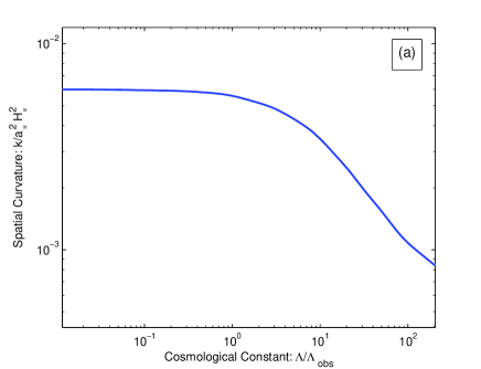
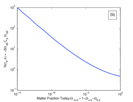
Figure 2: (a) The relationship between the value of the spatial curvature $k$ and the value of $\Lambda$ that dominants the classical history. We show $k$ in units of $a_{\star}^{2}H_{\star}^{2}$ where $1/(a_{\star}H_{\star})$ is a fixed comoving length scale that is equal to $1/(a_{0}H_{0})$ for the observed value of $\Lambda$. $\Lambda$ is shown relative to the value of $\Lambda$ that we observed, $\Lambda_{\rm obs}$. Here the $k-\Lambda$ relationship predicted by our model is for observations at a time $t=t_{\rm U}\approx 13.77\,{\rm Gyrs}$. We have also fixed the $\Lambda$ independent properties of matter by fixing the matter energy per photon, $\xi$, and the baryon energy per photon, $\xi_{\rm b}$, to their observed values: $\xi=3.43\,{\rm eV}$, $\xi_{\rm b}=0.54\,{\rm eV}$. We note that smaller values of $k$ correspond to larger values of $\Lambda$. (b) The relationship between $\Omega_{\rm m0}\approx 1-\Omega_{\rm\Lambda 0}$ and $-2\Omega_{\rm k0}/\zeta_{\rm b}\Omega_{\rm b0}=\mathcal{N}(\tau_{0};\Lambda)$ predicted by our model. When $\Omega_{\rm m0}\approx 1-\Omega_{\rm\Lambda 0}$, we find that when $\mathcal{N}(\tau_{0};\Lambda)$ is expressed as a function of $\Omega_{\rm\Lambda 0}$, it is almost independent of the observation time determined by $\tau_{0}$. For fixed $\Omega_{\rm b0}/\Omega_{\rm m0}$ and $\zeta_{\rm b}$, $\Omega_{\rm k0}$ corresponds to a specific value of $\Omega_{\rm\Lambda 0}$ independently of $\tau_{0}$. As in (a), we have taken $\xi=3.43\,{\rm eV}$, $\xi_{\rm b}=0.54\,{\rm eV}$.

The most recent 1$\sigma$ limit on $\Omega_{k0}$ from WMAP 7 combined with BAO and $H_{0}$ data (and $\Lambda$CDM prior) is Komatsu:2010fb :

$$\Omega_{k0}=-0.0023_{-0.0056}^{+0.0054}.$$ (27)

When our model is applied to our universe with $\Omega_{\Lambda 0}=\Lambda/3H_{0}^{2}=0.73$, $\Omega_{\mathrm{b0}}=0.0423$, as observed at a present time when the CMB temperature is $2.725\,\mathrm{k}$, Eq. (26) predicts the value of $\Omega_{k0}$ to be:

$$\Omega_{k0}=-0.0056\left(\frac{\zeta_{\mathrm{b}}}{1/2}\right)$$ , (28)

which is consistent with the observational limit at 1$\sigma$ for $\zeta_{\mathrm{b}}\in(0,0.7]$ and within the $95\%$ confidence limit for all $\zeta_{\mathrm{b}}\in(0,1]$. For the estimated value of $\zeta_{\mathrm{b}}=1/2$, our model predicts $\Omega_{k0}=-0.0056$. The combination of data from the Planck CMB survey with current and future measurements of the Baryon Acoustic Oscillations (BAO) should be able to confirm or refute this detailed prediction. Therefore, in contrast to other proposals for solving the CC problems, our model makes a testable prediction and is falsifiable in the near future.

III.3 What is a Natural Value of $\Lambda$?

We have seen that, at a fixed time, our model predicts the value of $\Lambda$ in terms the spatial curvature $k$. In inflationary models, the magnitude of spatial curvature $k$ inside the past light cone is determined by the duration of the inflationary period in the earlier universe, specified by the number of e-folds $N$. In most inflationary scenario one imagines that there are many different inflating regions, or “bubble universes”. In each bubble the initial conditions for the scalar field will differ. The number of e-folds of inflation experienced by a bubble universe depends on these initial conditions in a model-dependent fashion. The value of $N$ (and hence $k)$ will therefore be different in each bubble universe. The curvature parameter $k$ is therefore an environmentally sensitive parameter: it depends on the part of universe we observe, and will not be the same everywhere. In our model, when all other quantities are fixed, $\Lambda$ is given implicitly as a function or $k$ by Eq. (26). Hence, the value of $\Lambda$ that one observes at a given time is also an environmentally determined parameter. If we existed in a different bubble universe with a different value of $k$, we would observe a different value of $\Lambda$. In order for our model to be said to solve the CC problems, the value of $\Lambda$ that we do observe must be shown to be in some sense ’natural’. This means that, once selection effects such as the requirement that $\Lambda$ and $k$ are not so large as to prevent the formation of non-linear structure in the universe have been taken into account, the observed value of $\Lambda$ should, ideally, be typical amongst all possible bubble universes. One could then conclude that the observable universe is no more fine tuned that it must be given that we are here to observe it.

Table 1: $\Lambda$ in the history seen by an observer at time $t_{\mathrm{U}}\approx 13.77\,\mathrm{Gyrs}$ for different values of the spatial curvature parameter, $k$. Here, $\zeta_{\mathrm{b}}$ is a QCD constant related to baryon structure, and we expect $\zeta_{\mathrm{b}}\approx 1/2$; $\Lambda_{\mathrm{obs}}$ is the particular value of $\Lambda$ we observe, and $a_{\star}H_{\star}$ is the value of $a(\tau)H(\tau)$ today in our visible universe. We have taken the matter energy per photon to be $\xi=3.43\,\mathrm{eV}$, and the baryon energy per photon is $\xi_{\mathrm{b}}=0.54\,\mathrm{eV}$.

$\frac{k}{2\zeta_{\mathrm{b}}a_{\star}^{2}H_{\star}^{2}}$	$\frac{\Lambda}{\Lambda_{\mathrm{obs}}}$	$\frac{k}{2\zeta_{\mathrm{b}}a_{\star}^{2}H_{\star}^{2}}$	$\frac{\Lambda}{\Lambda_{\mathrm{obs}}}$
0.0060	0.00	0.0049	2.9
0.0059	0.25	0.0042	5.5
0.0057	0.78	0.0034	10.6
0.0056	1.0	0.0018	35.7
0.0053	1.6	0.00084	200

Observers like ourselves require the universe to be old enough for a sufficient number of collapsed structures such as galaxies to have formed, and then for heavy elements to have been formed by stars. If $k$ or $\Lambda$ are too large then either the universe will recollapse before these conditions have been achieved or the growth of structure will have been so suppressed that even as $t\rightarrow\infty$, galaxies never form btip .

III.3.1 The naturalness of $\Lambda$ in string landscape models

Before addressing the naturalness of the observed value of $\Lambda$ in our model, we consider the extent to which the string landscape model solves the CC problems. The string landscape solution to the cosmological constant problems is totally reliant on anthropic selection effects to determine the value of $\Lambda$. In that scenario, it is assumed that there are many different possible vacua, each with a different value of vacuum energy, or equivalently of $\Lambda$. The probability of a vacuum having a CC in the interval $[\Lambda,\Lambda+\,\mathrm{d}\Lambda]$ is $f_{\mathrm{prior}}(\Lambda)\,\mathrm{d}\Lambda$, where $f_{\mathrm{prior}}(\Lambda)$ is the prior probability distribution of $\Lambda$ and has not been directly determined by theory. Anthropic selection effects provide the probability, $f_{\mathrm{selec}}(\Lambda)$, of being able to observe a universe with a given value of $\Lambda$. By Bayes’ theorem, the unnormalized probability distribution function of observing a vacuum state with a CC in the interval $[\Lambda,\Lambda+\,\mathrm{d}\Lambda]$ is:

$$f_{\Lambda}(\Lambda)\,\mathrm{d}\Lambda=f_{\mathrm{selec}}(\Lambda)f_{\mathrm{prior}}(\Lambda)\,\mathrm{d}\Lambda.$$

The form of $f_{\mathrm{selec}}(\Lambda)$ can be estimated by taking the number of galaxies (collapsed structures with a given mass) as a proxy for the number of observers, see for instance Ref. Tegmark:2005dy for such a calculation. However, without knowing the form of $f_{\mathrm{prior}}(\Lambda),$ it is not possible to say whether or not the observed value of $\Lambda$ is natural. Some authors argue that a uniform prior is the most reasonable for small values of $\Lambda$. If this is the case then, as shown in Ref. Tegmark:2005dy , when all other parameters are fixed, the observed value of $\Lambda$ is not atypical, although the most probable values are still an order of magnitude or two larger. Specifically, with a uniform prior, and $f_{\mathrm{selec}}$ from Ref. Tegmark:2005dy , one finds

$$2.84 < \frac{\Lambda}{\Lambda_{\mathrm{obs}}}<44.63,\qquad\text{(68\% Confidence)},$$ (29)

$$0.40 < \frac{\Lambda}{\Lambda_{\mathrm{obs}}}<123.68,\qquad\text{(95\% Confidence)},$$

where $\Lambda_{\mathrm{obs}}$ is the particular value of $\Lambda$ that we observe. Hence, with a uniform prior, this value is outside the 68% confidence limit by about a factor of 2.8 but inside the 95% confidence interval. The observed value of $\Lambda$ is therefore small but not atypically small here.

A uniform prior is not, however, the only reasonable choice one could make for $f_{\mathrm{prior}}(\Lambda)$. A log-prior, $f_{\mathrm{prior}}\,\mathrm{d}\Lambda\propto\,\mathrm{d}\ln\Lambda,$ or an exponential, $f_{\mathrm{prior}}\propto\exp(3\pi/G\Lambda),$ have also be supported by theoretical arguments and in both cases the most probable values of $\Lambda$ would be many orders of magnitude smaller than the observed value. In the string landscape and other multiverse models, the natural value of $\Lambda$ is crucially dependent on the choice of prior, and until the prior can be calculated from first principles using the theory it is not clear whether this model provides an natural explanation for the observed value of $\Lambda$.

III.3.2 The naturalness of $\Lambda$ in our model

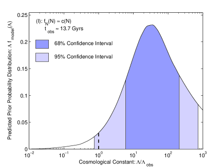
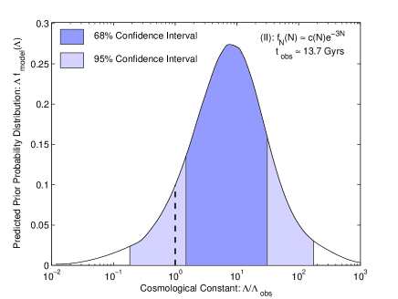
Figure 3: Our model’s prediction for the (prior) probability distribution, $f_{\mathrm{model}}(\Lambda)$, for the value of cosmological constant $\Lambda$ that one would measure at an observation time $t=t_{\mathrm{U}}=13.77\,\mathrm{Gyrs}$. In our theory, the observed value of $\Lambda$ is given as a function of the spatial curvature, $k$, inside the observer’s past light cone. The curvature parameter $k$ depends on $N$, the number of e-folds of inflation. Hence, ultimately, the probability of astronomers observing a given value of $\Lambda$ depends on the prior probability of living in a bubble universe where the universe underwent $N$ e-folds of inflation. The probability distribution function of $N$ is $f_{\mathrm{N}}(N)$. Given an $f_{\mathrm{N}}(N),$ our model completely determines the prior probability distribution function, $f_{\rm model}(\Lambda)$. We have plotted $f_{\rm model}(\Lambda)$ for two different choices of $f_{\mathrm{N}}(N)$. Case I is where $f_{\mathrm{N}}(N)=c(N)$ where $c(N)\approx{\rm const}$ for changes, $\Delta N$, in $N$ over less than $\approx 2.5\%$ (e.g. a power-law $N^{-p}$ for $|p|<10$). Case II is where $f_{\mathrm{N}}=c(N)e^{-3N}$ where again $c(N)\approx{\rm const}$ for $\Delta N/N\lesssim 2.5\%$. This latter choice is the one calculated in Ref. Gibbons:2006pa for slow-roll single-field inflation. In our model this prediction for the prior probability is independent of the fundamental prior weighting of different values of $\Lambda$ in the partition function. Our $f_{\mathrm{model}}(\Lambda)$ does not include any observer-dependent selection effects, apart from the requirement that a classical solution exists. The observed value of $\Lambda$ is shown by a dotted black line, and the whole shaded region is the symmetric 95% confidence interval. The darker shaded area is the symmetric 68% confidence interval. In Case I we have calculated the confidence intervals by sharply cutting off $f_{\rm model}$ for $\Lambda>10^{3}\Lambda_{\rm obs}$, since such large values of the CC are incompatible with the existence of galaxies. For $\Lambda<10^{3}\Lambda_{\rm obs}$ we have not included any weighting by probability of living in a universe with a given $\Lambda$. For these natural choices of $f_{\mathrm{N}}(N)$, the observed value of $\Lambda$ is within the 95% confidence interval in both cases, and well within it for $f_{\rm N}=c(N)e^{-3N}$. In both cases, $\Lambda=\Lambda_{\rm obs}$ is not atypical whatever precise form of the observer conditioned selection effect parametrized by $f_{\rm selec}(\Lambda)$. When selection effects are included the probability of larger values $\Lambda\gtrsim 100\Lambda_{\mathrm{obs}}$ is further suppressed, and the observed value moves within the 1-$\sigma$ confidence interval for Case II, and just outside this interval in Case I. This is shown in FIG 4 below. We have taken the matter energy per photon to be $\xi=3.43\,\mathrm{eV}$, and the baryon energy per photon is $\xi_{\mathrm{b}}=0.54\,\mathrm{eV}$, as is observed.

In our model, we shall see below that, just as in landscape and other multiverse models, anthropic selection still plays a role in limiting the maximum allowed values of $\Lambda$. The equivalent prior on $\Lambda$ in our model is the undetermined measure $\mu[\Lambda]$ in the partition function. Unlike for landscape or multiverse models though, this unknown prior on $\Lambda$ plays no role. This is because our model requires $\Lambda=\Lambda_{0}(k)$ and $\Lambda_{0}(k)$ is a function of $k$ that is given by our model. Thus, whatever the prior on $\Lambda$, the normalized posterior probability distribution of $\Lambda$ given $k$ is a delta-function,

$$f_{\Lambda|k}(\Lambda;k)=\delta(\Lambda-\Lambda_{0}(k)),$$

where $\Lambda_{0}(k)$ also depends on the size of the observer’s past light cone, $\mathcal{M}$, and hence observation time. Given that one lives in a bubble universe with a certain value of $k,$ and observes it at a given time, in our model there is only one value that $\Lambda$ can take. The probability of measuring a $\Lambda$ in a given range is then given entirely by the probability of measuring $k$ in a corresponding range. It is independent of the measure, or prior, $\mu[\Lambda]$.

Now the curvature parameter $k$ is related to the number of e-folds $N$, since $k=k(N)=\bar{k}e^{2(\bar{N}-N)}$ for some fixed $N_{0}$ and $\bar{k}$. As above, $1/(a_{\star}H_{\star})$ is a comoving length scale equal to $1/a_{0}H_{0}$ in our particular universe. In the expression for $k(N)$, $\bar{N}$ is the number of e-folds required to bring about the bound $|\Omega_{\mathrm{k}}|<|\bar{k}|/H_{\star}^{2}a_{\star}^{2}$ today. We are free to take $|\bar{k}|=10^{-2}a_{\star}^{2}H_{\star}^{2}$. Depending on the efficiency of reheating after the end of inflation, we have $\bar{N}\gtrsim 50-62$ in realistic inflation models.

The probability distribution for $k$ in different bubble universes, $f_{k}(k)\,\mathrm{d}k$, is therefore given by $f_{N}(N)\,\mathrm{d}N$, the probability distribution of the number of e-folds, $N$. Specifically, we have

$$f_{k}(k(N))=f_{N}(N)\left|\frac{\,\mathrm{d}N}{\,\mathrm{d}k}\right|=\frac{f_{N}(N(k))}{2k}.$$

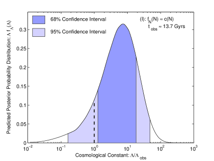
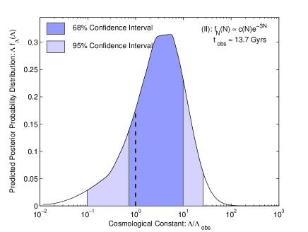
Figure 4: The predicted posterior probability distribution, $f_{\Lambda}(\Lambda)=f_{\rm selec}(\Lambda)f_{\rm model}(\Lambda),$ for the value of cosmological $\Lambda$ that one would measure at an observation time $t=t_{\mathrm{U}}=13.77\,\mathrm{Gyrs}$. Here, $\Lambda_{\mathrm{obs}}$ is the particular value of $\Lambda$ that we have observed. In our theory, the observed value of $\Lambda$ is given as a function of the spatial curvature, $k$, inside the observer’s past light cone. The curvature parameter $k$ depends on $N$, the number of e-folds of inflation. Hence, ultimately, the probability of astronomers observing a given value of $\Lambda$ depends on the prior probability of living in a bubble universe where the universe underwent $N$ e-folds of inflation. The probability distribution function of $N$ is $f_{\mathrm{N}}(N)$. Given an $f_{\mathrm{N}}(N),$ our model completely determines the probability distribution function, $f_{\rm model}(\Lambda)$, of $\Lambda$ prior to the inclusion of selection effects. In the above plots we have included the limits on $\Lambda$ due to observational selection effects using the prescription for $f_{\rm selec}$ given by Tegmark et al. in Tegmark:2005dy which uses the number of galaxies as a proxy for the number of observers. When these are included, the full posterior probability of living in a bubble universe where one observes a given value of $\Lambda$ is $f_{\Lambda}(\Lambda)$. Additionally, we find that the inclusion of selection effects makes $f_{\Lambda}(\Lambda)$ only relatively weakly dependent on the form of $f_{\mathrm{N}}(N)$ because for allowed values of $\Lambda$, the required $k$ (and hence $N$) vary only over a small range. We have plotted $f_{\Lambda}(\Lambda)$ for two different choices of $f_{\mathrm{N}}(N)$. Case I is where $f_{\mathrm{N}}(N)=c(N)$ where $c(N)\approx{\rm const}$ for changes, $\Delta N$, in $N$ over less than $\approx 2.5\%$ (e.g. a power-law $N^{-p}$ for $|p|<10$). Case II is where $f_{\mathrm{N}}=c(N)e^{-3N}$ where again $c(N)\approx{\rm const}$ for $\Delta N/N\lesssim 2.5\%$. This latter choice is the one calculated in Ref. Gibbons:2006pa for slow-roll single-field inflation. In both cases we see that the observed value of $\Lambda$ (dotted black line) is well inside the 95% confidence interval (the shaded areas), and near the boundary of the 68% confidence interval (the more darkly shaded area). In Case I, $\Lambda=\Lambda_{\mathrm{obs}}$ is just outside this interval, whereas in Case II it is just inside it. In both cases, it is clear that the observed value of $\Lambda$ is typical and can be explained without the need for fine tuning. We have taken the matter energy per photon to be $\xi=3.43\,\mathrm{eV}$, and the baryon energy per photon is $\xi_{\mathrm{b}}=0.54\,\mathrm{eV}$ for all values of $\Lambda$.

The calculation of $f_{N}(N)\,\mathrm{d}N$, that is of the probability that the number of e-folds lies in the region $[N,N+\,\mathrm{d}N]$ is the measure problem for inflation, and has been the subject of a considerable amount of work and debate as to which is the correct measure. Recently, Gibbons and Turok Gibbons:2006pa used the natural canonical measure on the space of all classical universes, provided by the Hamiltonian of general relativity Gibbons:1986xk , to show that in single-field, slow-roll inflation, $f_{N}(N)=c(N)e^{-3N}$, where $c(N)$ is model dependent but generally changes much more slowly with $N$ than $\exp(-3N)$. The $\exp(-3N)$ suppression indicates that the region of phase space that results in a long-lived period of slow-roll inflation is very small (however, the result is to some extent just an artefact of having no high-energy cut-off where the theory inevitably breaks down). To find this $f_{\mathrm{N}}$, Gibbons and Turok (GT) have to regularize the canonical measure by imposing a cut-off on the curvature and the end of inflation or equivalently on the scale factor at the end of inflation i.e. $a<a_{\mathrm{max}}$. The regularized measure is then $\propto a_{\mathrm{max}}^{3}$. If one takes $a_{\mathrm{max}}$ to be independent of $N$, then it drops out of the normalized probability distribution for $N$, and $f_{\mathrm{N}}(N)\propto e^{-3N}$. An alternative procedure would be to place the cut-off on the curvature at the beginning of inflation or, equivalently, on the scale-factor there. In this case, at the end of inflation, $a<a_{\mathrm{max}}\propto e^{N}$. We would then have $f_{\mathrm{N}}\rightarrow e^{3N}f_{\mathrm{N}}(N),$ and so $f_{\mathrm{N}}=c(N)$. This procedure factors in a weighting by volume. Another example where $f_{\mathrm{N}}=c(N)$ and $c(N)$ varys much more slowly with $N$ than $\exp(-3N)$ was estimated by Freivogel, Kleban, Rodriguez Martinez, and Susskind (FKRMS), and then extended by De Simone and Salem in the context of eternal inflationary models on the string landscape Freivogel:2005vv ; DeSimone:2009dq . They found $f_{\mathrm{N}}\propto N^{-4}$.

Our model unambiguously predicts the prior probability of living in a universe with effective CC in the interval $[\Lambda,\Lambda+\,\mathrm{d}\Lambda]$. We define this to be $f_{\mathrm{model}}(\Lambda)\,\mathrm{d}\Lambda$, and it is given (up to a calculable normalization factor) by

$$f_{\mathrm{model}}(\Lambda) = \int\,\mathrm{d}k\,f_{\Lambda|k}(\Lambda;k)f_{k}(k),$$

$$= \frac{f_{\mathrm{N}}(N(k_{0}(\Lambda)))}{2}\left|\frac{\,\mathrm{d}\ln k_{0}(\Lambda)}{\,\mathrm{d}\Lambda}\right|,$$

where $k_{0}(\Lambda)$ follows from Eq. (26). Note that $k_{0}(\Lambda)$ also depends on the observation time, and the matter/baryon energy per photon. Depending on the form of $f_{\mathrm{N}}(N)$, the prediction for $f_{\mathrm{model}}(\Lambda)$ may indicate that the observed value of $\Lambda$ is natural independently of selection effects conditioned on the existence of observers. We discuss this point below.

The dependence on the precise form of $f_{\mathrm{N}}(N)$ is greatly weakened when selection effects on $\Lambda$ are included. Then, we have that, in our model, the (unnormalised) posterior probability of living in a universe with effective CC in the interval $[\Lambda,\Lambda+\,\mathrm{d}\Lambda]$ is $f_{\Lambda}(\Lambda)\,\mathrm{d}\Lambda,$ where

$$f_{\Lambda}(\Lambda)=f_{\mathrm{selec}}(\Lambda)f_{\mathrm{model}}(\Lambda).$$

Roughly, the observer-conditioned selection effects on $\Lambda$ limit its value to be no more than about $1000$ times that which is observed in our universe ($\Lambda_{\mathrm{obs}}$). Tegmark et al. Tegmark:2005dy calculated $f_{\mathrm{selec}}(\Lambda)$ by using the number of galaxies (virialized halos with a mass $\gtrsim 10^{12}\,M_{\odot}$) as a proxy for the number of observers. We use their form of $f_{\mathrm{selec}}$ here when evaluating $f_{\Lambda}(\Lambda)$.

Unlike in the string landscape model, $f_{\Lambda}(\Lambda)$ and $f_{\mathrm{model}}(\Lambda)$ have no dependence on the unknown prior weighting of different values of $\Lambda$. All that is required in order to specify $f_{\Lambda}(\Lambda),$ or $f_{\mathrm{model}}(\Lambda),$ fully is to specify the prior probability of the number of e-folds, $f_{\mathrm{N}}(N)$. At present, much more is known and and is calculable about the form of $f_{\mathrm{N}}(N)$ for different inflation models than is known about the landscape prior on $\Lambda$. Also, we shall see that $f_{\Lambda}(\Lambda)$ is much less sensitive to the precise form of $f_{\mathrm{N}}(N)$ than the string landscape model is to $\Lambda$-prior.

In Table 1 we provide the value of $k$ (in units of $H_{\star}^{2}a_{\star}^{2}$) required by our model for different values of $\Lambda$ at an observational time of $13.77\,\mathrm{Gyrs}$. Larger values of $\Lambda$ require a smaller value of $k,$ and hence a larger value of $N$. Given that $f_{\mathrm{N}}(N)$ is generally estimated to be a decreasing function of $N,$ this means that the probability of larger values of $\Lambda$ will be suppressed relative to smaller values. Anthropic limits on $\Lambda$ imply that it could not have been more than about 1000 times larger the value we observe. In this allowed range the required $k$ for a given $\Lambda$ decreases by less than a factor of $10$. Thus, the required number of e-folds, $N=N_{0}(\Lambda)=N(k_{0}(\Lambda),$ changes by less than $\Delta N\approx\Delta(\ln k)/2\lesssim\ln(10)/2\approx 1.2$. At the same time, $N_{0}(\Lambda)\gtrsim\bar{N}>50-62$ in realistic models, and so $\Delta N/N\lesssim 0.025$. So, unless $|\,\mathrm{d}\ln f_{\mathrm{N}}(N)/\,\mathrm{d}\ln N|\gtrsim 10$ or so, we have $f_{\mathrm{N}}(N)\approx\mathrm{const}$ for anthropically allowed values of $\Lambda$. Such a flat $f_{\mathrm{N}}(N)$ emerges if we weight the GT probability distribution for $N$ (which is $\propto e^{-3N}$) by the bubble universe 3-volume at any given time, (which is $\propto e^{3N}$). We then have $f_{\mathrm{N}}=c(N)$ where $c(N)$ is fairly flat (e.g. $c(N)\propto N^{-1/2}$ if the inflationary potential is $\propto m^{2}\phi^{2}$ Gibbons:2006pa ). The FKRMS estimate of $f_{\mathrm{N}}\propto N^{-4}$ is another example where $f_{\mathrm{N}}$ is fairly flat for $\Delta N/N\ll 1$ Freivogel:2005vv ; DeSimone:2009dq . In both these cases $f_{\mathrm{N}}\approx\mathrm{const}$ for allowed values of $\Lambda$ and so the precise form of $f_{\mathrm{N}}(N)$ is unimportant.

The GT measure on inflationary solutions has $f_{\mathrm{N}}\propto e^{-3N}$ and so $|\,\mathrm{d}\ln f_{N}/\,\mathrm{d}\ln N|3N\gg 10$. Thus, if this measure is correct we should not approximate $f_{\mathrm{N}}$ by a constant. We therefore consider this and the $f_{\mathrm{N}}\approx\mathrm{const}$ cases separately.

We note that if $f_{\mathrm{N}}(N)\propto e^{-3N}$, the suppression of large values of $N,$ and of hence large $\Lambda$ values, is actually sufficient to place the observed value of $\Lambda$ within the 95% confidence interval for $\Lambda$ prior to the inclusion of selection effects. Even if we take $f_{\rm N}=c(N)$, where $c(N)$ is fairly flat, the $\Lambda_{\rm obs}$ is inside 95% confidence interval of the prior probability distribution function for $\Lambda$, when one imposes a sharp cut-off on $\Lambda>10^{3}\Lambda_{\rm obs}$. We illustrate this in FIG. 3 where we have plotted $f_{\mathrm{model}}(\Lambda)$ for an observation time of $t_{\mathrm{U}}=13.77\,\mathrm{Gyrs}$. The entire lighter shaded region is the symmetric 95% confidence interval, and the darker shaded region is the symmetric 68% confidence interval. The dotted black line marks the observed value of the CC, $\Lambda_{\mathrm{obs}}$. We see that even before we have included selection effects which suppress $\Lambda\gg 100\Lambda_{\mathrm{obs}}$ outcomes, the observed value of $\Lambda$ is not atypical with either general form of $f_{\rm N}(N)$. For comparison, in the multiverse or landscape model with a uniform prior and a sharp cut-off on $\Lambda>10^{3}\Lambda_{\rm obs}$, $\Lambda\leq\Lambda_{\rm obs}$ is much less likely and has a probability of only $0.1\%$ prior to the inclusion of selection effects.

Whilst there are anthropic selection effects on $k,$ these are automatically satisfied when $k$ is small enough for a classical solution to exist. The existence of a classical solution is therefore by far the strongest selection effect on $k$. Current observational limits require $-0.084<k/a_{\star}^{2}H_{\star}^{2}<0.0133$ at 95% confidence, where $1/a_{\star}H_{\star}$ is the measured value of the comoving Hubble radius, $r_{H}=1/aH,$ today. All the values of $k$ in Table 1 are well within these limits, and so the existence of a classical solution in our model is sufficient to explain why we must live in a bubble universe where $k$ is within the current observational limits, and hence why our observable universe must have undergone a large number of e-folds of inflation, no matter how unlikely that is a priori.

We now turn our attention to the posterior probability, $f_{\Lambda}(\Lambda)\,\mathrm{d}\Lambda,$ of observing $\Lambda$ in the interval $[\Lambda,\Lambda+\,\mathrm{d}\Lambda]$ in our model. We consider the consequences of two general forms of $f_{\mathrm{N}}(N)$: (I) $f_{\mathrm{N}}(N)=c(N)$ where $c(N)\approx\mathrm{const}$ in the allowed range (i.e. less steep than $\sim N^{-10}$) and (II) $f_{\mathrm{N}}(N)\approx c(N)e^{-3N}$ where again $c(N)\approx\mathrm{const}$ for allowed $\Lambda$ values. Finally, for $f_{\mathrm{selec}}(\Lambda)$ we take the form calculated by Tegmark et al. in Ref. Tegmark:2005dy .

In Case I, with $f_{\mathrm{N}}(N)=c(N)\approx\mathrm{const}$, we have

$$f_{\Lambda}(\Lambda)\,\mathrm{d}\Lambda\propto f_{\mathrm{selec}}(\Lambda)\left|\frac{\,\mathrm{d}\ln k(\Lambda)}{\,\mathrm{d}\Lambda}\,\mathrm{d}\Lambda\right|,$$

and in case II where $f_{\mathrm{N}}(N)\propto c(N)e^{-3N}$

$$f_{\Lambda}(\Lambda)\,\mathrm{d}\Lambda\propto f_{\mathrm{selec}}(\Lambda)k^{3/2}(\Lambda)\left|\frac{\,\mathrm{d}\ln k(\Lambda)}{\,\mathrm{d}\Lambda}\,\mathrm{d}\Lambda\right|.$$

In FIG. 4, we plot $\Lambda f_{\Lambda}(\Lambda)$ against $\ln(\Lambda/\Lambda_{\mathrm{obs}})$ for the two cases given above. We also show the 68% and 95% confidence limits on $\Lambda$ in both cases. In case I, for $f_{\mathrm{N}}(N)=c(N)\approx\mathrm{const}$, these limits are:

$$1.31 < \frac{\Lambda}{\Lambda_{\mathrm{obs}}}<18.37,\qquad\text{(68\% Confidence)},$$ (31)

$$0.19 < \frac{\Lambda}{\Lambda_{\mathrm{obs}}}<48.13,\qquad\text{(95\% Confidence)}.$$

In case II, where $f_{\mathrm{N}}(N)=c(N)\exp(-3N)$, ($c(N)\approx\mathrm{const}$) we have:

$$0.76 < \frac{\Lambda}{\Lambda_{\mathrm{obs}}}<10.03,\qquad\text{(68\% Confidence)},$$ (32)

$$0.11 < \frac{\Lambda}{\Lambda_{\mathrm{obs}}}<26.27,\qquad\text{(95\% Confidence)}.$$

We note that, with the same selection effects, for both choices of $f_{\mathrm{N}}$, our model prefers smaller values of $\Lambda$ than does the string landscape model with a uniform prior.

In both cases, the observed value of $\Lambda$, $\Lambda_{\mathrm{obs}}$, is well within the 95% confidence limit. In case I with a power-law $f_{\mathrm{N}}(N)$, $\Lambda=\Lambda_{\mathrm{obs}}$ is just outside the 68% confidence limit, whereas with $f_{\mathrm{N}}\propto\exp(-3N)$, it is just inside this limit. Thus, whichever form $f_{\mathrm{N}}(N)$ takes, the observed value of $\Lambda$ is typical within our model. Note again that this conclusion is independent of the precise form of $f_{\mathrm{N}}(N)$, and totally independent of the prior weighting of different values of $\lambda$.

III.3.3 The Coincidence Problem

To address the coincidence problem directly we can calculate the probability that the cosmological timescale $t_{\Lambda}=1/\sqrt{\Lambda}$ introduced by the CC correlates with the current age of the universe, $t_{\mathrm{U}}\approx 13.77\,\mathrm{Gyrs}$. We define $r=|\ln(t_{\mathrm{U}}/t_{\Lambda})|$, and take, fairly arbitrarily, $r$ to be our measure of the coincidence in the values of $t_{\Lambda}$ and $t_{\mathrm{U}}$. If $r\ll 1$ there is a strong coincidence in the two times, whereas if $r\gg 1$ there is not. Using $f_{\mathrm{posterior}}(\Lambda)$ as provided by our model, we calculate probabilities of living in an observable universe where, at a time $t_{\mathrm{U}}=13.77\,\mathrm{Gyrs}$, $r<r_{0}$ for different choices of $r_{0}$. We find:

$$P(r=|\ln(t_{\mathrm{U}}/t_{\Lambda})|<\tfrac{1}{2}) = 14\%,$$ (33)

$$P(r<1) = 36\%,\qquad\mathrm{(}f_{\mathrm{N}}=c(N)\mathrm{)},$$

$$P(r<\tfrac{1}{2}) = 22\%,$$ (34)

$$P(r<1) = 53\%,\qquad\mathrm{(}f_{\mathrm{N}}=c(N)e^{-3N}\mathrm{)},$$

where in both $c(N)$ cases, $|\,\mathrm{d}\ln c/\,\mathrm{d}\ln\Lambda|\lesssim 10$. It is clear from these figures that within our model, a coincidence in the values of $t_{\mathrm{U}}$ and $t_{\Lambda}$ is quite typical. If we were to do the same calculation for the landscape model with uniform prior on $\Lambda$, we would find $7.0\%$ and $19.7\%$ respectively for $P(r<1/2)$ and $P(r<1)$. Thus, even if we have uniform prior on $\Lambda$, the probability of $t_{\mathrm{U}}$ and $t_{\Lambda}$ coinciding to within a given factor is smaller in the landscape model than in our proposal.

An alternative quantitative statement of the coincidence problem is the probability of observing $O_{0}<\Omega_{\Lambda 0}<1-O_{0}$ for some $O_{0}$, e.g. for $O_{0}=0.1$ and $O_{0}=0.05$, we find:

$$P(\Omega_{\Lambda 0}\in(0.10,0.90)) = 23\%,$$ (35)

$$P(\Omega_{\Lambda 0}\in(0.05,0.95)) = 31\%,\qquad\mathrm{(}f_{\mathrm{N}}=c(N)\mathrm{)},$$

$$P(\Omega_{\Lambda 0}\in(0.10,0.90)) = 35\%,$$ (36)

$$P(\Omega_{\Lambda 0}\in(0.05,0.95)) = 47\%,\qquad\mathrm{(}f_{\mathrm{N}}=c(N)e^{-3N}\mathrm{)}.$$

For comparison, with the same selection effects and a uniform prior on $\Lambda$, the landscape model gives:

$$P(0.10<\Omega_{\Lambda 0}<0.90) = 11\%$$

$$P(0.05<\Omega_{\Lambda 0}<0.95) = 16\%.$$

Again, the observation of a cosmic coincidence in the values of $t_{\Lambda}$ and $t_{U}$ is not atypical in our model or in the string landscape model with uniform prior. However, it is significantly more likely in the model we have proposed, and our model is independent of the choice of prior for $\Lambda$.

IV Concluding Remarks and Possible Questions

The cosmological constant problem and the related coincidence problem are two of the most important unsolved problems in cosmology, and are also of importance for high-energy physics and the search for a complete theory of quantum gravity. So far, cosmologists have only been able to describe the effects of the cosmological constant by introducing an arbitrary $\Lambda$ term chosen to have the observed value ($\Lambda_{\mathrm{obs}}$), or to model it by a scalar field that evolves so slowly that its (dark) energy density is ‘almost’ a cosmological constant at late times (as in quintessence models). It is known that the existence of galaxies, which one may take as a pre-requisite for atom-based observers such as ourselves, would not be possible if $\Lambda\gtrsim 10^{3}\Lambda_{\mathrm{obs}}$. In the context of a multiverse of different universes, each with a different $\Lambda$, using the anthropic upper limit $\Lambda\lesssim 10^{3}\Lambda_{\mathrm{obs}}$ to explain the observed $\Lambda$ depends heavily on the prior likelihood of finding different values of $\Lambda$ in the multiverse. This prior, $f_{\mathrm{prior}}(\Lambda)\,\mathrm{d}\Lambda$, is the fraction of all universes with a CC in the region $[\Lambda,\Lambda+\,\mathrm{d}\Lambda]$. If, for $\Lambda\lesssim 10^{3}\Lambda_{\mathrm{obs}}$, we have $f_{\mathrm{prior}}(\Lambda)\approx\mathrm{const,}$ then the observed value of $\Lambda$ is not atypical in universes compatible with the anthropic limit. Other plausible forms for the prior include a uniform prior in log-space, $f_{\mathrm{prior}}\propto 1/\Lambda,$ or the form $f_{\mathrm{prior}}\propto\exp(3\pi/G\Lambda)$. In either case, non-zero values of $\Lambda$ would be greatly disfavoured and the observed value of $\Lambda$ highly unnatural. However, until it is clear that a uniform prior is (at least approximately) the form of $f_{\mathrm{prior}}$ predicted by fundamental theory, the multiverse/anthropic explanation of $\Lambda$ remains incomplete. Even if it is correct, the multiverse explanation has not so far made any testable predictions.

We have presented a new proposal for solving the cosmological constant and coincidence problems. Crucially, in contrast to the multiverse explanation, our proposal makes a falsifiable prediction. The essence of our new approach is that the bare cosmological constant $\lambda$ is promoted from a parameter to a field. The minimisation of the action with respect to $\lambda$ then yields an additional field equation, Eq. (1) which determines the value of the effective CC, $\Lambda,$ in the classical history that dominates the partition (wave) function of the universe, $Z$. Our proposal is agnostic about the theory of gravity and the number of space-time dimensions.

In the sense that the cosmological constant is promoted to a field, there is a superficial similarity between our proposal and quintessence models. In the latter, the effective cosmological constant depends on a scalar field, $\phi(x^{\mu})$, and the variation of the action with respect to $\phi$ gives a local second-order differential equation which determines the dynamics of $\phi$ up to a specification of two free functions of initial data. In our proposal, the different values of $\lambda$ are summed over in the partition function of the universe, and hence $\lambda$ is a field rather than parameter, but it is not a local scalar field. Whereas a scalar field, $\phi(x^{\mu}),$ may take a different value at every point in space-time, $\lambda$ is the same at all points in a given classical history. Hence, the additional field equation obtained from the variation of the action with respect to $\lambda$ is not, as in quintessence theories, a local second-order differential equation in $\lambda$ (ie $\phi$), but is instead an integral equation, Eq. (3), where the domain of integration is the same as for the action in the partition function, and is algebraic in $\lambda$. This algebraic property means that there are no initial or boundary data for $\lambda$ to specify (unlike in the quintessence case) and our method makes a unique prediction for the value of $\lambda$ in terms of the universal configuration of gravitational and matter fields.

A specific application of our proposal generically results in a testable prediction. We have taken the action in the wave / partition function, $Z$, of the universe to be defined on some manifold $\mathcal{M}$. A choice of definition for $\mathcal{M}$ (e.g. the causal past of the observer) is required for a specific application of our proposal. Different choices will result in different predictions for the effective CC, $\Lambda$. With a given $\mathcal{M}$, the equation for $\lambda$, Eq. (1) can be viewed as a consistency equation which relates the configuration of metric and matter variables in $\mathcal{M}$ to $\lambda$. Eq. (1) can be viewed as a consistency condition on the configuration of the effective CC, $\Lambda,$ the matter, $\Psi^{a}$, and metric, $g_{\mu\nu}$, fields in $\mathcal{M}$. The consistency condition provided by Eq. (1) will be violated for the vast majority of potential configurations $\left\{g_{\mu\nu},\Psi^{a},\Lambda\right\}$ (even if one demands that $g_{\mu\nu}$, $\Psi^{a}$ obey their respective field equations). If observations determine a set of $\left\{g_{\mu\nu},\Psi^{a},\Lambda\right\}$ for which Eq. (1) is violated then our proposal would be falsified. At the same time, if the observed configuration is consistent with Eq. (3) to within observational limits, then our proposal would, for the time being, have passed an important empirical test and remain a credible solution to the CC problems. In addition, if one has measured $\Lambda$ but not (or at least not fully), the $\left\{g_{\mu\nu},\Psi^{a}\right\},$ then Eq. (1) would require that a certain functional of the undetermined $\left\{g_{\mu\nu},\Psi^{a}\right\}$ vanishes. This would represent a prediction of our model which could be tested and falsified by subsequent observations.

In §II we formally described our proposal in its most general form. In §III, we considered in detail the specific and simple case where $\mathcal{M}$ is taken to be the causal past of the observer. With this choice of $\mathcal{M}$, the partition function, $Z[\mathcal{M}]$, and $\Lambda$ equation, only depend on those parts of the universe to which the observer is causally connected. For a given observer, this choice of $\mathcal{M}$ is well-defined in a coordinate invariant fashion. Using this choice, we found that Eq. (3) for $\Lambda$ reduces to a simple form which, keeping only the dominant terms, requires a balance between the spatial curvature and the contribution of baryonic matter to the matter Lagrangian density, $\mathcal{L}_{\mathrm{matter}}$. We defined $\mathcal{L}_{\mathrm{matter}}=-\zeta_{\mathrm{b}}\rho_{\mathrm{baryon}}$ where $\rho_{\mathrm{baryon}}$ is the density of baryonic matter and $\zeta_{\mathrm{b}}$ is a constant whose value can in principle be calculated from QCD. Using an approximate analytical model for baryon structure (the chiral bag model), we estimated $\zeta_{\mathrm{b}}\approx 1/2$. Given the complexity of modelling baryon structure, we conservatively estimate that $\zeta_{\mathrm{b}}=1/2$ only to within $\pm 30\%$ or so.

We found that Eq. (3) is consistent with the current observable limits on $\Lambda$, the spatial curvature, and other observable properties of our universe. If this application of our theory is correct, then the spatial curvature of our universe must take a particular value. This value depends on $\Omega_{\Lambda 0}=\Lambda/3H_{0}^{2}$, and the matter and baryon energy per photon, $\xi$ and $\xi_{\mathrm{b}}$ respectively as well as the time at which observation take place which can be parametrized, for instance by the age of the universe, $t_{\mathrm{U}}$ or the CMB temperature, $T_{\mathrm{CMB}}$. Taking values of $\Omega_{\Lambda 0}=0.73$, $\xi=3.43\,\mathrm{eV}$ and $\xi_{\mathrm{b}}=0.54\,\mathrm{eV}$ (consistent with observations), we found that the observed dimensionless spatial curvature must be:

$$\Omega_{k0}=-0.0056\left(\frac{\zeta_{\mathrm{b}}}{1/2}\right).$$

For reasonable values of $\zeta_{\mathrm{b}}\sim 1/2$, this is within the current 68% confidence limit $\Omega_{k0}=-0.0023_{-0.0056}^{+0.0054}$ from the combination of WMAP7 CMB data, with BAO and $H_{0}$ measurements. Additionally, the predicted value of $\Omega_{k0}$ should be easily confirmed or ruled out by future measurements of the CMB, $H_{0}$ and baryon acoustic oscillations (BAO). For example, a combination of Planck CMB data with the WFMOS BAO has been estimated to be able to determine $\Omega_{k0}$ to a 1-$\sigma$ accuracy of   about $1.76\times 10^{-3}$ Vardanyan:2009ft . With the addition of BAO data from the Square Kilometre Array (SKA) or something similar, the accuracy could be increased to $5.64\times 10^{-4}$ at 68% confidence Vardanyan:2009ft . This would be more than sufficient to rule out an $\Omega_{k0}$ at the predicted level whatever the precise value of $\zeta_{\mathrm{b}}$. This could conclusively test our model as an explanation of the CC problems in the real universe.

For the time being, our model is consistent with current observations. We also considered the extent to which the observed value of $\Lambda$ is typical within our model, and hence whether or not our model can truly be said to solve the CC problems. We found that in our theory the probability of living in a region of the universe where one observes a given value of $\Lambda$ was independent of the fundamental prior weighting on different values of $\Lambda$: instead, it was completely determined by the probability distribution of the number of e-folds of inflation in the early universe, $f_{\mathrm{N}}(N)$. Larger values of $\Lambda$ require smaller $k$ and hence more e-folds of inflation. However, the difference in the value of $N$ required for $\Lambda=0$ and a CC on the edge of the anthropic upper limit ($\Lambda\sim 10^{3}\Lambda_{\mathrm{obs}}$) is only $\Delta N\lesssim 1.2$. At the same time, for a single value of $\Lambda$ to dominate the partition function, and hence for the universe to behave classically, one requires a fairly small curvature and hence $N\gtrsim 50-62$ (depending on the efficiency of reheating). Thus, the anthropically allowed range of values of $\Lambda$ correspond to a range of e-folds with $N\in[\bar{N},\bar{N}+\Delta N],$ where $\Delta N/\bar{N}\ll 1$. This means that the dependence of the posterior probability distribution for $\Lambda$ depends only fairly weakly on $f_{\mathrm{N}}(N)$.

Unless there is a strong (exponential) preference for a value of $\bar{N}+\Delta N$ over $\bar{N}$ (which would increase the preference for larger $\Lambda$) we found that the observed value of $\Lambda$ is indeed typical within our model. Specifically, the observed value, $\Lambda_{\mathrm{obs}}$, lies close (either just inside or just outside depending on $f_{\mathrm{N}}$) the symmetric 1-$\sigma$ confidence interval for $\Lambda$. We also found that the probability of us observing the cosmological coincidence between the value of $t_{\Lambda}$ and the age of the universe is relatively high ($14-53\%$ depending on how one quantifies what counts as a coincidence).

Our proposal for solving the CC is similar in certain respects to other multiverse models such as the string landscape, when $\Lambda$ takes different values in different vacua/parts of the multiverse. Despite this similarity, it differs from multiverse / landscape models in three crucial respects:

(1) Our model is, unlike multiverse models, independent of the fundamental prior weighting on different values of $\Lambda$;

(2) The preference for small $\Lambda$ is our model does not come wholly from anthropic selection effects as it does in multiverse models. Roughly, the prior probability for different values of $\Lambda$ is uniform for $\Lambda\lesssim O(\mathrm{few})\Lambda_{\mathrm{obs}}$ and approximately uniform in log-space for larger values. This means that the probability of observing a value of $\Lambda\sim O(\Lambda_{\mathrm{obs}})$ is typically higher in our model by a factor of $2-5$;

(3) Our model makes a testable prediction for $\Omega_{k0}$ that can be falsified by upcoming CMB/BAO surveys.

 

We now address some possible questions about our proposal:

1. “What is the equation of state of dark energy in this model?”: The equation of state is exactly $w=-1$ i.e. a pure cosmological constant / vacuum energy. Provided that Eq. (3) has a solution, observers see a classical history with a single constant value of the effective CC $\Lambda$ (as determined by Eq. (3)). Since the $\Lambda$ is observed to be constant, it has an effective pressure, $P_{\Lambda}$, equal in magnitude but opposite in sign to its effective energy density, $\rho_{\Lambda}=\kappa^{-1}\Lambda$ and hence $w\equiv P_{\Lambda}/\rho_{\Lambda}=-1$.

2. “Does the observed effective CC depend the time of observation?”: Yes (but see Q. 3). In §III, we the manifold, $\mathcal{M}$, on which the action was defined to be the causal past of the observer, which clearly depends on the time (and position) of the observer. The observed $\Lambda$ depends on $\mathcal{M}$ and $\partial\mathcal{M}$ through Eq. (3) and hence also depends on the observation time. Crucially, however, $\Lambda$ is not seen to evolve. The classical history that dominates the wave function, $Z[\mathcal{M}]$, has a single constant value of $\Lambda$ throughout the observer’s past, $\mathcal{M}$. Thus all observations are consistent with a single constant $\Lambda$ as given by Eq. (3). The observation time changes, so does the classical history that dominants the parition function. Observers at slightly different times would see slightly different classical histories respectively consistent with slightly different values of $\Lambda$. In this way, our proposal is quite unlike the ‘ever-present lambda’ models ever where $\Lambda$ arises as a random space-time fluctuation and is always inversely proportional to the square root of the space-time 4-volume, so $\Lambda\approx Gt^{-2}$ at time $t$. Everpresent-$\Lambda$ models have severe observational problems everJDB and furthermore are only consistent with $\Lambda\sim 1/t_{\rm U}^{2}$ in $3+1$ dimensions (in D+1 spacetime dimensions $\Lambda\sim t^{-(D+1)/2}_{\rm U}$ in natural units).

3. “Can observers at different times establish that they measure different values of $\Lambda$?”: No (at least not classically). Different values of $\Lambda$ correspond to different classical histories. For an observer at one time to communicate the value of $\Lambda$ that they measure to another observer (or even the same observer) at a later time, and hence reveal that the two values are different, they would have to find a way of sending information from one classical history to another. At the classical level (at least) this is not possible. Classically, an observer will see only a history consistent with the value of $\Lambda,$ equal to $\Lambda_{\star}$ say, for their observation time. This would include seeing reports of / remembering all previous measurements of $\Lambda$ as giving $\Lambda=\Lambda_{\star}$.

4. “How does $\Lambda$ change with observation time for the model presented in §III?”: It decreases as the observation time increases. As the observation time, $t_{o}$ increases, the value of the spatial curvature $k$ that is required (i.e. $k_{0}(\Lambda,t_{o})$) for a given value of $\Lambda$ decreases i.e. $k_{0}(\Lambda,t_{1})>k_{0}(\Lambda,t_{2}>t_{1}),$ so at fixed $\Lambda$, $\left.\partial k_{0}/\partial t_{o}\right|_{\Lambda}<0$. We found that at fixed $t$, $\left.\partial k_{0}/\partial\Lambda\right|_{t}<0$. For a given observer, $k$ is fixed. Thus, defining the observed CC at $t_{o}$ to be $\Lambda(t_{o})$, we must have:

   $$\frac{\,\mathrm{d}k_{0}(\Lambda(t_{o}),t_{o})}{\,\mathrm{d}t_{o}}=0=\frac{\,\mathrm{d}\Lambda(t_{o})}{\,\mathrm{d}t_{o}}\frac{\partial k_{0}}{\partial\Lambda}+\frac{\partial k_{0}}{\partial t_{o}}.$$

   It follows that $\,\mathrm{d}\Lambda(t_{o})/\,\mathrm{d}t_{o}<0$. This also means that at some point in the future, $k$ will be too large for Eq. (3) to admit a classical solution. The universe would then cease to have a dominant classical history. One could view this as in some sense the end of the classical universe.

5. “Does this proposal require the existence of a multiverse / landscape?”: No, not in the sense of an ensemble of “parallel” universes with different physical constants. However our model does not exclude it either. Our model does require that the spatial curvature is different for different causally disconnected observers, a scenario that is naturally realized in the context of inflationary theory. Different bubbles of space-time will undergo different amounts of inflation and hence have a different spatial curvature at the same time, however these different bubble universes are all part of the same universe in the sense that a hypothetical tachyonic astronaut could in principle travel between them.

6. “What role does inflation play in this model?”: Inflation in important in this model in two related ways. Firstly, it makes the spatial curvature a spatially varying quantity which is different in different super-horizon-sized regions, and dependent on the number of e-folds of inflation that took place in each causally connected part of the universe. Provided the whole universe (not just the part we see) is large enough (or infinite) the values of $k$ required for a classical history to dominate the wave function in our model will occur at least somewhere. It seems reasonable to assume that this classicality is a prerequisite for the existence of observers such as ourselves. Provided this is the case, it is immediately clear that we could only ever live in those parts of the universe where the number of e-folds $N,$ and the hence spatial curvature $k,$ lies in the small range we reviewed where classical solutions exist and anthropic upper-bounds on $\Lambda$ hold. Secondly, in our model the prior probability (i.e. prior to the inclusion of the anthropic bounds) of observing a CC in $[\Lambda,\Lambda+\,\mathrm{d}\Lambda]$ is related the probability of a given spatial curvature and hence to the probability of a given number of e-folds of inflation.

7. “If future observations rule out the predicted value of $\Omega_{k0}$ does this rule out this proposal?”: Yes, the application of our scheme given in §III where we take $\mathcal{M}$ to the observer’s causal past would be conclusively ruled out. It may be that one could argue the case for a different choice of $\mathcal{M}$, and find another application consistent with observations but this is not something we have investigated at this time. Certainly the choices we made for the particular application of our proposal in §III seem to be the most simple and natural. The only wiggle room is if the QCD parameter $\zeta_{b}$ is significantly different from 0.5, but the required value would then be determined by observations and could be checked against a detailed QCD calculation of $\zeta_{\rm b}$.

In summary: we have introduced a new approach to solving the cosmological constant and coincidence problems. The bare CC, $\lambda$, or equivalently the minimum of the vacuum energy, is allowed to take many possible values in the wave function, $Z$, of the universe. The value of the effective CC in the classical history that dominates $Z$ is given by a new integral field equation, Eq. (1). Our scheme is agnostic about the theory of gravity and the number of space-time dimensions. We have applied it in its simplest and most natural form to a universe in which gravity is described by GR. The observed classical history will be completely consistent with a non-evolving cosmological constant. In an homogeneous and isotropic model of the universe with realistic matter content we find that the observed value of the effective CC is typical, as is a coincidence between $1/\sqrt{\Lambda}$ and the present age of the universe, $t_{U}$. Unlike explanations of the CC problem that rely only on Bayesian selection in a multiverse, our model in independent of the unknown prior weighting of different $\Lambda$ values, and makes a specific numerical prediction for the observed spatial curvature parameter. Specifically, we should observe $\Omega_{k0}=-0.0056(2\zeta_{\mathrm{b}}),$ where the QCD bag parameter is $\zeta_{b}\simeq 0.5$. This prediction is consistent with current observations but can be tested by Planck/BAO observations in the very near future. In conclusion, we have described a new type of solution of the cosmological constant problems. It is consistent with observation and free of fine-tunings, requires no new forms of dark energy or modifications to the low-energy theory of gravity, and is subject to high-precision test by future observations.

Appendix A Connection with Unimodular Gravity

Central to the paradigm we have proposed for solving the CC problems is the promotion of the bare cosmological constant, $\lambda$, from a fixed parameter to a field. Hence the wave-function (partition function) of the universe is a super-position of all possible values of $\lambda$. This concept is not new, and it has been seen to arise naturally in the study of unimodular gravity (see Refs. Henneaux:1984ji ; Unruh:1988in and references therein).

A.1 Unimodular Gravity

Classically, the field equations of unimodular gravity are equivalent to those of general relativity but with the cosmological constant undetermined. Unimodular gravity was first formulated in a non-covariant fashion in terms of the usual Einstein-Hilbert action for GR (and minimally coupled matter action) but with the degrees of freedom in the metric, $g_{\mu\nu}$, restricted by the constraint $\sqrt{-g}=1$. The total action is the unmodified and, dropping surface terms, for some $\lambda$ is given by:

$$I_{\mathrm{tot}} = \frac{1}{2\kappa}\int_{\mathcal{M}}R(g)\sqrt{-g}\,\mathrm{d}^{4}x-\frac{1}{\kappa}\int_{\mathcal{M}}\lambda\sqrt{-g}\,\mathrm{d}^{4}x$$

$$+\int_{\mathcal{M}}\sqrt{-g}\,\mathrm{d}^{4}x\,\mathcal{L}_{\mathrm{matter}}.$$

Since $\sqrt{-g}$ the second term on the right-hand side (the bare CC term) is just a constant and so does not contribute to the field equations found by requiring $\delta I_{\mathrm{tot}}=0$. Varying this action with respect to the unit modulus metric, $\tilde{g}_{\mu\nu}=(-g)^{-1/4}g_{\mu\nu}$, gives the trace-free part of the usual Einstein equation:

$$R^{\mu\nu}-\frac{1}{4}Rg^{\mu\nu}=\kappa\left[T_{\mathrm{matter}}^{\mu\nu}-\frac{1}{4}g^{\mu\nu}T_{\mathrm{matter}}\right].$$

Using $\nabla_{\mu}T_{\mathrm{matter}}^{\mu\nu}=0$ and $\nabla_{\mu}R^{\mu\nu}=\nabla^{\nu}R/2$ we have

$$\nabla^{\mu}(R+\kappa T_{\mathrm{matter}})=0\rightarrow R=-\kappa T_{\mathrm{matter}}+4\Lambda,$$

where $\Lambda=\mathrm{const}$ is a constant of integration. Using the above equation, we then recover the usual Einstein equation with effective cosmological constant $\Lambda$:

$$R^{\mu\nu}-\frac{1}{2}Rg^{\mu\nu}=\kappa T_{\mathrm{matter}}^{\mu\nu}-\Lambda g^{\mu\nu}.$$

In this formulation of unimodular gravity, there is no connection between the effective CC, $\Lambda$, and either the bare cosmological constant $\lambda$ or the vacuum energy from matter $\rho_{\mathrm{vac}}$. Since $\sqrt{-g}=1$, it follows that in unimodular gravity the 4-volume, $V_{\mathcal{M}}$, of $\mathcal{M}$ is fixed where:

$$V_{\mathcal{M}}=\int_{\mathcal{M}}\sqrt{-g}\,\mathrm{d}^{4}x.$$

Fixed $V_{\mathcal{M}}$ is usually taken to be the defining feature of unimodular gravity.

Since $\Lambda$ can take any possible value, the partition/wave function of the universe in unimodular gravity includes a sum over all values of $\Lambda$ with some unspecified weighting $\mu[\Lambda]$:

$$Z_{\mathrm{uni}}=\int\mu[\Lambda]\,\mathrm{d}\Lambda\mathcal{D}g_{\mu\nu}\mathcal{D}\Psi^{a}e^{iI_{\mathrm{tot}}}.$$

Other than the unspecified weight function, $\mu[\Lambda]$, another issue with the original formulation of unimodular gravity is that the constraint $\sqrt{-g}=1$ is not diffeomorphism invariant. Henneaux and Teitelboim Henneaux:1984ji found an action for unimodular gravity that is both diffeomorphism invariant and has the shift symmetry under $\Lambda\rightarrow\Lambda+\mathrm{const}$ which fixes $\mu[\Lambda]=\mathrm{const}$.

The Henneaux-Teitelboim action is

$$I_{\mathrm{HT}}\equiv I_{\mathrm{grav}}+I_{\mathrm{m}}-\frac{1}{\kappa}\int_{\mathcal{M}}\lambda\left(\sqrt{-g}-\partial_{\mu}\tilde{v}^{\mu}\right)\,\mathrm{d}^{4}x,$$

where $I_{\mathrm{grav}}$ is the Einstein-Hilbert action for gravity plus surface terms, $I_{\mathrm{m}}$ is the matter action including the contribution from the vacuum energy; $\tilde{v}^{\mu}$ is a vector-density field and $\lambda=\lambda(x^{\mu})$ is a scalar field. In this formulation $\sqrt{-g}$ is not fixed a priori. However, varying the action with respect to the scalar field $\lambda$ gives $\sqrt{-g}\equiv\partial_{\mu}\tilde{v}^{\mu}$. It follows that there is a shift symmetry under $\lambda\rightarrow\lambda+\delta\lambda$ for constant $\delta\lambda$

$$I_{\mathrm{HT}}\rightarrow I_{\mathrm{HT}}-\frac{\delta\lambda}{\kappa}\int_{\mathcal{M}}\left(\sqrt{-g}-\partial_{\mu}\tilde{v}^{\mu}\right)=I_{\mathrm{HT}},$$

where the last equality comes from $\sqrt{-g}=\nabla_{\mu}\tilde{v}^{\mu}$. Varying the action with respect to $\tilde{v}^{\mu}$ gives:

$$\delta I_{\mathrm{HT}}=\frac{1}{\kappa}\int_{\mathcal{M}}\left[\tilde{v}^{\mu}\partial_{\mu}\lambda+\partial_{\mu}\left(\lambda\delta\tilde{v}^{\mu}\right)\right].$$

For the $\partial_{\mu}(\lambda\delta\tilde{v}^{\mu})$ term to vanish, we must have $\delta\tilde{v}^{\mu}n_{\mu}=0$ on $\partial\mathcal{M}$, where $\partial\mathcal{M}$ corresponds to $f(x^{\mu})=0$ and $n_{\mu}\propto\nabla_{\mu}f$. With $\delta\tilde{v}^{\mu}$ so fixed on $\partial\mathcal{M}$, $\delta I_{\mathrm{HT}}/\delta\tilde{v}^{\mu}=0$ gives

$$\partial_{\mu}\lambda=0\Rightarrow\lambda=\mathrm{const},$$

and so $\lambda$, which represents the bare cosmological constant, is an arbitrary space-time constant. Varying the action with respect to $g_{\mu\nu}$ and requiring that any surface integrals vanish on $\partial\mathcal{M}$, gives

$$R^{\mu\nu}-\frac{1}{2}Rg^{\mu\nu}=\kappa T_{\mathrm{m}}^{\mu\nu}-\lambda g^{\mu\nu}=\kappa T_{\mathrm{matter}}^{\mu\nu}-\Lambda g^{\mu\nu},$$

where $T_{\mathrm{m}}^{\mu\nu}=T_{\mathrm{matter}}^{\mu\nu}-\rho_{\mathrm{vac}}g^{\mu\nu}$ and $\Lambda=\lambda+\kappa\rho_{\mathrm{vac}}$ is the effective CC. Since $\sqrt{-g}=\partial_{\mu}\tilde{v}^{\mu}$, requiring $n_{\mu}\delta\tilde{v}^{\mu}=0$ fixes the four-volume, $V_{\mathcal{M}}$, and ensures that the HT action really does describe a unimodular theory of gravity:

$$V_{\mathcal{M}} = \int_{\mathcal{M}}\,\mathrm{d}^{4}x\sqrt{-g}=\int_{\mathcal{M}}\,\mathrm{d}^{4}x\,\partial_{\mu}\tilde{v}^{\mu},$$

$$\delta V_{\mathcal{M}} = \int_{\mathcal{M}}\,\mathrm{d}^{4}x\,\partial_{\mu}\delta\tilde{v}^{\mu}=0.$$

The partition function for the HT unimodular action is:

$$Z_{\mathrm{HT}}=\int\mathcal{D}\lambda\mathcal{D}\tilde{v}^{\mu}\mathcal{D}g_{\mu\nu}\mathcal{D}\Psi^{a}\mu[\Lambda]e^{iI_{\mathrm{HT}}},$$

where the sum over configurations is for $\tilde{v}^{\mu}$ normal to $\partial\mathcal{M}$ and the matter and metric variables are fixed on the boundary.

A.2 An Alternative Formulation of Our Model

Now, with $I_{\mathrm{tot}}=I_{\mathrm{grav}}+I_{\mathrm{m}}+I_{\mathrm{CC}}[\lambda,g_{\mu\nu};\mathcal{M}],$ we define we have $I_{\mathrm{HT}}=I_{\mathrm{tot}}+I_{v}[\lambda,\tilde{v}^{\mu};\mathcal{M}]$ where

$$I_{v} = \frac{1}{\kappa}\int_{\mathcal{M}}\lambda\partial_{\mu}\tilde{v}^{\mu}=-\int_{\mathcal{M}}\,\mathrm{d}^{4}x\,\tilde{v}^{\mu}\partial_{\mu}\lambda$$

$$+\frac{1}{\kappa}\int_{\mathcal{M}}\partial_{\mu}\left(\lambda\tilde{v}^{\mu}\right),$$

$$= I_{\delta}+I_{\mathrm{v-surf}},$$

$$I_{\delta} = -\int_{\mathcal{M}}\,\mathrm{d}^{4}x\,\tilde{v}^{\mu}\partial_{\mu}\lambda,\qquad I_{\mathrm{v-surf}}=\frac{1}{\kappa}\int_{\mathcal{M}}\partial_{\mu}\left(\lambda\tilde{v}^{\mu}\right).$$

Here, $I_{\mathrm{v-surf}}$ is a total derivative and so represents a surface term in the action and $I_{\delta}$ has the property that

$$\int\mathcal{D}\tilde{v}^{\mu}e^{iI_{\delta}}\propto\delta[\partial_{\mu}\lambda],$$

where $\delta[\partial_{\mu}\lambda]$ is a functional $\delta$-function peaked about space-time constant configurations of $\lambda$, and so acts as

$$\int\mathcal{D}\lambda\,\delta[\partial_{\mu}\lambda]A[\lambda,\dots]=\int_{-\infty}^{\infty}\,\mathrm{d}\lambda\,A[\lambda,\dots].$$

It follows that the partition function in our proposal can be rewritten (up to an arbitrary and irrelevant overall constant) as

$$Z[\mathcal{M}] = \int\,\mathrm{d}\lambda\mathcal{D}g_{\mu\nu}\mathcal{D}\Psi^{a}\mu[\Lambda]e^{iI_{\mathrm{tot}}}$$

$$= \int\mathcal{D}\lambda\,\delta[\partial_{\mu}\lambda]\int\mathcal{D}g_{\mu\nu}\mathcal{D}\Psi^{a}\mu[\Lambda]e^{iI_{\mathrm{tot}}},$$

$$= \int\mathcal{D}\lambda\mathcal{D}\tilde{v}^{\mu}\mathcal{D}g_{\mu\nu}\mathcal{D}\Psi^{a}\mu[\Lambda]e^{i(I_{\mathrm{tot}}+I_{\delta}=I_{\mathrm{HT}}-I_{\mathrm{v-surf}})},$$

where in our proposal the sum over configurations is for some fixed set $\left\{Q^{A}\right\}$ of the metric and matter variables fixed on the boundary; $\tilde{v}^{\mu}$ is just a Lagrange multiplier field here and so is not assumed to be fixed anywhere.

It is clear from the second line of Ref. (A.2) that there is an aesthetic similarity between the partition function in our proposal and that in the HT formulation of unimodular gravity. Both theories can be formulated in terms of a scalar field $\lambda(x^{\mu})$ and vector-density $\tilde{v}^{\mu}$ in addition to the usual metric and matter fields. When written in this way, the action in our proposal is $I_{\mathrm{tot}}+I_{\delta}$ with differs from the action in the HT proposal by a surface term $I_{\mathrm{v-surf}}$. The two formulations also differ in terms of what is taken to be fixed on the boundary, with the main difference being that in HT unimodular gravity, $\tilde{v}^{\mu}$ is fixed normal to $\partial\mathcal{M}$, which in turn fixes the 4-volume, $V_{\mathcal{M}}$, of $\mathcal{M}$. In our formulation the addition of the subtraction of the surface term $I_{\mathrm{v-surf}}$ relative to $I_{\mathrm{HT}}$, means that one no longer needs to require $\delta\tilde{v}^{\mu}n_{\mu}=0$ on $\partial\mathcal{M,}$ and hence the $V_{\mathcal{M}}$ is not fixed in our proposal and it is not a unimodular gravity theory, despite its similarities to the HT theory.

Varying the action in our model, produces terms proportional to $\delta\lambda$. Defining $I_{\mathrm{full}}=I_{\mathrm{tot}}+I_{\delta}$, and assuming a GHY surface term for gravity for illustrative purposes

$$\delta I_{\mathrm{full}} = \int_{\mathcal{M}}\,\mathrm{d}^{4}x\left[\frac{1}{2\kappa}\tilde{E}^{\mu\nu}\delta g_{\mu\nu}+\tilde{\Phi}_{a}\delta\Psi^{a}-\kappa^{-1}\delta\tilde{v}^{\mu}\partial_{\mu}\lambda\right.$$

$$\left.-\kappa^{-1}\delta\lambda\left(\sqrt{-g}-\partial_{\mu}\tilde{v}^{\mu}\right)\right]$$

$$+ \int_{\partial\mathcal{M}}\sqrt{|\gamma|}\,\mathrm{d}^{3}x\left[\kappa^{-1}N^{\mu\nu}\delta\gamma_{\mu\nu}+\Sigma_{a}\delta\Psi^{a}\right.$$

$$\left.-\kappa^{-1}\delta\lambda f_{\mu}\tilde{v}^{\mu}\right],$$

where $\partial\mathcal{M}$ corresponds to $f(x^{\mu})=0$, $f<0$ in $\mathcal{M}$, and $f_{\mu}=\nabla_{\mu}f$. Here, $\gamma_{\mu\nu}$ is the induced metric on $\partial\mathcal{M}$, and $\tilde{E}^{\mu\nu}=E^{\mu\nu}=\kappa T_{\mathrm{matter}}^{\mu\nu}-G^{\mu\nu}-\Lambda g^{\mu\nu}$; $\tilde{\Phi}_{a}=\sqrt{-g}\Phi_{a}$ and $\Lambda=\lambda+\rho_{\mathrm{vac}}$ is the effective CC. The classical field equations for $g_{\mu\nu}$ and $\Psi^{a}$ are then $E^{\mu\nu}=\Phi_{a}=0$ and these cause the variation of $I_{\mathrm{full}}$ with respect to $g_{\mu\nu}$ and $\Psi^{a}$ to vanish in the bulk (i.e. in $\mathcal{M}$). Similarly, requiring $\delta I_{\mathrm{full}}=0$ with respect to variations of $\lambda$ and $\tilde{v}^{\mu}$ in the bulk gives:

$$\sqrt{-g}=\partial_{\mu}\tilde{v}^{\mu},\qquad\partial_{\mu}\lambda=0.$$

When these field equations hold in the bulk, $\delta I_{\mathrm{full}}$ reduces to surface integrals over $\partial\mathcal{M}$. Since $\partial_{\mu}\lambda=0$, the allowed variations of $\lambda$ are those for which $\delta\lambda$ is a space-time constant. Hence,

$$\delta I_{\mathrm{full}} = \int_{\partial\mathcal{M}}\,\mathrm{d}^{3}x\sqrt{\gamma}\left[\kappa^{-1}\tilde{N}^{\mu\nu}\delta\gamma_{\mu\nu}+\tilde{\Sigma}_{a}\delta\Psi^{a}\right.$$

$$\left.-\delta\lambda\int_{\partial\mathcal{M}}\,\mathrm{d}^{3}x\,\kappa^{-1}f_{\mu}\tilde{v}^{\mu}\right],$$

$$= \int_{\partial\mathcal{M}}\,\mathrm{d}^{3}x\sqrt{\gamma}\left[\kappa^{-1}\tilde{N}^{\mu\nu}\delta\gamma_{\mu\nu}+\tilde{\Sigma}_{a}\delta\Psi^{a}\right]$$

$$-\delta\lambda\frac{1}{\kappa}\int_{\mathcal{M}}\sqrt{-g}\,\mathrm{d}^{4}x,$$

where in the second line we have used $\sqrt{-g}=\partial_{\mu}\tilde{v}^{\mu}$ to eliminate all appearances of the Lagrange multiplier field $\tilde{v}^{\mu}$.

We wish to have $\delta I_{\mathrm{full}}=0$ for the classical solution. This could be achieved by taking $\delta\gamma_{\mu\nu}=\delta\Psi^{a}=0$ (for all $\lambda$) on $\partial\mathcal{M}$ and $\delta\lambda=0$. Indeed fixing $\gamma_{\mu\nu}$ and $\Psi^{a}$ on $\partial\mathcal{M}$ would, modulo the field equations, generally fix $\lambda$ and set $\delta\lambda=0$. However, fixing $\lambda$ in $\mathcal{M}$ returns us to the usual action of general relativity where the bare CC is some fixed external parameter. Thus, to preserve the nature of $\lambda$ as a configuration variable that is integrated over the partition function, we cannot take either $\delta\lambda=0$ or $\delta\gamma_{\mu\nu}=\delta\Psi^{a}=0$ (for all $\lambda$).

In our scheme for solving the CC problems, we propose making a different ansatz: $\delta\gamma_{\mu\nu}=\mathcal{H}_{\mu\nu}\delta\lambda$ and $\delta\Psi^{a}=\mathcal{P}^{a}\delta\lambda$ where the form of $\mathcal{H}_{\mu\nu}$ and $\mathcal{P}^{a}$ must be consistent with the classical field equations. This is equivalent to fixing $\gamma_{\mu\nu}$ and $\mathcal{P}^{a}$ only for each value of $\lambda$ rather than for all $\lambda$. Then, we have

$$\delta I_{\mathrm{full}} = \delta\lambda\left(\int_{\partial\mathcal{M}}\sqrt{\gamma}\,\mathrm{d}^{3}x\left[\kappa^{-1}N^{\mu\nu}\mathcal{H}_{\mu\nu}+\Sigma_{a}\mathcal{P}^{a}\right]\right.$$

$$\left.-\kappa^{-1}\int_{\partial\mathcal{M}}\,\mathrm{d}^{3}x\,f_{\mu}\tilde{v}^{\mu}\right),$$

and so we can have classical solutions where $\delta I_{\mathrm{full}}=0$ without having to externally fix $\lambda$ (i.e. set $\delta\lambda=0$). Quantum mechanically, $\lambda$ can take all possible values and the partition/wave function is a super-position over histories with all possible values of $\lambda$. Classically, the dominant history is the one where the value of $\lambda$ is such that $\delta I_{\mathrm{full}}=0$ i.e.:

$$\int_{\partial\mathcal{M}}\sqrt{\gamma}\,\mathrm{d}^{3}x\left[\kappa^{-1}N^{\mu\nu}\mathcal{H}_{\mu\nu}+\Sigma_{a}\mathcal{P}^{a}\right] = \frac{1}{\kappa}\int_{\partial\mathcal{M}}\,\mathrm{d}^{3}x\,f_{\mu}\tilde{v}^{\mu}$$

$$= \frac{1}{\kappa}\int_{\mathcal{M}}\sqrt{-g}\,\mathrm{d}^{4}x.$$

In §II.2, we showed that equation of $\Lambda$ in our theory is entirely equivalent to

$$\frac{\,\mathrm{d}I_{\mathrm{class}}}{\,\mathrm{d}\lambda}=0,$$

where $I_{\mathrm{class}}$ is the value of $I_{\mathrm{tot}}$ when the classical field equations hold for the matter and the metric.

Since $\lambda$ only ever appears in the other field equations in the combination $\lambda+\kappa\rho_{\mathrm{vac}}=\Lambda$, this is a field equation for the effective CC, $\Lambda$. We note that by introducing the Lagrange multiplier field $\tilde{v}^{\mu}$, this field equation is equivalent to the vanishing of a surface-integral over the boundary $\partial\mathcal{M}$. In this sense, it can be said to be holographic.

A.3 Summary

In this appendix, we have seen that our proposal can alternatively be formulated in terms of the action $I_{\mathrm{full}}=I_{\mathrm{tot}}+I_{\delta}$ and an ansatz about how the boundary metric and matter fields depend on $\Lambda$ which is required to preserve the freedom to vary the bare cosmological constant $\lambda$.

We noted that $I_{\mathrm{full}}$ is almost equivalent to the Henneaux-Teitelboim action, $I_{\mathrm{HT}}$ for unimodular gravity with the only difference between a surface term, $I_{\mathrm{v-surf}}$. Despite this similarity, the subtraction of $I_{\mathrm{v-surf}}$ from $I_{\mathrm{HT}}$ to $I_{\mathrm{full}}$ greatly alters the properties of the theory as in our model one does not need to fix the four-volume, $V_{\mathcal{M}}$, whereas in the HT model, as a unimodular gravity theory, $V_{\mathcal{M}}$ must be held fixed to return the usual classical field equations. Both unimodular gravity and our proposal feature a sum over all possible values of the bare CC, $\lambda$, in the partition function. This sum includes an unspecified weight, or prior, on $\Lambda$: $\mu[\Lambda]$. In unimodular gravity there is no accompanying classical field equation for $\lambda$ and so it remains completely unspecified. The weighting $\mu[\Lambda]$ then plays an important role in determining the relative contributions of different values of $\lambda$ to the partition function. In our model, the subtraction of a surface term from the unimodular action, combined with the ansatz about the dependence of boundary quantities on $\lambda$, provides a field equation which determines the classical value of the effective CC. The partition function is strongly peaked about the value of $\lambda$ for which this field equation holds. In this classical limit, only this value of $\lambda$ contributes to the partition function and $\mu[\Lambda]$ simply becomes an irrelevant overall constant multiplying the partition function. Its form is no longer important. Physics in our model is independent of the prior weighting function $\mu[\Lambda]$ to an excellent approximation whereas in unimodular gravity it is not. We also saw that the $\Lambda$ equation in our model can be written in a holographic fashion, as the vanishing of an integral over the boundary $\partial\mathcal{M}$.

Appendix B Surfaces Terms in General Relativity

In this appendix we rederive, for completeness, the form of the surface terms which must be added to the usual Einstein-Hilbert action, $I_{\mathrm{EH}}$, to make it first order in derivatives of the metric. The need for these boundary terms was first realized by York York:1972sj , and then rediscovered and refined by Gibbons and Hawking Gibbons:1976ue . York, and then Gibbons and Hawking, explicitly derived the form of the required surface term for a non-null boundary. The equivalent surface terms for null boundaries follow from a double null decomposition of the Einstein field equations, see Refs. Brady:1995na ; Geroch:1973am , although this has rarely been explicitly stated. We detail the derivation of the Gibbons-Hawking-York (GHY) surface terms, $I_{\mathrm{GHY}}$, for a ‘cosmological’ boundary defined to be the union of the surface of past-light cone of a given observer, $\partial\mathcal{M}_{u}$ boundary and some initial hypersurface $\partial\mathcal{M}_{I}$ with timelike normal. For this setting, we explicitly state how the variation of $I_{\mathrm{grav}}=I_{\mathrm{EH}}+I_{\mathrm{GHY}}$ depends on the metric on the boundary. We also restate the definition of York’s cosmological surface term, $I_{\mathrm{YC}}$, defined in Ref. York:1972sj , since this is relevant for boundaries such as the initial singularity.

We take $\mathcal{M}$ to be the manifold where $u(x^{\mu})<0$ and $0<\tau(x^{\mu})<\tau_{0}$ for some $u(x^{\mu})$ and $\tau(x^{\mu})$. We define $u(x^{\mu})=\tau_{0}$ on the past-light of an observer (at $\tau=\tau_{0}$) and $w(x^{\mu})$ to be a null coordinate that lies perpendicular to $u$, defined so that $\tau=(u+w)/2$; $\tau$ is a timelike coordinate i.e. $\nabla_{\mu}\tau\nabla^{\mu}\tau<0$.

An integral over $\mathcal{M}$ is equivalent to an integral over the whole space-time weighted by $H(-u)H(\tau)H(\tau_{0}-\tau)$ where $H(y)$ is the Heaviside function which is unity for $y>0$ and vanishes for $y<0$; $\,\mathrm{d}H(y)/\,\mathrm{d}y=\delta(y)$ where $\delta(y)$ is the Dirac delta function.

We therefore write:

$$\mathcal{M}=\left\{x^{\mu}:H(\tau_{0}-u)H(\tau)H(\tau_{0}-\tau)>0\right\},$$

and $\partial\mathcal{M}=\partial\mathcal{M}_{u}\cup\partial\mathcal{M}_{I}$ where $\partial\mathcal{M}_{u}$ is $\{u=\tau_{0},0<\tau<\tau_{0}\}$ and $\partial\mathcal{M}_{I}$ is $\{u<\tau_{0},\tau=0\}$. We define $u_{\mu}=\nabla_{\mu}u$ and $w_{\mu}=\nabla_{\mu}w$. Now $u$ and $w$ are null coordinates so $u^{\mu}u_{\mu}=w_{\mu}w^{\mu}=0$ and we define $u_{\mu}w^{\mu}=-2e^{-2\sigma}$. We also define $\tau_{\mu}=\nabla_{\mu}\tau$. Since $\tau=(u+w)/2$ it follows that $\tau_{\mu}\tau^{\mu}=-e^{-2\sigma}$. We define $m_{\mu}=e^{\sigma}\tau_{\mu}$ so that $m_{\mu}m^{\mu}=-1$ and then $n_{\mu}=e^{\sigma}u_{\mu}$. We then have $m_{\mu}n^{\mu}=1$. Finally, we define $\{\theta^{i}\}$, $i=1,2$, to be intrinsic coordinates on the surfaces, $S$, of constant $\tau$ and $u$. We define $e_{\mu}^{i}=\partial_{\mu}\theta^{i}$. The metric $g_{\mu\nu}$ can then be decomposed thus:

$$g_{\mu\nu}=n_{\mu}n_{\nu}+2n_{(\nu}m_{\mu)}+h_{\mu\nu},$$ (39)

where $h_{\mu\nu}n^{\mu}=h_{\mu\nu}m^{\mu}=0$.

The Einstein-Hilbert action for General Relativity is:

$$I_{\mathrm{EH}}=\frac{1}{2\kappa}\int_{\mathcal{M}}\sqrt{-g}R(g)\,\mathrm{d}^{4}x,$$

where $R(g)$ is the Ricci scalar curvature of $g_{\mu\nu}$. This is second order in derivatives of the metric.

B.1 GHY Surface Term

On a non-null boundary, the Gibbons-Hawking-York surface term, $I_{\mathrm{GHY}}$, is the surface term that must be added $I_{\mathrm{EH}}$ to make $I_{\mathrm{EH}}+I_{\mathrm{GHY}}$ first order in derivatives of the metric. It is natural to extend this definition to null boundaries, so that on a general boundary $I_{\mathrm{EH}}+I_{\mathrm{GHY}}$ is first order in derivatives of the metric. We use this definition to find the form of $I_{\mathrm{GHY}}$ for our $\partial\mathcal{M}$. This is more simply and clearly done by writing the metric in terms of a vierbein $E_{\mu}^{I}$, $I=1,2,3,4,$ where $g_{\mu\nu}=E_{\mu}^{I}E_{\nu}^{J}\eta_{IJ}$ for some fixed $\eta_{IJ}$; $\mathrm{det}\eta=-1$. We choose a form for $\eta_{IJ}$ suited for a decomposition of the metric along a null and a time-like direction:

$$\eta_{IJ} = \left(\begin{array}[]{cc}\mathbb{I}_{2\times 2}&0\\ 0&\mathbb{N}_{2\times 2}\end{array}\right),\qquad\mathbb{N}_{2\times 2}=\left(\begin{array}[]{cc}1&1\\ 1&0\end{array}\right),$$ (44)

$$\mathbb{I}_{2\times 2} = \mathrm{diag}(1,1).$$

We use $\eta_{IJ}$ and its inverse $\eta^{IJ}$ to raise and lower indices $I$.

It follows from $g_{\mu\nu}=E_{\mu}^{I}E_{\nu}^{J}\eta_{IJ}$ that

$$g_{\mu\nu}=E_{\mu}^{3}E_{\nu}^{3}+2E_{(\mu}^{3}E_{\nu)}^{4}+\sum_{i=1}^{2}E_{\mu}^{i}E_{\nu}^{j}.$$ (45)

Comparing Eqs. (39) and (45), we see that we can take $E_{\mu}^{3}=n_{\mu}$, $E_{\mu}^{4}=m_{\mu}$ and then $h_{\mu\nu}=E_{\mu}^{1}E_{\nu}^{1}+E_{\mu}^{2}E_{\nu}^{2}$. With intrinsic coordinates $\{\theta^{i}\}$ on $\{u,\tau\}=\mathrm{const}$ surfaces, $S$, we have: $E_{\mu}^{i}=a^{i}{}_{j}\left[e_{\mu}^{i}+K^{i}u_{\mu}+\beta^{j}\tau_{\mu}\right]$ and let $h_{ij}=\sum_{l}a^{l}{}_{i}a^{l}{}_{j}$. $h_{ij}$ is then the induced 2-metric on $S$ and $K^{i}$ and $\beta^{i}$ are shift 2-vectors. We also define a ‘radial’ coordinate, $r$, on surfaces of constant $\tau$ by $r=(u-w)/2$.

Thus, we have

$$g_{\mu\nu}\,\mathrm{d}x^{\mu}\,\mathrm{d}x^{\nu} = e^{2\sigma}\,\mathrm{d}u^{2}-2e^{\sigma}N\,\mathrm{d}u\,\mathrm{d}\tau+h_{ij}\mathrm{D}\theta^{i}\mathrm{D}\theta^{j},$$

$$\mathrm{D}\theta^{i} = \mathrm{d}\theta^{i}+K^{i}\,\mathrm{d}u+\beta^{i}\,\mathrm{d}\tau.$$

Now $E^{\mu I}$ is a 4-vector and so

$$R(g) = E^{\nu}{}_{I}\left[\nabla_{\mu},\nabla_{\nu}\right]E^{\mu I}=\nabla_{\mu}\left[E^{\nu}{}_{I}\nabla_{\nu}E^{\mu I}-E^{\mu}{}_{I}\nabla_{\nu}E^{\nu I}\right]$$

$$+\nabla_{\mu}E^{\mu}{}_{I}\nabla_{\nu}E^{\nu I}-\nabla_{\mu}E^{\nu}{}_{I}\nabla_{\nu}E^{\mu I}.$$

We define $\omega^{\mu\nu\rho}=-\omega^{\mu\rho\nu}=E_{I}^{\rho}\nabla^{\mu}E^{\nu I}$. In terms of the vierbein, we can rewrite $I_{\mathrm{EH}}$ in the following form:

$$I_{\mathrm{EH}} = \frac{1}{2\kappa}\int_{\mathcal{M}}\sqrt{-g}\,\mathrm{d}^{4}x\,R(g)=-\frac{1}{\kappa}\int_{\mathcal{M}}\partial_{\rho}\left[\sqrt{-g}\omega_{\mu}{}^{\mu\rho}\right]$$ (46)

$$+\frac{1}{2\kappa}\int_{\mathcal{M}}\sqrt{-g}\,\mathrm{d}^{4}x\,\left[\omega_{\nu}{}^{\nu\rho}\omega^{\mu}{}_{\mu\rho}-\omega^{\mu\nu\rho}\omega_{\nu\mu\rho}\right].$$

All second derivatives of the vierbein, and hence also of the metric, are contained in the term

$$-\frac{1}{\kappa}\int_{\mathcal{M}}\partial_{\rho}\left[\sqrt{-g}\omega_{\mu}{}^{\mu\rho}\right].$$

Since this term is a total derivative it is equivalent to a surface integral over $\partial\mathcal{M}$. $I_{\mathrm{GHY}}$ is the surface term which must be added to the action to remove second derivatives of the metric, it is clear from Eq. (46) that:

$$I_{\mathrm{GHY}} = \frac{1}{\kappa}\int_{\mathcal{M}}\partial_{\rho}\left[\sqrt{-g}\omega_{\mu}{}^{\mu\rho}\right]==I_{\mathrm{GHY}}^{(u)}+I_{\mathrm{GHY}}^{(I)},$$ (47)

$$I_{\mathrm{GHY}}^{(u)} = \frac{1}{\kappa}\int_{\partial\mathcal{M}_{u}}e^{\sigma}\sqrt{h}\,\mathrm{d}\tau\,\mathrm{d}^{2}\theta\,\left[-n_{\rho}\omega_{\mu}{}^{\mu\rho}\right],$$ (48)

$$I_{\mathrm{GHY}}^{(I)} = \frac{1}{\kappa}\int_{\partial\mathcal{M}_{I}}e^{\sigma}\sqrt{h}\,\mathrm{d}r\,\mathrm{d}^{2}\theta\,\left[-m_{\rho}\omega_{\mu}{}^{\mu\rho}\right].$$ (49)

Then, with $G^{\mu\nu}=R^{\mu\nu}-\frac{1}{2}Rg^{\mu\nu}$, varying $I_{\mathrm{EH}}+I_{\mathrm{GHY}}$ with respect to the vierbein gives:

$$\delta(I_{\mathrm{EH}}+I_{\mathrm{GHY}}) = -\frac{1}{2\kappa}\int_{\mathcal{M}}\,\mathrm{d}^{4}x\,\sqrt{-g}G^{\mu\nu}\delta g_{\mu\nu}$$

$$-\frac{1}{2\kappa}\int_{\mathcal{M}}\,\mathrm{d}^{4}x\,\partial_{\rho}\left[\sqrt{-g}S^{\mu\nu\rho}2E_{\nu I}\delta E_{\mu}^{I}\right].$$

where

$$S^{\mu\nu\rho}=\omega^{\nu\mu\rho}-\omega_{\sigma}{}^{\sigma\rho}g^{\mu\nu}+\omega_{\sigma}{}^{\sigma\mu}g^{\nu\rho},$$

We note that $S^{\mu\nu\rho}V_{\mu}V_{\rho}=0$ for any $V_{\mu}$.

We define:

$$\delta I^{(u)}+\delta I^{(I)} = -\frac{1}{2\kappa}\int_{\mathcal{M}}\,\mathrm{d}^{4}x\,\partial_{\rho}\left[\sqrt{-g}S^{\mu\nu\rho}2E_{\nu I}\delta E_{\mu}^{I}\right],$$

$$\delta I^{(u)} = \frac{1}{2\kappa}\int_{\partial\mathcal{M}_{u}}e^{\sigma}\sqrt{h}\,\mathrm{d}\tau\,\mathrm{d}^{2}\theta\,\left[n_{\rho}S^{\mu\nu\rho}2E_{\nu I}\delta E_{\mu}^{I}\right],$$

$$\delta I^{(I)} = \frac{1}{2\kappa}\int_{\partial\mathcal{M}_{I}}e^{\sigma}\sqrt{h}\,\mathrm{d}r\,\mathrm{d}^{2}\theta\,\left[m_{\rho}S^{\mu\nu\rho}2E_{\nu I}\delta E_{\mu}^{I}\right].$$

We now re-express the $I_{\mathrm{GHY}}^{(u)}$, $I_{\mathrm{GHY}}^{(I)}$, $\delta I^{(u)}$ and $\delta I^{(I)}$ in a more familiar form in terms of the geometry of the boundaries $\partial\mathcal{M}_{u}$ and $\partial\mathcal{M}_{I}$. We note that $E_{\rho}^{I}\omega^{\mu\nu\rho}=\nabla^{\mu}E^{\nu I}$ and so

$$-n_{\rho}\omega^{\mu\nu\rho} = -E_{\rho}^{3}\omega^{\mu\nu\rho}=-\nabla^{\mu}n^{\nu},$$

$$-m_{\rho}\omega^{\mu\nu\rho} = -E_{\rho}^{4}\omega^{\mu\nu\rho}=-\nabla^{\mu}m^{\nu}.$$

Null Boundary:

We begin by considering the null boundary, $\partial\mathcal{M}_{u}$, given by $u=0$. We define $\mathcal{K}^{\mu\nu}$ to be the extrinsic curvature of $h_{\mu\nu}$ along $n^{\mu}$:

$$\mathcal{K}^{\mu\nu}=\mathcal{K}^{\nu\mu}=-\frac{1}{2}h^{\mu\rho}h^{\nu\sigma}\mathcal{L}_{n}h_{\rho\sigma}=-h^{\mu\rho}h^{\nu\sigma}\nabla_{\rho}n_{\sigma}.$$

Thus, with $\mathcal{K}=\mathcal{K}^{\mu\nu}g_{\mu\nu}=\mathcal{K}^{\mu\nu}h_{\mu\nu}$ and using $n^{\rho}n_{\rho}=0$,

$$-n_{\rho}\omega_{\mu}{}^{\mu\rho}=-\nabla_{\rho}n^{\rho}=\mathcal{K}-n_{\mu}m_{\nu}\nabla^{\mu}n^{\nu}=\mathcal{K}+\nu,$$

where

$$\nu=-n_{\mu}m_{\nu}\nabla^{\mu}n^{\nu}=-\mathcal{L}_{n}\sigma=-n^{\mu}\nabla_{\mu}\sigma$$

is the in-affinity. Using this, the GHY term on $\partial\mathcal{M}_{u}$ can be written succinctly as:

$$I_{\mathrm{GHY}}^{(u)}=\frac{1}{\kappa}\int_{\partial\mathcal{M}_{u}}e^{\sigma}\sqrt{h}\,\mathrm{d}\tau\,\mathrm{d}^{2}\theta\,\left[\mathcal{K}+\nu\right].$$

We now consider $\delta I^{(u)}$ with $u$ and $\tau$ fixed $\delta E_{\mu}^{3}=\delta n_{\mu}=n_{\mu}\delta\sigma$ and $\delta E_{\mu}^{4}=\delta m_{\mu}=m_{\mu}\delta\sigma$. Using these equations and $S^{\mu\nu\rho}n_{\mu}n_{\rho}=0$

$$n_{\rho}S^{\mu\nu\rho}2E_{\nu I}\delta E_{\mu}^{I}=\sum_{i=1}^{2}n_{\rho}S^{\mu\nu\rho}2E_{\nu i}\delta E_{\mu}^{i}+2n_{\rho}n_{\nu}m_{\mu}S^{\mu\nu\rho}\delta\sigma,$$

and

$$n_{\rho}S^{\mu\nu\rho}=\nabla^{\nu}n^{\mu}-g^{\mu\nu}\nabla_{\rho}n^{\rho}+\omega_{\sigma}^{\sigma\mu}n^{\nu},$$

$h^{\mu\rho}\nabla_{\rho}n^{\nu}$ can be decomposed as

$$h^{\mu\rho}\nabla_{\rho}n^{\nu} = -\mathcal{K}^{\mu\nu}+n^{\nu}m_{\sigma}h^{\mu\rho}\nabla_{\rho}n^{\sigma}$$

$$= -K^{\mu\nu}+n^{\mu}\omega^{\mu},$$

$$\omega^{\mu} = h^{\mu\rho}m_{\sigma}\nabla_{\rho}n^{\sigma},$$

and we define $\mathcal{K}^{ij}=\mathcal{K}^{\mu\nu}e_{\mu}^{i}e_{\nu}^{j}$ and $\omega^{i}=\omega^{\mu}e_{\mu}^{i}$; $\omega_{i}=\omega^{j}h_{ij}$.

Then, we find:

$$n_{\rho}n_{\nu}m_{\mu}S^{\mu\nu\rho} = n_{\nu}m_{\mu}\nabla^{\nu}n^{\mu}-\nabla_{\rho}n^{\rho}$$

$$= -\nu+(\mathcal{K}+\nu)=\mathcal{K},$$

$$\sum_{i=1}^{2}n_{\rho}S^{\mu\nu\rho}2E_{\nu i}\delta E_{\mu}^{i} = \left[(\mathcal{K}+\nu)h^{\mu\nu}-\mathcal{K}^{\mu\nu}\right]\delta h_{ij}$$

$$+2e^{-\sigma}\omega_{i}\delta\beta^{i}.$$

Finally, we have:

$$\delta I^{(u)} = \frac{1}{2\kappa}\int_{\partial\mathcal{M}_{u}}N\sqrt{h}\,\mathrm{d}\tau\,\mathrm{d}^{2}\theta\,\left[n_{\rho}S^{\mu\nu\rho}2E_{\nu I}\delta E_{\mu}^{I}\right]$$

$$= \frac{1}{2\kappa}\int_{\partial\mathcal{M}_{u}}N\sqrt{h}\,\mathrm{d}\tau\,\mathrm{d}^{2}\theta\,\left[(\mathcal{K}^{ij}-\mathcal{K}h^{ij})\delta h_{ij}\right.$$

$$\left.+2\mathcal{K}\delta\sigma+2e^{-\sigma}\omega_{i}\delta\beta^{i}\right].$$

Initial hypersurface:

On the initial hypersurface $\partial\mathcal{M}_{I}$ is given by $\tau=0$ and hence $m^{\mu}$ is the unit normal to $\partial\mathcal{M}_{I}$. The induced 3-metric on surfaces of constant $\tau$ is $\gamma_{\mu\nu}=g_{\mu\nu}+m_{\mu}m_{\nu}$ where

$$\gamma_{\mu\nu}\,\mathrm{d}x^{\mu}\,\mathrm{d}x^{\nu}=e^{2\sigma}\,\mathrm{d}r^{2}+h_{ij}\left[\,\mathrm{d}\theta^{i}+K^{i}\,\mathrm{d}u\right]\left[\,\mathrm{d}\theta^{j}+K^{j}\,\mathrm{d}u\right],$$

and $r=(u-w)/2$. The extrinsic curvature of $\gamma_{\mu\nu}$ is

$$K^{\mu\nu}=-\frac{1}{2}\gamma^{\mu\rho}\gamma^{\nu\sigma}\mathcal{L}_{m}\gamma_{\rho\sigma}=-\gamma^{\mu\rho}\nabla_{\rho}m^{\nu},$$

and $K^{\mu\nu}=K^{\nu\mu}$; $K^{\mu\nu}m_{\mu}=0$. Since $m^{\mu}=E^{\mu 4}$:

$$\omega^{\nu\mu\rho}m_{\rho}=\nabla^{\nu}m^{\mu}=-K^{\mu\nu}-m^{\nu}a^{\mu},$$

where $a^{\mu}=m^{\nu}\nabla_{\nu}m^{\mu}$ is the acceleration; $a^{\mu}m_{\mu}=0$. It follows that $\nabla_{\mu}m^{\mu}=-K=-K^{\mu\nu}\gamma_{\mu\nu}$, and so using $e^{\sigma}\sqrt{h}=\sqrt{\gamma}$ and $\,\mathrm{d}^{3}x=\,\mathrm{d}r\,\mathrm{d}^{2}\theta$:

$$I_{\mathrm{GHY}}^{(I)} = \frac{1}{\kappa}\int_{\partial\mathcal{M}_{I}}e^{\sigma}\sqrt{h}\,\mathrm{d}r\,\mathrm{d}^{2}\theta\,\left[-m_{\rho}\omega_{\mu}{}^{\mu\rho}\right]$$

$$= \frac{1}{\kappa}\int_{\partial\mathcal{M}_{I}}\sqrt{\gamma}\,\mathrm{d}^{3}x\,K.$$

We also find that:

$$S^{\mu\nu\rho}m_{\rho}=-K^{\mu\nu}+K\gamma^{\mu\nu}-m^{\nu}A^{\mu}.$$

where $A^{\mu}=\left[a^{\mu}-\gamma^{\mu}{}_{\rho}\omega_{\sigma}{}^{\sigma\rho}\right]$ and so $A^{\mu}m_{\mu}=0$.

Thus, we have,

$$S^{\mu\nu\rho}m_{\rho}2E_{\nu I}\delta E_{\mu}^{I} = \left[K\gamma^{\mu\nu}-K^{\mu\nu}\right]2E_{(\nu I}\delta E_{\mu)}^{I}$$

$$= \left[K\gamma^{\mu\nu}-K^{\mu\nu}\right]\delta\gamma_{\mu\nu},$$

where we have used $\delta m^{\mu}=m^{\mu}\delta\sigma$. The contribution, $\delta I^{(I)}$, to the variation surface term from $\partial\mathcal{M}_{I}$ is therefore:

$$\delta I^{(I)} = \frac{1}{2\kappa}\int_{\partial\mathcal{M}_{I}}e^{\sigma}\sqrt{h}\,\mathrm{d}u\,\mathrm{d}^{2}\theta\,\left[m_{\rho}S^{\mu\nu\rho}2E_{\nu I}\delta E_{\mu}^{I}\right],$$

$$= \frac{1}{2\kappa}\int_{\partial\mathcal{M}_{I}}\sqrt{\gamma}\,\mathrm{d}^{3}x\left[K\gamma^{\mu\nu}-K^{\mu\nu}\right]\delta\gamma_{\mu\nu}.$$

GHY Term for the Full Boundary:

Using the results derived above, the full GHY surface term for $\partial\mathcal{M}=\partial\mathcal{M}_{u}\cup\partial\mathcal{M}_{I}$ is:

$$I_{\mathrm{GHY}} = \frac{1}{\kappa}\int_{\partial\mathcal{M}_{u}}N\sqrt{h}\,\mathrm{d}\tau\,\mathrm{d}^{2}\theta\,\left[\mathcal{K}+\nu\right]$$

$$+\frac{1}{\kappa}\int_{\partial\mathcal{M}_{I}}\sqrt{\gamma}\,\mathrm{d}^{3}x\,K,$$

and

$$\delta(I_{EH}+I_{\mathrm{GHY}}) = -\frac{1}{2\kappa}\int_{\mathcal{M}}\sqrt{-g}\,\mathrm{d}^{4}x\,G^{\mu\nu}\delta g_{\mu\nu}$$

$$+ \frac{1}{2\kappa}\int_{\partial\mathcal{M}_{I}}\sqrt{\gamma}\,\mathrm{d}^{3}x\left[K\gamma^{\mu\nu}-K^{\mu\nu}\right]\delta\gamma_{\mu\nu},$$

$$+ \frac{1}{2\kappa}\int_{\partial\mathcal{M}_{u}}e^{\sigma}\sqrt{h}\,\mathrm{d}\tau\,\mathrm{d}^{2}\theta\,\left[(\mathcal{K}^{ij}-\mathcal{K}h^{ij})\delta h_{ij}\right.$$

$$\left.+2\mathcal{K}\delta\sigma+2e^{-\sigma}\omega_{i}\delta\beta^{i}\right].$$

B.2 York’s Cosmological (YC) Surface Term

In Ref. York:1972sj , York also considers a ‘cosmological’ surface term, $I_{\mathrm{YC}}$, in the action. On $\partial\mathcal{M}_{I}$ this is:

$$I_{\mathrm{YC}}^{(I)}=\frac{1}{3\kappa}\int_{\partial\mathcal{M}_{I}}\sqrt{\gamma}\,\mathrm{d}^{3}x\,K=I_{\mathrm{GHY}}^{(I)}-\frac{2}{3\kappa}\int_{\partial\mathcal{M}_{I}}\sqrt{\gamma}\,\mathrm{d}^{3}x\,K.$$

Thus, we have

$$I_{\mathrm{YC}}^{(I)}=\delta I_{\mathrm{GHY}}^{(I)}-\frac{1}{2\kappa}\int_{\partial\mathcal{M}_{I}}\sqrt{\gamma}\,\mathrm{d}^{3}x\,\left[\frac{2}{3}K\gamma^{\mu\nu}+\frac{4}{3}\delta K\right].$$

Hence, if we define $I_{\mathrm{grav}}=I_{\mathrm{EH}}+I_{\mathrm{GHY}}^{(u)}+I_{\mathrm{GHY}}^{(I)}$ we have:

$$\delta I_{\mathrm{grav}} = -\frac{1}{2\kappa}\int_{\mathcal{M}}\sqrt{-g}\,\mathrm{d}^{4}x\,G^{\mu\nu}\delta g_{\mu\nu}$$

$$-\frac{1}{2\kappa}\int_{\partial\mathcal{M}_{I}}\sqrt{\gamma}\,\mathrm{d}^{3}x\,\left[\tilde{P}^{\mu\nu}\delta\tilde{\gamma}_{\mu\nu}+\frac{4}{3}\delta K\right],$$

$$+\frac{1}{2\kappa}\int_{\partial\mathcal{M}_{u}}e^{\sigma}\sqrt{h}\,\mathrm{d}\tau\,\mathrm{d}^{2}\theta\,\left[(\mathcal{K}^{ij}-\mathcal{K}h^{ij})\delta h_{ij}\right.$$

$$\left.+2\mathcal{K}\delta\sigma+2e^{-\sigma}\omega_{i}\delta\beta^{i}\right],$$

where

$$\tilde{P}^{\mu\nu} = (\mathrm{det}\,\gamma)^{5/6}\left[K^{\mu\nu}-\frac{1}{3}K\gamma^{\mu\nu}\right],$$

$$\tilde{\gamma}_{\mu\nu} = (\mathrm{det}\,\gamma)^{-1/3}\gamma_{\mu\nu}.$$

References

- (1) A. Einstein, Sitz. Preuss. Akad. Wiss., (1917) pp. 142-152, translated in H.A. Lorentz et al, The Principle of Relativity, Dover, New York, p. 177, (1952).
- (2) V. Slipher, Lowell Observatory Bulletin 1, 56-57 (1913).
- (3) V. Slipher, Proc. Amer. Phil. Soc. 56, 403 (1917).
- (4) W. de Sitter, Proc. Kon. Ned. Acad. Wet. 20, 229 (1917); Mon. Not. Roy. Astron. Soc. 78, 3 (1917).
- (5) A. Friedman, Z. Phys. 10, 377 (1922), translated in Gen. Rel. Grav. 31, 1991 (1999); A. Friedmannn, Z. Phys. 21, 326 (1924), translated in Gen. Rel. Grav 31, 2001-2008 (1999).
- (6) G. Lemaître, Annales de la Société Scientifique de Bruxelles 47, 49 (1927), translated by A. S. Eddington in Mon. Not. Roy. Astron. Soc. 91, 483 (1931).
- (7) H. Kragh, Cosmology and Controversy, Princeton UP, Princeton NJ, (1996).
- (8) A.S. Eddington, Mon. Not. Roy. Astron. Soc. 90, 668 (1930).
- (9) J.D. Barrow, G.F.R. Ellis, R. Maartens and C. Tsagas, Class. Q. Grav. 20, L155 (2003).
- (10) E. Hubble, Proc. Nat. Acad. Sci. (US) 15, 168 (1929).
- (11) A.S. Eddington, The Mathematical Theory of Relativity, Cambridge UP, Cambridge (1923), p. 154.
- (12) A.S. Eddington, The Expanding Universe, Cambridge UP, Cambridge (1933), pp.98-104.
- (13) Y. B. Zeldovich, JETP Lett. 6, 316 (1967).
- (14) S. Weinberg, Rev. Mod. Phys. 61, 1 (1989).
- (15) E. Komatsu et al., arXiv:1001.4538 [astro-ph.CO].
- (16) R.H. Dicke, Rev. Mod. Phys. 29, 375 (1957).
- (17) A. G. Riess et al. [Supernova Search Team Collaboration], Astron. J. 116, 1009 (1998).
- (18) S. Perlmutter et al. [Supernova Cosmology Project Collaboration], Astrophys. J. 517, 565 (1999).
- (19) M. Hicken et al., Astrophys. J. 700, 1097 (2009).
- (20) M. Hicken et al., Astrophys. J. 700, 331 (2009).
- (21) J. K. Adelman-McCarthy et al. [SDSS Collaboration], Astrophys. J. Suppl. 162, 38 (2006).
- (22) M. Tegmark et al. [SDSS Collaboration], Phys. Rev. D 74, 123507 (2006).
- (23) J.D. Barrow and F.J. Tipler, The Anthropic Cosmological Principle, Oxford UP, Oxford (1986), chap. 6.9.
- (24) S. Weinberg, Phys. Rev. Lett 59, 2607 (1987).
- (25) G. Efstathiou, Mon. Not. Roy. Astron. Soc. 274, L73 (1995).
- (26) J.D. Barrow, J. Magueijo and H. Sandvik, Phys Rev. D 65, 123501 (2002).
- (27) S. Coleman, Nucl. Phys. B 307, 867 (1988).
- (28) S. Coleman, Nucl. Phys. B 310, 643 (1988).
- (29) S. W. Hawking, Phys. Lett. B 134, 403 (1984).
- (30) S.P. Bhavsar and J.D. Barrow, Mon. Not. Roy. Astron. Soc. 213, 857 (1985).
- (31) Y.J. Ng, H. van Dam, Phys. Rev. Lett. 65, 1972 (1990); Y.J. Ng, H. van Dam, J. Math. Phys. 32, 1337 (1991) .
- (32) J. Polchinski, arXiv:hep-th/0603249.
- (33) M. Henneaux and C. Teitelboim, Phys. Lett. B 143, 415 (1984).
- (34) A. Aurilia, H. Nicolai and P.K. Townsend, Nucl. Phys. B 176 (1980) 509; S.W. Hawking, Phys. Lett. B 134, 403 (1984); R. Bousso and J. Polchinski, JHEP 6, 006 (2000).
- (35) J. W. . York, Phys. Rev. Lett. 28, 1082 (1972).
- (36) G. W. Gibbons and S. W. Hawking, Phys. Rev. D 15, 2752 (1977).
- (37) P. R. Brady, S. Droz, W. Israel and S. M. Morsink, Class. Quant. Grav. 13, 2211 (1996).
- (38) R. P. Geroch, A. Held and R. Penrose, J. Math. Phys. 14, 874 (1973).
- (39) A. Sen, JHEP 0811, 075 (2008).
- (40) A. Hosaka and H. Toki, Phys. Rept. 277, 65 (1996).
- (41) M. Tegmark, A. Aguirre, M. Rees and F. Wilczek, Phys. Rev. D 73, 023505 (2006).
- (42) G. W. Gibbons and N. Turok, Phys. Rev. D 77, 063516 (2008).
- (43) G. W. Gibbons, S. W. Hawking and J. M. Stewart, Nucl. Phys. B 281, 736 (1987).
- (44) B. Freivogel, M. Kleban, M. Rodriguez Martinez and L. Susskind, JHEP 0603, 039 (2006).
- (45) A. De Simone and M. P. Salem, Phys. Rev. D 81, 083527 (2010).
- (46) W. G. Unruh, Phys. Rev. D 40, 1048 (1989).
- (47) M. Vardanyan, R. Trotta and J. Silk, Mon. Not. Roy. Astron. Soc. 397, 431 (2009).
- (48) R. D. Sorkin, Int. J Theor. Phys. 36, 2759 (1997); S. Dodelson, M. Ahmed, P.B. Greene and R. Sorkin, Phys. Rev. D 69, 103523 (2004).
- (49) J.D. Barrow, Phys. Rev. D 75, 067301 (2007).
- (50) J. D. Barrow and D. J. Shaw, arXiv:1007.3086v2 [gr-qc].