Pulsar timing arrays as imaging gravitational wave telescopes:
angular resolution and source (de)confusion

Abstract

Pulsar timing arrays (PTAs) will be sensitive to a finite number of gravitational wave (GW) “point” sources (e.g. supermassive black hole binaries). $N$ quiet pulsars with accurately known distances $d_{pulsar}$ can characterize up to $2N/7$ distant chirping sources per frequency bin $\Delta f_{gw}=1/T$, and localize them with “diffraction limited” precision $\delta\theta\gtrsim(1/{\rm SNR})(\lambda_{gw}/d_{pulsar})$. Even if the pulsar distances are poorly known, a PTA with $F$ GW frequency bins can still characterize up to $(2N/7)(1-\frac{1}{2F})$ sources per bin, and the quasi-singular pattern of timing residuals in the vicinity of a GW source still allows the source to be localized quasi-topologically within roughly the smallest quadrilateral of quiet pulsars that encircles it on the sky, down to a limiting resolution $\delta\theta\gtrsim(1/{\rm SNR})\sqrt{\lambda_{gw}/d_{pulsar}}$. PTAs may be unconfused, even at the lowest GW frequencies: in that case, standard analysis techniques designed to detect a stochastic GW background would be incomplete and suboptimal, whereas matched filtering could provide more information and sensitivity.

I Introduction

Our Local Group of galaxies is sprinkled with milli-second pulsars – natural clocks of extraordinary stability. Gravitational waves (GWs) passing through the Milky Way, after being generated e.g. by the inspiral of two supermassive black holes in a distant galaxy, generate fluctuations in the time of arrival (TOA) of the pulses at the Earth Sazhin ; Detweiler ; hellings83 ; Demorest et al. (2009); Verbiest et al. (2009). In the future, we are likely to detect such GWs via their coherent imprint on the TOA fluctuations from a collection of pulsars distributed on the sky: a “pulsar timing array” (PTA). Several collaborations are actively monitoring pulsars for this purpose, including NANOGrav, EPTA, PPTA and IPTA (see NANOGrav ; EPTAstochastic ; PPTAstochastic ; PPTAptsource ; IPTA ; Demorest et al. (2009) for a review). Much research has focused on using PTAs to study stochastic GW backgrounds (FosterBacker ; jenet06 ; vanh09 and references therein), and upper bounds are improvingdemorest12 . Recently, various authors have begun to study the ability of PTAs to detect and characterize individual GW point sources jenet04 ; SVV ; SesanaVecchio ; FinnLommen ; Lommen2011 ; PPTAptsource ; DengFinn ; CorbinCornish ; Lee .

Continuing in this direction, this paper is concerned with conceptually clarifying the theoretical behavior and capabilities of PTAs as GW point source telescopes. We address two related issues. (i) A PTA may be sensitive to so many GW sources that it becomes “confused” – i.e. unable to disentangle and individually characterize the sources. When does a PTA become “confusion limited” rather than sensitivity limited? How many GW sources is it capable of individually characterizing? SesanaVecchio (ii) When a set of GW point sources can be individually characterized, how well can their angular positions be determined? jenet04 ; SVV ; SesanaVecchio ; FinnLommen ; Lommen2011 ; PPTAptsource ; DengFinn ; CorbinCornish ; Lee

Regarding issue (i) we will see that PTAs with many pulsars can characterize many GW sources per GW frequency bin; the traditional rule of thumb that a GW detector becomes confused when there is more than about one GW source per GW frequency bin is too pessimistic for PTAs. Regarding issue (ii) we must distinguish pulsars whose distances are known accurately or poorly relative to $\lambda_{gw}/(1-{\rm cos}\,\theta)$, where $\lambda_{gw}$ is the gravitational wavelength and $\theta$ is the angle between pulsar and source. Pulsars with accurately known distances can angularly localize a GW source very precisely; each such pulsar acts like a single baseline of a diffraction-limited radio interferometer array – with the radio wavelength replaced by the gravitational wavelength, and the length of the radio baseline replaced by the distance from the pulsar to the Earth! The contribution from pulsars with poorly known distances is more interesting: due to a quasi-singularity in the pattern of timing residuals near the location of the GW source, the source can still be localized surprisingly well, for reasons that have less to do with diffraction, and more to do with topology (also see FinnLommen ).

The paper is organized as follows. Section II establishes our notation and basic formalism; this section is mainly a rederivation of previously known results, but casts them in a compact and general form that will be important for our analysis in the following sections. Our new results are contained in Sections III and IV, in which we obtain and interpret useful and new analytic expressions for both the angular resolution and confusion limits of a PTA, when the distances to the pulsars are accurately or poorly known, respectively. Finally, Section V discusses some of the key implications of our results, and highlights a number of open questions for future research.

II Basic Formalism

We label the 3 spatial directions with the latin indices $\{i,j,k,l,m=1,2,3\}$, raised and lowered with $\delta^{ij}$ and $\delta_{ij}$. The $N$ pulsars in the network are labelled by the greek indices $\{\alpha,\beta=1,\ldots,N\}$, raised and lowered with $\delta^{\alpha\beta}$ and $\delta_{\alpha\beta}$. We go to the trouble of introducing raised and lowered indices here simply to make use of the convenient Einstein summation convention: repeated indices (one upper, one lower) are summed.

A gravitational wave on Minkowski space is described in transverse-traceless (TT) gauge MTW by the line element $ds^{2}=-dt^{2}+[\delta_{ij}+2h_{ij}]dx^{i}dx^{j}$. In this gauge, the $\vec{x}={\rm constant}$ worldlines are timelike geodesics; along such worldlines, the proper time $\tau$ is the coordinate time $t$. To avoid notational clutter, let us start with just a single gravitational plane wave travelling in the $\hat{n}$ direction:

$$h_{ij}(t,\vec{x})=\int_{-\infty}^{\infty}df\tilde{h}_{ij}(f){\rm e}^{2\pi if(\hat{n}\cdot\vec{x}-t)};$$ (1)

it is straightforward to extend the following analysis to a sum of $m=1,\ldots,M$ plane waves, each travelling in a different direction $\hat{n}_{m}$; this extension is discussed below. Throughout this paper, we use “dot product” notation to mean contraction with the unperturbed 3-metric $\delta_{ij}$: $\vec{a}\cdot\vec{b}\equiv\delta_{ij}a^{i}b^{j}$; and hats denote unit 3-vectors: $\hat{a}\cdot\hat{a}=1$. To avoid confusion, please note: in this paper, since $\hat{n}$ is the direction of gravitational wave propagation, the direction to the gravitational wave source is $-\hat{n}$, not $+\hat{n}$.

If an electromagnetic flash is emitted from position $\vec{x}_{i}$ at time $t_{i}$, what is its arrival time $t$ at position $\vec{x}_{f}$? If we define $\vec{x}_{fi}\equiv\vec{x}_{f}-\vec{x}_{i}=x_{fi}\hat{x}_{fi}$ then, at zeroth order (i.e. in the absence of gravitational waves) the answer is $t_{0}=t_{i}+x_{fi}$. Solving the geodesic equation to first order in $h_{ij}$ yields the perturbed result $t=t_{0}+\delta t$ where:

$$\delta t=\!\!\int\!df\frac{i\tilde{h}_{ij}(f)\hat{x}_{\!fi}^{i}\hat{x}_{\!fi}^{j}[{\rm e}^{2\pi if(\hat{n}\cdot\vec{x}_{f}-t_{0})}\!-\!{\rm e}^{2\pi if(\hat{n}\cdot\vec{x}_{i}-t_{i})}]}{2\pi f(1\!-\!\hat{n}\cdot\hat{x}_{\!fi})}.$$ (2)

Now consider an observer at fixed spatial position $\vec{x}=\vec{0}$ receiving signals from $\alpha=1,\ldots,N$ pulsars at spatial positions $\vec{r}_{\alpha}=r_{\alpha}\hat{r}_{\alpha}$. For pulsar $\alpha$, the TOA fluctuation $\delta t_{\alpha}(t_{0})$, as a function of the unperturbed TOA $t_{0}$, is

$$\delta t_{\alpha}(t_{0})=\int_{-\infty}^{\infty}df\delta\tilde{t}_{\alpha}(f){\rm e}^{-2\pi ift_{0}}$$ (3)

where $\delta\tilde{t}_{\alpha}(f)$, the Fourier transform of the TOA fluctuation, is given by

$$\delta\tilde{t}_{\alpha}(f)=\frac{i\tilde{h}_{ij}(f)\hat{r}_{\alpha}^{i}\hat{r}_{\alpha}^{j}[1-{\cal P}_{\alpha}(f)]}{2\pi f(1\!+\!\hat{n}\!\cdot\!\hat{r}_{\alpha})}$$ (4)

and, for later convenience, we have defined the phase

$${\cal P}_{\alpha}(f)\equiv{\rm e}^{2\pi ifr_{\alpha}(1+\hat{n}\cdot\hat{r}_{\alpha})}.$$ (5)

The measured TOA fluctuations $s_{\alpha}(t_{0})$ from pulsar $\alpha$ are gravitational wave signal $\delta t_{\alpha}(t_{0})$ plus noise $n_{\alpha}(t_{0})$:

$$s_{\alpha}(t_{0})=\delta t_{\alpha}(t_{0})+n_{\alpha}(t_{0}).$$ (6)

(As a caveat, some of the TOA fluctuation “signal” may not be attributed to gravitational waves, but instead must be absorbed into determining the parameters of the pulsar timing model which accounts e.g. for the relative motion of the pulsars and the Earth. This caveat is important for GWs with periods of 1 year, or $>10$ years, but may be ignored otherwise – particularly for the more conceptual questions that are the focus of this paper.) We take the noise to be stationary and gaussian, so it is characterized by its correlation function $C_{\alpha\beta}(T)$ or, equivalently, its spectral density $S_{\alpha\beta}(f)=\tilde{C}_{\alpha\beta}(f)$:

$$C_{\alpha\beta}(T) = \overline{n_{\alpha}(t_{0}+T)n_{\beta}(t_{0})}$$ (7a)

$$\delta(f-f^{\prime})S_{\alpha\beta}(f) = \overline{\tilde{n}_{\alpha}^{\ast}(f)\tilde{n}_{\beta}(f^{\prime})}.$$ (7b)

Then, given any two functions $g^{(1)}(t)$ and $g^{(2)}(t)$, we can define their natural noise-weighted inner product to be

$$(g^{(1)}|g^{(2)})=\int_{-\infty}^{\infty}df\,\tilde{g}_{\alpha}^{(1)}(f)^{\ast}[S^{-1}(f)]^{\alpha\beta}\tilde{g}_{\beta}^{(2)}(f).$$ (8)

We will assume that the noise is approximately uncorrelated between different pulsars: $S_{\alpha\beta}(f)=S_{\alpha}(f)\delta_{\alpha\beta}$. (This approximation is a common one in the pulsar literature. At the moment, it is justified by the fact that the terrestrial time standards used for pulsar timing are accurate to about 10 ns – i.e. the terrestrial clock error is small relative to the timing fluctuations in the quietest current pulsars, and relative to the gravitational-wave induced fluctuations currently being sought. Furthermore, it may be that future technological improvements keep the terrestrial time standards perpetually ahead of the accuracy needed for gravitational wave detection; but if this ever fails to be the case, one would have to determine whether the noise between different pulsars is significantly correlated, and incorporate those correlations into the analysis that follows.) Under the assumption that the noise is uncorrelated between different pulsars, matched filtering will detect a given gravitational wave signal with expected signal-to-noise ratio squared (SNR²) given by

$${\rm SNR}^{2}\! \!=\! \!(\delta t|\delta t)=\sum_{\alpha=1}^{N}{\rm SNR}_{\alpha}^{2}$$ (9a)

$${\rm SNR}_{\alpha}^{2}\! \!=\! \!\int_{-\infty}^{\infty}df\frac{|\delta\tilde{t}_{\alpha}(f)|^{2}}{S_{\alpha}(f)}$$ (9b)

where $\delta\tilde{t}_{\alpha}(f)$ is given by (4). When a gravitational wave signal (which depends on various parameters $\xi^{k}$) is detected with sufficient SNR, the likelihood function (i.e. the probability of the observed data stream as a function of the underlying signal parameters $\xi^{k}$) may be approximated as a gaussian $\propto{\rm exp}[-(1/2)\xi^{k}\Gamma_{kl}\xi^{l}]$ near its peak, and the expected inverse covariance matrix is the Fisher information matrix, given by

$$\Gamma_{kl}=\Big{(}\frac{\partial t}{\partial\xi^{k}}\Big{|}\frac{\partial t}{\partial\xi^{l}}\Big{)}.$$ (10)

The Fisher information matrix quantifies the accuracy with which the parameters $\xi^{k}$ may be inferred from the observed signal. For an introduction to signal analysis and Fisher matrices, and their use in gravitational wave detection, see Refs. WainsteinZubakov ; Finn ; CutlerFlanagan . We are interested, in particular, in the angular resolution of a PTA. Define an orthonormal triad from $\hat{n}$ and two other unit vectors $\hat{m}_{\bar{\mu}}$ ($\bar{\mu}=1,2$); let $\gamma^{\,\bar{\mu}}$ be the rotation angle around $\hat{m}_{\bar{\mu}}$. The $2\times 2$ angular part of $\Gamma_{kl}$ is

$$\Gamma_{\bar{\mu}\bar{\nu}}\! \!=\! \!\left(\frac{\partial[\delta t]}{\partial\gamma^{\,\bar{\mu}}}\Big{|}\frac{\partial[\delta t]}{\partial\gamma^{\,\bar{\nu}}}\right)=\sum_{\alpha=1}^{N}\Gamma_{\bar{\mu}\bar{\nu}}^{\alpha}$$ (11a)

$$\Gamma_{\bar{\mu}\bar{\nu}}^{\alpha}\! \!=\! \!\int_{-\infty}^{\infty}\!df\frac{\partial[\delta\tilde{t}_{\alpha}(f)]}{\partial\gamma^{\,\bar{\mu}}}^{\ast}\!\!\frac{1}{S_{\alpha}(f)}\frac{\partial[\delta\tilde{t}_{\alpha}(f)]}{\partial\gamma^{\,\bar{\nu}}}.$$ (11b)

To evaluate these angular derivatives, we act with the infinitessimal rotation $R_{ij}\approx\delta_{ij}-\epsilon_{ijk}\hat{m}_{\bar{\mu}}^{k}\gamma^{\,\bar{\mu}}$ on the gravitational wave field, but not on the pulsar positions: e.g. $\partial(1+\hat{n}\cdot\hat{r}_{\alpha})/\partial\gamma^{\,\bar{\mu}}=\epsilon_{ijk}\hat{n}^{i}\hat{r}_{\alpha}^{j}\hat{m}_{\bar{\mu}}^{k}$ and $\partial[\tilde{h}_{ij}(f)\hat{r}_{\alpha}^{i}\hat{r}_{\alpha}^{j}]/\partial\gamma^{\,\bar{\mu}}=2\tilde{h}_{il}(f)\epsilon_{jk}^{\;\;\;\,l}\hat{r}_{\alpha}^{i}\hat{r}_{\alpha}^{j}\hat{m}_{\bar{\mu}}^{k}$. In this way, we find

$$\frac{\partial[\delta\tilde{t}_{\alpha}(f)]}{\partial\gamma^{\,\bar{\mu}}}=\frac{i[{\cal A}(f)+{\cal B}(f)]}{2\pi f}$$ (12)

where ${\cal A}$ comes from differentiating the phase ${\cal P}_{\alpha}$ in (4), and ${\cal B}$ comes from differentiating everything else:

$${\cal A}\! \!\equiv\! \!2\pi ifr_{\alpha}\frac{\tilde{h}_{ij}\hat{r}_{\alpha}^{i}\hat{r}_{\alpha}^{j}\hat{r}_{\alpha}^{k}\hat{n}^{l}\hat{m}_{\bar{\mu}}^{m}\epsilon_{klm}}{(1+\hat{n}\cdot\hat{r}_{\alpha})}{\cal P}_{\alpha}$$ (13a)

$${\cal B}\! \!\equiv\! \!\frac{\tilde{h}_{ij}\hat{r}_{\alpha}^{i}\hat{r}_{\alpha}^{k}\hat{m}_{\bar{\mu}}^{l}}{1\!+\!\hat{n}\cdot\hat{r}_{\alpha}}\Big{[}2\epsilon^{j}_{\;\,kl}\!-\!\frac{\hat{r}_{\alpha}^{j}\hat{n}^{m}\epsilon_{klm}}{1\!+\!\hat{n}\cdot\hat{r}_{\alpha}}\Big{]}[1\!-\!{\cal P}_{\alpha}].\qquad$$ (13b)

In understanding the meaning of these equations, we should distinguish two cases: (i) pulsars whose distances $r_{\alpha}$ are known accurately relative to $\lambda_{gw}/(1+\hat{n}\cdot\hat{r}_{\alpha})$, so ${\cal P}_{\alpha}$ is known; and (ii) pulsars whose distances $r_{\alpha}$ are known poorly relative to $\lambda_{gw}/(1+\hat{n}\cdot\hat{r}_{\alpha})$, so ${\cal P}_{\alpha}$ is essentially a random phase. We consider these two cases in turn.

III Pulsars whose distances are accurately known

First consider a monochromatic gravitational plane wave of frequency $f_{gw}=c/\lambda_{gw}$, and a pulsar whose distance $r_{\alpha}$ is known accurately relative to $\lambda_{gw}/(1+\hat{n}\cdot\hat{r}_{\alpha})$. Then, if $2\pi r_{\alpha}/\lambda_{gw}\gg 1$, the ${\cal A}$ term dominates the ${\cal B}$ term in Eq. (12). Combining Eqs. (4, 9–13), we obtain

$$\frac{\Gamma_{\bar{\mu}\bar{\nu}}^{\alpha}}{{\rm SNR}_{\alpha}^{2}}\approx\big{(}\frac{2\pi r_{\alpha}}{\lambda_{gw}}\big{)}^{2}\frac{(\hat{r}_{\alpha}^{i}\hat{n}^{j}\hat{m}_{\bar{\mu}}^{k}\epsilon_{ijk})(\hat{r}_{\alpha}^{i^{\prime}}\hat{n}^{j^{\prime}}\hat{m}_{\bar{\nu}}^{k^{\prime}}\epsilon_{i^{\prime}j^{\prime}k^{\prime}})}{|1-{\cal P}_{\alpha}(f_{gw})|^{2}}.$$ (14)

Since the second fraction on the right-hand side of this equation is typically ${\cal O}(1)$, this says that when a pulsar at a well known distance $r_{\alpha}$ registers a gravitational wave with signal-to-noise level SNR_α, its contribution to $\Gamma_{\bar{\mu}\bar{\nu}}^{\alpha}$ is typically $\Gamma^{\alpha}_{\bar{\mu}\bar{\nu}}\sim(2\pi r_{\alpha}/\lambda_{gw})^{2}{\rm SNR}_{\alpha}^{2}$. In other words, each such pulsar acts just like one of the baselines of a radio interferometer array; but, in this analogy, the radio waves are replaced by gravitational waves, and the baselines are of galactic length scales and extend in all three spatial dimensions – a remarkable instrument!

Now consider multiple GW sources. At the low GW frequencies probed by PTAs (where the expected GW point sources are supermassive black hole binaries, far from final merger) the frequency of each gravitational plane wave drifts negligibly over the observation timescale $T\sim 10~{}{\rm yrs}$; and over the light travel time from the pulsars to the Earth, the frequency drift or “chirp” is approximately linear: $h_{ij}(t,\vec{x})={\rm Re}\{\hat{h}_{ij}{\rm e}^{-2\pi i\chi(\tau)}\}$, where $\chi(\tau)\equiv f_{0}\tau+\frac{1}{2}\dot{f}\tau^{2}$, $\tau\equiv t-\hat{n}\cdot\vec{x}$, and $\{\hat{h}_{ij},f_{0},\dot{f}\}$ are constants (see jenet04 ; SesanaVecchio ; EPTAstochastic for more discussion of the drift specifics). The induced timing residuals for pulsar $\alpha$ are a sum of two peaks in frequency space: an “Earth term” at frequency $f_{0}$, and a “pulsar term” at frequency $f_{0}-\dot{f}r_{\alpha}(1+\hat{n}\cdot\hat{r}_{\alpha})$; if $\dot{f}$ is large enough (i.e. for supermassive black hole binaries of sufficiently high mass, sufficiently close to merger) these two peaks may lie in separate frequency bins jenet04 . The number of such GW sources that may be individually characterized by a PTA may be determined via the following counting argument. First recall that a PTA that collects data for a total timespan $T$ (e.g. 10 years) cannot distinguish two GW frequencies separated by less than $\Delta f\sim 1/T$; thus we should think of the PTA’s GW frequency spectrum as being divided into bins of finite width ($\sim\Delta f$). To fully specify the pattern of timing residuals, we must provide the following information: in every GW frequency bin, and for each “Earth term” in that bin, we give the associated propagation direction $\hat{n}$, frequency derivative $\dot{f}$, and two complex amplitudes (i.e. an the amplitude and phase for both polarization modes), for a total of 7 real numbers. On the other hand, since the angular dependence of Eq. (4) contains spherical harmonics of arbitrarily high angular momentum order, the number of independent measurements collected by the PTA is simply $2N$ per GW frequency bin – namely, the measured amplitude and phase of the timing residuals, for each pulsar, in each GW frequency bin . To completely characterize the individual sources, the independent measurements must outnumber the parameters to be determined; that is, the PTA can characterize up to an average of $2N/7$ chirping GW point sources per GW frequency bin. For simplicity, this argument neglects “boundary effects” coming from GW sources for which the “Earth term” lies within the detectable frequency range, while the “pulsar term” does not, or vice versa. If we assume that all of the GW sources are monochromatic ($\dot{f}=0$), the maximum number that can be characterized improves only slightly to $2N/6$ per GW frequency bin, but the fitting procedure becomes much easier since we can treat each GW frequency bin independently. If the PTA can disentangle and characterize the individual sources, one expects the angular resolution to be diffraction limited $\delta\theta\gtrsim(1/{\rm SNR})(\lambda_{gw}/r_{pulsar})$ [the more precise expectation is given by Eq. (14)].

Typically, to be in the “accurately measured” category, a pulsar’s distance would have to be known to better than a gravitational wavelength (e.g. a few parsecs). Although most pulsar distances are poorly known, often only to a factor of 2 using dispersion measure, the quiet pulsars most relevant to GW timing sometimes allow more accurate distance measurements via “timing parallax” or ordinary imagining parallax. Some of the most impressive pulsar distances that have been obtained to date are $156.3\pm 1.3~{}{\rm pc}$ (to J0437-4715) Deller2008 , $262\pm 5~{}{\rm pc}$ (to B0950+08), $433\pm 8~{}{\rm pc}$ (to B0809+74) Brisken2002 , $361\pm 9~{}{\rm pc}$ (to B1929+10) Chatterjee2004 , and $950\pm 20~{}{\rm pc}$ (to (B2045-16) Chatterjee2009 . These high accuracies are currently only available for rather nearby pulsars; but note the following two points. First of all, remember that the relevant accuracy threshold for the pulsar distance $r_{\alpha}$ is not actually $\lambda_{gw}$, but rather $\lambda_{gw}/(1+\hat{n}\cdot\hat{r}_{\alpha})$, which is $\gg\lambda_{gw}$ for pulsars that happen to be located in nearly the same direction as the gravitational wave source. As a result, the distances to such pulsars can be of benefit, even if they are known to an accuracy considerably worse than the relevant gravitational wavelength. Second, looking toward the future, there is still the potential for significantly improved pulsar distance measurements. On one hand, an instrument like the Square Kilometer Array could dramatically improve both the accuracy and distance reach of distance pulsar measurements via both timing and imaging parallax: see e.g. Smits2011 . On the other hand, there is promising potential for interstellar holographic distance measurements: low frequency VLBI combined with cyclic spectroscopy Demorest (2011) may allow the long baselines associated with the scattering disc to be used for localization Brisken2010 ; Walker et al. (2008); Demorest (2011); Pen2012 . It is now possible to image the interstellar scattering disk of pulsars at low frequencies, and it may be possible to use these as billion km baselines to extract up to nanoarcsecond astrometric information Pen2013 .

IV Pulsars whose distances are poorly known

If the pulsar distance $r_{\alpha}$ is poorly known relative to $\lambda_{gw}/(1+\hat{n}\cdot\hat{r}_{\alpha})$, then ${\cal P}_{\alpha}$ becomes a random phase containing essentially no information; the ${\cal A}$ term is washed out, and only the ${\cal B}$ term remains in Eq. (12). Such pulsars no longer contribute diffraction-limited information, but all is not lost!

We start by sketching the key ideas, roughly. Consider, as a concrete example, a GW of the form

$$h_{ij}(t,\vec{x})=h\;{\rm sin}[2\pi f_{0}(z+t)]\left(\begin{array}[]{ccc}0&1&0\\ 1&0&0\\ 0&0&0\end{array}\right)$$ (15)

where $h$ is a positive real number. This is a GW with frequency $f_{0}$ and “cross” polarization, traveling in the $\hat{n}=-\hat{z}$ direction (which means that the GW source is located at the north pole of the celestial sphere). Then, using Eqs. (1, 3, 4) we find that the corresponding pattern of GW-induced timing residuals is given by

$$\delta t_{\alpha}(t)=-\frac{h\,(1+{\rm cos}\,\theta_{\alpha}){\rm sin}\,2\varphi_{\alpha}}{2\pi f_{0}}{\rm Re}\big{\{}[1-{\cal P}_{\alpha}(f_{0})]{\rm e}^{-2\pi if_{0}t}\big{\}}.$$ (16)

The first thing to notice is that this expression divides the celestial sphere into 4 slices: $0<\varphi_{\alpha}<\frac{\pi}{2}$, $\frac{\pi}{2}<\varphi_{\alpha}<\pi$, $\pi<\varphi_{\alpha}<\frac{3\pi}{2}$ and $\frac{3\pi}{2}<\varphi_{\alpha}<2\pi$. Thus, at time $t=0$ we see that all of the pulsars in the slices $0<\varphi_{\alpha}<\frac{\pi}{2}$ and $\pi<\varphi_{\alpha}<\frac{3\pi}{2}$ exhibit early pulse arrivals ($\delta t_{\alpha}<0$), whereas all of the pulsars in the slices $\frac{\pi}{2}<\varphi_{\alpha}<\pi$ and $\frac{3\pi}{2}<\varphi_{\alpha}<2\pi$ exhibit late pulse arrivals ($\delta t_{\alpha}>0$); and at time $t=(2f_{0})^{-1}$ (half a GW period later), the situation is reversed: all of the pulsars in the slices $0<\varphi_{\alpha}<\pi/2$ and $\pi<\varphi_{\alpha}<3\pi/2$ exhibit late pulse arrivals ($\delta t_{\alpha}>0$), whereas all of the pulsars in the slices $\pi/2<\varphi_{\alpha}<\pi$ and $3\pi/2<\varphi_{\alpha}<2\pi$ exhibit early pulse arrivals ($\delta t_{\alpha}<0$). Note that this is true regardless of the values of the unknown phases ${\cal P}_{\alpha}(f_{0})$ (contributed by the “pulsar term” in the each pulsar’s timing residual), since the real part of $[1-{\cal P}_{\alpha}(f_{0})]$ will always be positive (or, more correctly, non-negative). The point is that the GW source lies at the point on the celestial sphere where these four slices meet; so by localizing the meeting point, we also localize the GW source. As we explain below, among pulsars with poorly known distances, those close to the GW source ($\theta_{\alpha}\ll 1$) and far from the Earth ($r_{\alpha}\gg\lambda_{gw}/2\pi$) contribute particularly strongly to the angular localization of the GW source. To get an initial sense of why this is true, first ignore the factor ${\rm Re}\{\ldots\}$ in Eq. (16), and focus on the remaining angular dependence $\kappa(\theta_{\alpha},\varphi_{\alpha})=(1+{\rm cos}\,\theta_{\alpha}){\rm sin}\,2\varphi_{\alpha}$ hellings83 . Note that $\kappa(\theta_{\alpha},\varphi_{\alpha})$ is singular at the GW source’s location ($\theta_{\alpha}=0$) because, although it does not diverge as $\theta_{\alpha}\to 0$, it does not vanish either, and instead $\kappa$ approaches a different finite non-zero value depending on the azimuthal direction $\varphi_{\alpha}$ along which we take the limit $\theta_{\alpha}\to 0$. In other words, $\kappa(\theta_{\alpha},\varphi_{\alpha})$ is singular in the sense that, although $\kappa$ itself does not diverge, its azimuthal ($\varphi_{\alpha}$) derivative does diverge as $\theta_{\alpha}\to 0$. By contrast, the full expression (16) for $\delta t_{\alpha}$ is not singular: including the factor ${\rm Re}\{\ldots\}$ smooths out the singularity in $\kappa(\theta_{\alpha},\varphi_{\alpha})$ since, when $\theta_{\alpha}$ is sufficiently small, $[1-{\cal P}_{\alpha}]$ vanishes as $\theta_{\alpha}^{2}$. This is because, when the pulsar is close enough to the GW source on the celestial sphere, its pulses move along with the GW itself, with negligible change in their relative phase (like a surfer riding an ocean wave); the “earth term” and “pulsar term” then cancel, and no timing residual is measurable. If the pulsar is sufficiently far away from the Earth ($r_{\alpha}\gg\lambda_{gw}/2\pi$), this effect only kicks in for small angular separations $\theta_{\alpha}\lesssim\sqrt{\lambda_{gw}/(2\pi r_{\alpha})}$. In other words, when $\lambda_{gw}/(2\pi r_{\alpha})\ll 1$, Eq. (16) is quasi-singular at $\theta_{\alpha}=0$; it becomes genuinely singular in the limit $\lambda_{gw}/(2\pi r_{\alpha})\to 0$. The fact that $\delta t_{\alpha}$ varies rapidly (with ${\rm cos}\,2\varphi_{\alpha}$ dependence) around a tiny circle of radius $\sqrt{\lambda_{gw}/(2\pi r_{\alpha})}\lesssim\theta_{\alpha}\ll 1$ surrounding the quasi-singularity is the key to localizing the GW source.

To see this in more detail, split the pulsar directions $\hat{r}_{\alpha}$ into components parallel and perpendicular to the GW source direction $\hat{z}$: $\hat{r}_{\alpha}=\hat{\rho}_{\alpha}{\rm sin}\,\theta_{\alpha}\!+\!\hat{z}\,{\rm cos}\,\theta_{\alpha}$. Now approach the quasi-singularity in two steps: first consider the “weaker” limit $\sqrt{\lambda_{gw}/(2\pi r_{\alpha})}\lesssim\theta_{\alpha}\ll 1$ in which $\theta_{\alpha}$ is small but $[1-{\cal P}_{\alpha}]$ is not; then proceed to the “stronger” limit $\theta_{\alpha}\ll\sqrt{\lambda_{gw}/(2\pi r_{\alpha})}\ll 1$ in which $\theta_{\alpha}$ and $[1-{\cal P}_{\alpha}]$ are both small. In the weaker limit, Eq. (4) becomes

$$\delta\tilde{t}_{\alpha}(f)\approx\frac{i}{\pi f}\tilde{h}_{ij}(f)\hat{\rho}_{\alpha}^{i}\hat{\rho}_{\alpha}^{j}[1-{\cal P}_{\alpha}(f)]$$ (17)

while Eq. (12) becomes

$$\frac{\partial[\delta\tilde{t}_{\alpha}(f)]}{\delta\gamma^{\,\bar{\mu}}}=\frac{2i}{\pi f}\frac{C_{\alpha\bar{\mu}}(f)}{\theta_{\alpha}}[1-{\cal P}_{\alpha}(f)]$$ (18)

where

$$C_{\alpha\bar{\mu}}(f)\equiv\tilde{h}_{ij}(f)\hat{\rho}_{\alpha}^{i}\big{[}\epsilon^{j}_{\;kl}\hat{n}^{k}\hat{m}_{\bar{\mu}}^{l}\!+\!\hat{\rho}_{\alpha}^{j}\hat{\rho}_{\alpha}^{k}\hat{n}^{l}\hat{m}_{\bar{\mu}}^{m}\epsilon_{klm}\big{]}.$$ (19)

Thus (still in the weaker limit) we have:

$$\frac{\Gamma_{\bar{\mu}\bar{\nu}}^{\alpha}}{{\rm SNR}_{\alpha}^{2}}\approx\frac{4}{\theta_{\alpha}^{2}}\,\frac{C_{\alpha\bar{\mu}}(f_{gw})C_{\alpha\bar{\nu}}(f_{gw})^{\ast}}{\big{|}\tilde{h}_{ij}(f_{gw})\hat{\rho}_{\alpha}^{i}\hat{\rho}_{\alpha}^{j}\big{|}^{2}}.$$ (20)

Since the second fraction on the right-hand side of this expression is generically ${\cal O}(1)$, this says that when a pulsar is near (but not too near) a GW source on the sky, its contribution to $\Gamma_{\bar{\mu}\bar{\nu}}$ is typically $\Gamma_{\bar{\mu}\bar{\nu}}^{\alpha}\sim(4/\theta_{\alpha}^{2}){\rm SNR}_{\alpha}^{2}$.

In the stronger limit $\theta_{\alpha}\ll\sqrt{\lambda_{gw}/(2\pi r_{\alpha})}\ll 1$, Eqs. (4) and (12) imply that $\delta\tilde{t}_{\alpha}(f)$ and $\partial[\delta\tilde{t}_{\alpha}(f)]/\partial\gamma^{\,\bar{\mu}}$ are smooth and vanishing at $\theta_{\alpha}=0$. So as $\theta_{\alpha}$ decreases, $\Gamma_{\bar{\mu}\bar{\nu}}^{\alpha}$ initially increases as $1/\theta_{\alpha}^{2}$, and then drops to zero; in between it attains a maximum value:

$$\Gamma_{\bar{\mu}\bar{\nu}}^{\alpha}\sim\frac{8\pi r_{\alpha}}{\lambda_{gw}}{\rm SNR}_{\alpha}^{2}$$ (21)

at a separation angle $\theta_{\alpha}\approx\sqrt{\lambda_{gw}/(2\pi r_{\alpha})}\ll 1$.

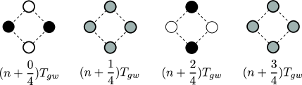
Figure 1: The 4 circles represent 4 pulsars that form a small square on the sky. The timing residuals of all 4 pulsars are oscillating with the same amplitude and period $T_{gw}$, but different phases; each pulsar’s oscillation is $180^{o}$ out of phase with its 2 nearest neighbors. (This figure depicts this by showing 4 different moments in the oscillation cycle: black, white, or grey circles indicate that, at that moment, the pulses are arriving early, late, or “on time,” respectively.) This signature indicates that the square contains a GW point source.

Now consider multiple GW sources. We can repeat the previous section’s counting argument, except that we must now include the $N$ unknown pulsar distances when we are counting the parameters needed to specify the pattern of timing residuals; with this modification, we find that a PTA which monitors $F$ different GW frequency bins can completely characterize up to an average of $(2N/7)(1-1/2F)$ “chirping” sources [or $(2N/6)(1-1/2F)$ monochromatic sources] per bin. Note that, although we didn’t know the pulsar distances a priori, they are determined, in principle, by the fit .

If the PTA can disentangle and characterize the individual sources, how well can they be angularly localized? To answer this question, one should ask, for each combination of pulsar and GW source, whether the fit to the timing residuals has determined $r_{\alpha}$ accurately or poorly relative to $\lambda_{gw}/(1+\hat{n}\cdot\hat{r}_{\alpha})$; roughly speaking, if $r_{\alpha}$ has been determined accurately then we expect the pulsar will contribute diffraction limited angular information as described by Eq. (14); and if $r_{\alpha}$ has been determined poorly then we expect the pulsar will contribute “quasi-singularity limited” angular information $\Gamma_{\bar{\mu}\bar{\nu}}^{\alpha}$ for that source, as described by Eqs. (20) and (21). Consider the localization of a GW source when all of the pulsar’s have poorly known distances; as explained above, the quasi-singular pattern of timing residuals implies that the angular localization will be dominated by the pulsars that are close to that source on the celestial sphere; in particular, it is roughly set by the smallest quadrilateral of pulsars that encircles the source on the celestial sphere, down to a limiting angular resolution of roughly $\delta\theta\sim(1/{\rm SNR}_{\alpha})\sqrt{\lambda_{gw}/d_{pulsar}}$ [the more precise statement is given by Eqs. (20) and (21)]. To understand this behavior, consider the example in Fig. 1.

V Discussion

As we have seen, if a PTA is confronted with too many gravitational wave GW sources, it will become “confused” (unable to disentangle the sources). It was previously assumed (e.g. in SVV ), as a rule of thumb, that PTAs would become confused when there was more than one GW source per frequency bin. In this paper, we have derived the confusion limit, and shown that the actual result is different: a PTA containing N pulsars does not become confused until there are 2N/7 sources per frequency bin (or slightly less, if the pulsar distances are not accurately known); until this threshold is crossed, the PTA is sensitivity limited, not confusion limited. In other words, a PTA with many pulsars is much less confused than the naive rule of thumb would suggest. To translate this into concrete terms, see the lower left hand panel of Figure 2 in Ref. SVV . This figure estimates the expected number of GW sources above a certain minimum timing residual threshold. From it, we see that: the expected number of GW sources per frequency bin with timing residuals above 100 ns (a relatively near-term/achievable threshold) is well below 0.1 in every bin; the expected number of GW sources per frequency bin with timing residuals above 10 ns (a rather ambitious threshold) is well below 10 in every bin; and even the expected number of GW sources per frequency bin with residuals above 1 ns (a very ambitious/futuristic threshold) is well below 100 in every bin. Thus, even in the rather ambitious/futuristic case in which the PTA can detect GW sources with timing residuals as small as 10 ns, if the PTA contains $\gtrsim 35$ quiet pulsars, it will be sensitivity limited rather than confusion limited, even in its lowest frequency bins. And even in the very ambitious/futuristic case in which the PTA can detect GW sources with timing residuals as small as 1 ns, if the PTA contains $\gtrsim 350$ quiet pulsars (see e.g. IPTA ), it will be sensitivity limited rather than confusion limited, even in its lowest frequency bins. (Let us put these numbers in some context. At the moment, there are about 20 pulsars with rms timing residuals less than 1 $\mu$s, and a few pulsars with rms timing residuals as small as 100 ns Demorest et al. (2009). In the nearer term, the Parkes Pulsar Timing Array is aiming to monitor an array of 20 pulsars, each with rms residuals better than 100 ns over a 5 year timescale Manchester2008 . And in the future, the Square Kilometer Array project could detect more than 20,000 pulsars, including hundreds of pulsars with rms timing residuals that match or surpass the best few pulsars currently available Kramer ; IPTA ; SesanaVecchio .) Thus, it is a very plausible possibility that future PTAs will be sensitivity limited, rather than confusion limited, even at their lowest frequencies. In this case, the traditional picture of a PTA as a stochastic background detector will be incorrect, and there will be a significant advantage to analyzing the data via matched filtering (as is done in other gravitational wave experiments such as LIGO LIGO ) and thinking of the PTA as a point source telescope, rather than analyzing it as if it were detecting a stochastic background.

In the previous sections, we have attempted to clarify the limits on the capabilities of PTAs and, in particular, how these limits depend on factors such as the SNR distribution of the GW sources, the number and angular distribution of the pulsars relative to the GW sources, the distances to the pulsars and the precisions of those distances. Our results for the angular resolution were obtained by Fisher matrix methods, assuming gaussian, stationary noise. For this reason, we must remember that in general these results must be interpreted as bounds on (rather than estimates of) the angular resolution. For high-SNR sources, these bounds will be saturated, and may be reinterpreted as actual estimates; for moderate-SNR sources they will still provide useful quantitative guidelines; but for low-SNR sources, it is especially important to remember that our formulae represent bounds rather than estimates, since the Fisher bounds will become increasingly “loose” (i.e. non-saturated) in the low SNR regime Lee . (Note that the relevant SNR here is the total SNR of the source in the PTA, which can be high even if the SNR per pulsar is not.)

In addition to the analytical formulae presented and interpreted earlier, it is worth mentioning one other rule of thumb to keep in mind when estimating the angular resolution of a PTA. Generically, since most pulsars tend to be located in the galactic plane, one expects the spatial resolution to be best for GW sources near the galactic pole if pulsar distances are accurately known, and best for GW sources in the galactic plane if pulsar distances are poorly known.

This paper has focused on the angular resolution of a PTA in the regime where the GW sources are not confused; and on the conditions that need to be satisfied in order to be in this regime. In the opposite (fully confused) regime, the gravitational wave signal may be treated as a Gaussian random field; this situation has been extensively studied in the literature. The intermediate regime in between these two limits is also very interesting, but clearly more complicated than either limit, and will be left for future work.

Other interesting problems for future work include: (i) “tightening” the angular resolution limits at low SNR, beyond the limits obtained by Fisher matrix methods Lee ; (ii) extending this work to GW point sources that are near enough that their wavefront curvature is significant DengFinn ; (iii) determining the circumstances in which pulsar distance determination by GW fitting can compete with more traditional methods (i.e. VLBI, cyclic spectroscopy or timing parallax), see CorbinCornish ; (iv) clarifying the statistics of GW sources which are anomalously well characterized because they are fortuitously located relative to one or several pulsars on the sky; (v) quantifying the gain from matched filtering (with quasi-singular filters in particular) compared to traditional stochastic correlation analysis, even when the PTA appears source confused; (vi) understanding the predicted distribution of frequency derivative $\dot{f}$ among the GW sources relevant to PTAs, and the implications of this distribution for PTA GW telescopes.

Acknowledgements. We are grateful to Chris Hirata, Neil Turok, and Michael Kramer for valuable conversations. LB acknowledges support from the CIFAR JFA. UP received NSERC support for this work.

References

- (1) M.V. Sazhin, Soviet Astronomy 22, 36 (1978).
- (2) S. Detweiler, ApJ 234, 1100 (1979).
- (3) R. Hellings and G. Downs, ApJ 361, 300 (1983).
- Demorest et al. (2009) P. Demorest et al., Astro2010: The Astronomy and Astrophysics Decadal Survey, 2010, 64 [arXiv:0902.2968].
- Verbiest et al. (2009) Verbiest, J. P. W., Bailes, M., Coles, W. A., et al. 2009, MNRAS, 400, 951.
- (6) G. Hobbs et al., Class. Quant. Grav. 27, 084013 (2010).
- (7) F. Jenet et al., arXiv:0909.1058.
- (8) D. R. B. Yardley et al., MNRAS 407, 669 (2010).
- (9) D. R. B. Yardley et al., MNRAS 414, 1777 (2011).
- (10) R. van Haasteren et al., MNRAS 414, 3117 (2011).
- (11) R.S. Foster and D.C. Backer, ApJ 361, 300 (1990).
- (12) F. A. Jenet et al., ApJ 653, 1571 (2006).
- (13) R. van Haasteren et al., MNRAS 395, 1005 (2009).
- (14) P. Demorest et al., arXiv:1201.6641.
- (15) F. A. Jenet et al., ApJ 606, 799 (2004).
- (16) A. Sesana et al., MNRAS 394, 2255 (2009).
- (17) Sesana, A., & Vecchio, A. 2010, Classical and Quantum Gravity, 27, 084016
- (18) L. Finn and A. Lommen, ApJ 718, 1400 (2010).
- (19) A. N. Lommen, arXiv:1112.2158 (2011).
- (20) X. Deng and L.S. Finn, arXiv:1008:0320.
- (21) V. Corbin and N. Cornish, arXiv:1008.1782
- (22) K. J. Lee et al., arXiv:1103.0115.
- (23) C. Misner, K. Thorne and J. Wheeler, Gravitation.
- (24) L. A. Wainstein and V. D. Zubakov, Extraction of Signals from Noise (Dover Publications, Inc., New York, 1962).
- (25) L. S. Finn, Phys. Rev. D 46, 5236 (1992).
- (26) C. Cutler and E. E. Flanagan, Phys. Rev. D 49, 2658 (1994).
- (27) A. T. Deller et al., Astrophy. J. 685, L67 (2008).
- (28) W. F. Brisken, J. M. Benson, W. M. Goss and S. E. Thorsett, Astrophys. J. 571, 906 (2002).
- (29) S. Chatterjee et al., Astrophys. J. 604, 339 (2004).
- (30) S. Chatterjee et al., Astrophys. J. 698, 250 (2009).
- (31) R. Smits et al., Astron. & Astrophys. 528, A108 (2011) [arXiv:1101.5971].
- Demorest (2011) Demorest, P. B. 2011, MNRAS, 416, 2821.
- (33) W.F. Brisken et al., Astrophys. J. 708, 232 (2010).
- Walker et al. (2008) Walker, M. A., Koopmans, L. V. E., Stinebring, D. R., & van Straten, W. 2008, MNRAS, 388, 1214.
- (35) U.-L. Pen and L. King 2012, MNRAS, 421, 132.
- (36) U.-L. Pen et al., in preparation.
- (37) R. N. Manchester, AIP Conf. Proc. 983, 584 (2008) [arXiv:0710.5026].
- (38) M. Kramer et al., New Astron. Rev. 48, 993 (2004) [astro-ph/0409379].
- (39) www.ligo.org