On detecting determinism and nonlinearity in microelectrode recording signals: Approach based on non-stationary surrogate data methods

Abstract

Two new surrogate methods, the Small Shuffle Surrogate (SSS) and the Truncated Fourier Transform Surrogate (TFTS), have been proposed to study whether there are some kind of dynamics in irregular fluctuations and if so whether these dynamics are linear or not, even if this fluctuations are modulated by long term trends. This situation is theoretically incompatible with the assumption underlying previously proposed surrogate methods. We apply the SSS and TFTS methods to microelectrode recording (MER) signals from different brain areas, in order to acquire a deeper understanding of them. Through our methodology we conclude that the irregular fluctuations in MER signals possess some determinism.

I INTRODUCTION

Stereotactic deep brain stimulation is a widespread treatment for different kinds of neurological diseases, especially motor disorders, such as Parkinson’s disease [1]. In this procedure, electrodes are permanently implanted in the patient’s subthalamic nucleus (STNs). They emit signals that reduce the effect of chronic hyperactivity of STN. This treatment is specially suited for long term patients who suffer from side effects of the medical treatment.
One crucial and difficult task for neurosurgeons is locating the target brain area to place a neuro-stimulator. Due to differences between the image based target and the position eventually reached, the neurosurgeon defines the final position of the microelectrode based on the sound and waveform of the microelectrode recording (MER) signal [2]. Since MER signals are time-dependent [3], the detection of each area becomes a very complex task and its accuracy depends on the surgeon’s ability [1].
Recently, there has been a widespread interest in finding an automatic way to identify a brain area based on MER signals. Many approaches have been proposed (e.g., time domain analysis [4], wavelet transform [5], Hilber-Huang transform [1, 6], nonlinear dynamics analysis [7]), but none of these techniques are yet considered as a solution to the problem of automatic classification [7].
What are the characteristics of the underlying system that generate MER signals? (i.e., it is deterministic or stochastic, linear or nonlinear). The answer to this crucial unresolved question could lead to the selection of the best technique for classification. The stationary surrogate data method [8] has been used to answer this question in biomedical signals [9, 10]. The basic approach is to select a pseudo stationary sub-segment of the data, but in MER signals this is still an issue [2].
The methodology we present here is based on novel non-stationary surrogate data methods, with which we attempt to show that MER signals are realizations of a deterministic non-stationary process, contrary to what has been suggested [1, 6].

II Materials and Methods

In this section we present our data base, briefly introduce the basic ideas of the standard surrogate data method and describe the SSS and TFTS methods.

II-A Database

The MER signals used in this study are from the Polytechnic University of Valencia (UPV) and the Technological University of Pereira (UTP). The UPV database acquisition parameters were: Sampling frequency 24 kHz, resolution 16-bits, and 240.000 samples. The UTP acquisition parameters were: Sampling frequency 24 kHz, resolution 16-bits, and 48.000 samples. Each signal was labeled by a neurophysiologists. There are 92 segmentes of Thalamic Nucleus, 105 of Subthalamic Nucleus, 100 of Zona Incerta and 109 of Substantia Nigra pars Reticulata. The surgeries were performed on five patients in Valencia (Spain) using the acquisition equipment LEADPOINT-TM of Medtronic and on five patients in Pereira (Colombia) using the acquisition equipment ISIS-MER of Inomed.

II-B Surrogate data methods

The surrogate data methods test an observed time series against a hierarchy of null hypotheses. The procedure can be described as follows. One starts with an observed time series which is to be tested against the null hypothesis of the surrogate data test. The standard surrogate data repertoire provides algorithms to test against the hypotheses of (i) independent and identically distributed noise; (ii) linearly filtered noise; or (iii) a monotonic nonlinear transformation of linearly filtered noise. Algorithms for each of these three hypotheses generate an ensemble of artificial time series data: the surrogate data. These surrogate data sets are guaranteed to have both the properties associated with the underlying null hypothesis and are also similar to the original observed data. Now, one simply evokes whatever statistic is of interest and compares the value of this statistic computed from the data to the distribution of values elicited from the surrogates. If the statistic value of the data deviates from that of the surrogates, then the null hypothesis may be rejected. Otherwise, it may not.
The three standard surrogate algorithms are known in the literature as (i) Random shuffle surrogates (RS); (ii) Random phase surrogates (RP); and, (iii) Amplitude adjusted Fourier transform (AAFT) surrogates. These techniques are linear surrogate methods. Unfortunately, the application of the surrogate data method is limited to stationary time series [8]; in fact when this method is applied to non-stationary time series the results are unreliable [8]. One possible solution is to split the non-stationary signal into segments which could be considered nearly stationary, find the surrogate for each segment and then put the surrogates of each segments together. However, this procedure is not applicable to data with sudden changes like jumps or spikes [8].

II-C Small Shuffle Surrogates

Recently, T. Nakamura and M. Small [11] proposed a new surrogate data method named Small-Shuffle Surrogate (SSS), the null hypothesis addressed by this algorithm is that irregular fluctuations are independently distributed random variables (i.e there is no short term dynamics or determinism). The SSS method is essentially an extension of the RS surrogate algorithm to non-stationary data. The SSS method can be stated as follow. Let the original data be $\{x_{t}\}$, let $\{i_{t}\}$ be the index of $\{x_{t}\}$. 1) Obtain $\{i^{\ {}^{\prime}}_{t}\}=\{i_{t}\}+\mathcal{N}(0,A^{2})$, 2) let $\{r_{t}\}$ be the index of the sorted $\{i^{\ {}^{\prime}}_{t}\}$ and 3) obtain the surrogate data $\{s_{t}\}$ from $s_{t}=x(r_{t})$.
In this way local structures or correlations in irregular fluctuations are destroyed and global behaviors are preserved.
After applying the method to an extensive number of real and simulated signals T. Nakamura and M. Small [11] found that selecting $A=1$ is a fairly good choice.

II-D Truncated Fourier Transform Surrogates

If the null hypothesis addressed by the SSS algorithm can be rejected, the next question is whether these dynamics are linear or nonlinear. In order to answer this question in non stationary data, T. Nakamura, M. Small and Y. Hirata [12] proposed the truncated Fourier transform surrogate (TFTS) method. The null hypothesis addressed by this algorithm is that irregular fluctuations are generated by a non stationary linear noisy system. The TFTS algorithm works by preserving the low frequency phases in the Fourier transform, but randomizing the high frequency components. The method presented here is an extension of the RS algorithm. 1) Compute the complex Fourier Transform $\{X_{\omega}\}_{\omega}$ of the original data $\{x_{t}\}$, 2) generate random phases $\{\phi_{\omega}\}$ such that $\{\phi_{\omega}\}\sim U(-\pi,\pi)$ if $\omega>f_{c}$, and $\{\phi_{\omega}\}=0$ if $\omega\leq f_{c}$ and 3) obtain the surrogate by computing the inverse Fourier transform of the complex series $\{X_{\omega}e^{\imath\phi_{\omega}}\}_{\omega}$.
While all phases are not randomized in this method it is possible to discriminate between linearity and non-linearity because the superposition principle is valid only for linear data. i.e., when data are nonlinear, even if the power spectrum is preserved completely, the inverse Fourier transform data using randomized phases will exhibit a different dynamical behavior.
The surrogate data generated by this method are influenced primarily by the choice of the cutoff frequency $f_{c}$. If $f_{c}$ is too high, the TFTS data are almost identical to the original data. In this case, even if there is nonlinearity in irregular fluctuations, one may fail to detect nonlinearity. Conversely, if $f_{c}$ is too low, the TFTS data are almost the same as the linear surrogate data and the long-term trends are not preserved. In this case, even if there is no nonlinearity in irregular fluctuations, one may wrongly judge otherwise. The method for selecting the correct value of $f_{c}$ is presented in [12].

III Detecting determinism and nonlinearity

For the detection of determinism and nonlinearity in MER signals we apply the SSS and TFTS methods respectively. The procedure summarized in Fig. 1.

Figure 1: General procedure of the proposed method in order to detect determinism in MER signals.

III-A Preprocessing

Prior to MER signal analysis, raw data is magnified by a preamplifier located near the electrode to reduce electrical noise. After these preconditioning steps, the signal is sampled with an analog-to-digital converter with a sampling rate of 24 kHz. Then an artefact detector is used to eliminate wrong entries in the MER signal due to patient movement. Each MER signal is segmented with a window of 1s, which is considered enough time for identification of brain zones [6].

III-B Selection of the discriminant statistics

Dynamical measures are often used as discriminating statistics. According to [8], the correlation dimension is one of the most popular choices. To estimate these, we first need to reconstruct the underlying attractor. For this purpose, a time-delay embedding reconstruction is usually applied [8]. But this method is not useful for data exhibiting irregular fluctuations and long-term trends. This is because a smaller time delay is necessary to treat irregular fluctuations and a larger time delay is necessary to treat long-term trends. At the moment, there is not a good method for embedding such data [8].
Therefore, as discriminant statistics we chose the Average Mutual Information (AMI) and the Lempel-Ziv Complexity (LZ Complexity) (see [8] for further information). These are selected for four reason: i) Using these statistics we avoid the difficulties associated with embedding; ii) both are widely used in the literature as discriminating statistics [12, 13], iii) it has been shown that LZ complexity is suited to physiological signals [13] and iv) in a separate study we conclude that the obtained result using the correlation dimension as test statistic are the same as when using AMI and LZ Complexity.

III-C Determination of the shortest segment to analyze

In order to determine the shortest segment to analyze, we generated 24 sub-segments from the 1s segment, the first sub-segment of 1000 data points (0.416s) and the last one of 24000 data points (1s), increasing 1000 data points each sub-segment. Then we computed the AMI and LZ complexity for the 24 sub-segments.

III-D Determination of the correct value of $f_{c}$

In order to estimate the correct value of $f_{c}$ we start with a high $f_{c}$ (i.e., we randomize the phases of the highest $5\%$ of the frequency range; in this case the frequency range is $1-12.000$ Hz due to the symmetry of the Fourier coefficients), then if the auto correlation (AC) of the original data falls within the distribution of the surrogates generated with the TFTS algorithm (when the AC of the original data falls within the distribution, linearity and long term trends are sufficiently preserved in the surrogate data, we inspect the AC at time lag 1 because it must be more sensitive to the nature of the data [12]), we decreases the value of $f_{c}$ by a constant rate (i.e., now we randomize the phases of the highest $10\%$ of the frequency range). We keep doing this until we find a value of $f_{c}$ for which the AC of the original data falls outside the distribution of the surrogates, and then the correct value of $f_{c}$ is the last one for which the AC of the original data fell within the distribution of the surrogates.

III-E Application of the SSS and TFTS methods

In order to detect determinism and nonlinearity we generate 39 surrogates for each signal with each method, in this way for a two sided test we achieve $95\%$ confidence, i.e., there is a $5\%$ probability that the null hypothesis is rejected even though it is true.
Then we calculate the AMI at time lag 1 and the LZ complexity for each signal and its surrogates, and check whether the statistics for the original data falls within the distribution of the surrogates. This information lead us to reject or not the null hypothesis.

IV Results and discussion

Following the procedure proposed in III-C, we found that the LZ-complexity and the AMI are well behaved for MER signals with $n>2\times 10^{4}$ (number of data points), so we decided to perform all further analysis with the 1s window. Following III-D we found that by randomizing the phases of the highest $80\%$ of the frequency range, the AC of the data fell outside the distribution of the surrogates, so we decided to randomize the phases only of the higher $75\%$ of the frequency range, in this case with a data length of $24000$ data points we obtained $f_{c}=3000$ Hz.

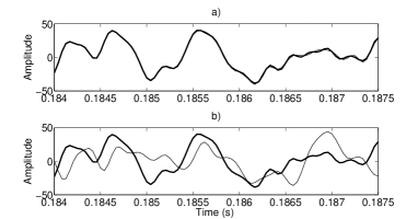
Figure 2: a) Original MER signal and one of the TFTS surrogates (thinner line) with $f_{c}=9600$ Hz b) Original MER signal and one of the TFTS surrogates (thinner line) with $f_{c}=1600$ Hz.

Fig. 2 a) shows the case of too little randomization, while Fig. 2 b) shows the case of too much randomization. In both cases one could wrongly accept or reject a null hypothesis.

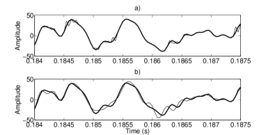
Figure 3: a) Original MER signal and one of the SSS surrogates (thinner line) b) Original MER signal and one of the TFTS surrogates with $f_{c}=7600$ (thinner line)

Fig. 3 shows how both algorithms work, the SSS method randomly destroys the local structures of the data but preserves the long-term behavior, thus one obtains a realization of a non stationary stochastic process; while the TFTS method randomly alters the high frequency components of the signals, whilst preserving the low frequency components, the surrogates preserve the long-term behavior of the data, thus obtaining a realization of a non stationary linear noisy process.
Following the procedure stated in III-E, we found that the hypothesis addressed by the SSS algorithm could be rejected, i.e., we found a statistical difference between the data and the surrogates generated with the SSS algorithm. This implies that the MER signals possess dynamics. Fig. 4 shows the statical difference between the data and the surrogates.

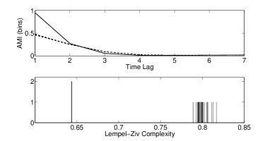
Figure 4: AMI and LZ Complexity for one of the signal (continuous line in the top and the longer stem in the bottom) and the surrogates generated with the SSS algorithm

Applying the TFTS method we encountered that almost $27\%$ of the database rejects the null hypothesis, while the rest of the database was not able no reject it. First, it is necessary to clarify that the fact that we were not able to reject the null hypothesis does not make it true, it just means that the statistical methods found no difference between the original data and the surrogates.
What is unusual here is that not all the database behaves in the same way (regarding the null hypothesis) so, we need to seek an explanation for this phenomenon. If this odd behaviour where caused by a miss application of the TFTS method, the null hypothesis would be rejected or accepted by all the signals of the database (in Fig. 4 we present the result of a miss application of the method). An other possible explanation is that, the 1s window turns out to be stationary. This is possible but very improbable. To prove this, we applied a stationarity test proposed in [14] to the signals that reject the null, we found that all the signals were non stationary.
Finally, we apply the following procedure: We take the 10s signal (for this we only used the UPV database) and divided it into 8 sub-segment of 1s (we did not use the first and last second of the signal), then applied the procedure described in III-E to each sub-segment. We found that each signal poses sub-segments that reject the null and other sub-segments that accept the null. That is, for some time intervals the signal behaves like the realization of a non-stationary linear noisy process and for some other it does not. Fig. 5 shows this result for one of the signals using the LZ complexity as test statistic.

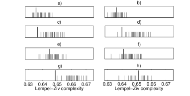
Figure 5: Acceptance (a,b,d,e,f,h) or rejection (c,g) of the null hypothesis addressed by the TFTS method using the LZ complexity.

V Conclusions

Through our methodology we proved that the MER signals are deterministic, this in contrast to what has been guessed by some authors [1, 6]. This implies that there is a dynamic rule that governs the temporal evolution of the signal. Unfortunately due to non-stationarity of the signal, there is not a good method for estimating the dimension of the dynamical system.
We found that there are moments in which the MER signal can be modelled as a realization of a non stationary linear noisy system and others in which it may not, so we might conclude that methodologies such as the wavelet transform or the Hilbert-Huang transform are suited for the analysis of MER signals. We also encourage researchers not to characterize MER signals through methodologies developed for time series that behave like i.i.d. random variables or that are limited to be applied to stationary processes (e.g. Fourier analysis, non linear dynamics analysis).

VI Acknowledgments

We express our sincere appreciation to the Research Center of the Instituto Tecnológico Metropolitano of Medellín - Colombia within the framework of the P09225 grant, Universidad Tecnológica de Pereira and the Créditos Condonables program financed by COLCIENCIAS. We wish to thank T. Nakamura, for his contributions during this study. We also appreciate the comments by two anonymous reviewers.

References

- [1] H. Xue and Z. Qian, “Hibert-huang transform analysis for neuron signal of microelectrode-guided stereotactic neurosurgery for parkinson’s disease,” in ICBBF 2007, Washington, DC, USA, 2007, pp. 1273 – 1276.
- [2] M. Aboy and J. H. Falkenberg, “An automatic algorithm for stationary segmentation of extracellular microelectrode recordings,” Med Biol Eng Comput, vol. 44, p. 511 – 515, 2006.
- [3] Z. Israel and K. J. Burchiel, Microelectrode Recording in Movement Disorder Surgery. Thieme, 2004.
- [4] J. H. Falkenberg, J. McNames, J. Favre, and K. J. Burchiel, “Automatic analysis and data visualization of microelectrode recording trajectories to the subthalamic nucleus: Preliminary results,” Stereotactic and Functional Neurosurgery, vol. 84, no. 1, pp. 35 – 45, 2006.
- [5] P. Gemmar, O. Gronz, T. Henrichs, F. Hertel, and C. Decker, “Mer classification for deep brain stimulation,” in Sixth Heidelberg Innovation Forum, 2008.
- [6] R. Pinzon Morales, M. Garces Arboleda, and A. Orozco Gutierrez, “Automatic identification of various nuclei in the basal ganglia for parkinson’s disease neurosurgery,” in EMBS 2009, Minneapolis, MN, USA, 2009, pp. 3473 – 3476.
- [7] A. Rodríguez, E. Delgado, A. Orozco, G. Castellanos, and E. Guijarro, “Nonlinear dynamics techniques for the detection of the brain areas using mer signals,” in BMEI 2008, Washington, DC, USA, 2008, pp. 198–202.
- [8] M. Small, Applied Nonlinear Time Series Analysis - Applications in Physics, Physiology and Finance. World Scientific, 2005.
- [9] E. Delgado Trejos, G. Castellanos, and M. Vallverdú, Analysis of relevance in representation space oriented to diagnostic support (translate from Spanish). Manizales, Caldas: Universidad Nacional de Colombia, 2009.
- [10] M. Small, D. Yu, J. Simonotto, R. G. Harrison, N. Grubb, and K. Fox, “Uncovering non-linear structure in human ecg recordings,” Chaos, Solitons and Fractals, vol. 13, p. 1755 – 1762, 2002.
- [11] T. Nakamura and M. Small, “Small-shuffle surrogate data: Testing for dynamics in fluctuating data with trends,” Physical Review E, vol. 72, p. 056216, 2005.
- [12] T. Nakamura, M. Small, and Y. Hirata, “Testing for nonlinearity in irregular fluctuations with long-term trends,” Physical Review E, vol. 74, p. 026205, 2006.
- [13] M. Aboy, R. Hornero, D. Abasolo, and D. Alvarez, “Interpretation of the lempel-ziv complexity measure in the context of biomedical signal analysis,” IEEE Trans. on Bio. Eng., vol. 53, no. 11, pp. 2282 – 2288, 2006.
- [14] P. Borgnat and P. Flandrin, “Stationarization via surrogates,” J. Stat. Mech.: Th. and Exp, 2009.