Initial correlations in open system’s dynamics: The Jaynes-Cummings model

Abstract

Employing the trace distance as a measure for the distinguishability of quantum states, we study the influence of initial correlations on the dynamics of open systems. We concentrate on the Jaynes-Cummings model for which the knowledge of the exact joint dynamics of system and reservoir allows the treatment of initial states with arbitrary correlations. As a measure for the correlations in the initial state we consider the trace distance between the system-environment state and the product of its marginal states. In particular, we examine the correlations contained in the thermal equilibrium state for the total system, analyze their dependence on the temperature and on the coupling strength, and demonstrate their connection to the entanglement properties of the eigenstates of the Hamiltonian. A detailed study of the time dependence of the distinguishability of the open system states evolving from the thermal equilibrium state and its corresponding uncorrelated product state shows that the open system dynamically uncovers typical features of the initial correlations.

I Introduction

Quantum systems are typically subjected to the interaction with an environment which influences their dynamics in a non negligible way. A realistic description, taking this external influence into account, is crucial for the theoretical description of open quantum systems, which play an important role in many areas of physics Breuer2007 . The available theoretical tools allow a full characterization for a Markovian dynamics, which can be described by means of completely positive quantum dynamical semigroups Gorini1976a ; Lindblad1976a . However, the assumptions justifying the Markovian description of the open system dynamics are often too restrictive, and a more general analysis is required. A wealth of different approaches to deal with non-Markovian dynamics have been introduced Daffer2004a ; Budini2004a ; Shabani2005a ; Maniscalco2006a ; Vacchini2008a ; Ferraro2008a ; Kossakowski2008a ; Kossakowski2009a ; Breuer2008a ; Breuer2009a ; Piilo2008a ; Piilo2009a ; Breuer2009d ; Breuer2009c ; Laine2010a ; Vacchini2010b ; Smirne2010a ; Chruscinski2010a ; Chruscinski2010b ; Mazzola2010a , but they typically rely on the hypothesis that at the initial time the open system and the environment are statistically independent. This assumption is well justified in the case of weak interaction, but in general one cannot neglect the initial correlations between the open system and the environment Uchiyama2010a ; Pechukas1994a ; Alicki1995a .

Considering an open system $S$ which is coupled to an environment $E$ and assuming that the composite system evolves according to a unitary time evolution operator $U(t)$ from a total initial state $\rho_{SE}(0)$, we can write the state of $S$ at time $t$ as follows,

$$\rho_{S}(t)=\operatorname{Tr}_{E}\left[U(t)\rho_{SE}(0)U^{\dagger}(t)\right].$$ (1)

This equation defines a linear, completely positive and trace preserving map $\Lambda_{t}$ from the state space of the total system $S+E$ to the state space of the open system $S$:

$$\rho_{SE}(0)\mapsto\rho_{S}(t)=\Lambda_{t}\rho_{SE}(0).$$ (2)

If the open system $S$ and its environment $E$ are initially in an uncorrelated tensor product state

$$\rho_{SE}(0)=\rho_{S}(0)\otimes\rho_{E}$$ (3)

with a fixed environmental state $\rho_{E}$, Eq. (1) also defines a linear map $\Phi_{t}$ from the state space of $S$ into itself,

$$\rho_{S}(0)\mapsto\rho_{S}(t)=\Phi_{t}\rho_{S}(0)=\operatorname{Tr}_{E}\left[U(t)\rho_{S}(0)\otimes\rho_{E}U^{\dagger}(t)\right].$$ (4)

It can be shown that this quantum dynamical map $\Phi_{t}$ is again completely positive and trace preserving. Under the additional assumption that the family of dynamical maps $\{\Phi_{t},t\geq 0\}$ constitutes a semigroup, one derives the general mathematical structure of its generator, which leads to the widely-used quantum Markovian master equations for the open system state $\rho_{S}(t)$ in Lindblad form.

The above construction of the quantum dynamical map $\Phi_{t}$ presupposes that one restricts the class of initial conditions to states of the form of Eq. (3), where $\rho_{E}$ is a fixed, given environmental state. Thus, a large class of initial conditions is excluded when considering dynamical maps acting on the reduced state space, in particular those initial conditions that describe correlations and entanglement between system and environment. On the other hand, it is a well known fact that correlations in the initial state can have strong influences on the open system dynamics, both in thermal equilibrium and in non-equilibrium systems. The question is thus, how do initial correlations affect the reduced system dynamics, and what are appropriate observable measures that quantify such effects? Here, we discuss these questions in detail with the help of the example of the Jaynes-Cummings model, the model of a two-state system coupled to a bosonic field mode, employing the analytical representation of the reduced dynamics of this model for arbitrary initial states Smirne2010b .

It should be mentioned that under certain additional assumptions Eq. (1) can indeed be used to construct maps on the reduced state space to represent the dynamics in the case of initial correlations vanWonderen2000a ; Stelmachovic2001a ; Jordan2004a ; Rodriguez2008a ; Carteret2008a ; Shabani2009a . However, this construction demands that the initial correlations between the system and its environment are fixed. It turns out that the dynamical maps arising in this way may be not completely positive, and not even positive. This requires the determination of a certain compatibility domain in the physical state space, which is a very complicated mathematical task. In the present paper we shall follow an entirely different strategy, to analyze the role of initial correlations. Namely, in order to quantify the effect of initial system-environment correlations in the subsequent time evolution of the open system, we will investigate the trace distance $D(\rho_{S}^{1}(t),\rho_{S}^{2}(t))$ between a pair of states $\rho^{1}_{S}(t)$ and $\rho^{2}_{S}(t)$ of $S$, which evolve from a given pair of initial states $\rho^{1}_{SE}(0)$ and $\rho^{2}_{SE}(0)$ of the total system. This approach has also been used in Breuer2009c ; Laine2010a to construct a measure for the non-Markovianity of quantum processes, and in Laine2010b to develop a witness which allows the detection of initial correlations through only local measurements on the open system. An application to a specific system has been recently considered in Dajka2010a .

In the present paper we will address, in particular, the situation in which $\rho_{SE}^{1}(0)$ represents a thermal equilibrium (Gibbs) state corresponding to the full Hamiltonian of the model. Since this correlated state is invariant under the time evolution, its reduced states $\rho_{S}^{1}(0)={\rm{Tr}}_{E}\rho_{SE}^{1}(0)$ and $\rho_{E}^{1}(0)={\rm{Tr}}_{S}\rho_{SE}^{1}(0)$ remain of course time independent. However, the initial state $\rho_{SE}^{2}(0)=\rho_{S}^{1}(0)\otimes\rho_{E}^{1}(0)$ given by the product of the marginals does evolve in time, and we will investigate the dynamics of the trace distance $D(\rho_{S}^{1}(t),\rho_{S}^{2}(t))$ between the open system states corresponding to the initial states $\rho_{SE}^{1}(0)$ and $\rho_{SE}^{2}(0)$. For this case the trace distance is bounded from above by the trace distance $D(\rho^{1}_{SE}(0),\rho^{1}_{S}(0)\otimes\rho^{1}_{E}(0))$ which provides a measure for the amount of correlations in the initial Gibbs state Laine2010b . Analyzing in detail the dependence on the temperature and on the system-environment coupling strength, we demonstrate that at small temperatures characteristic properties of these correlations are related to the eigenvalue spectrum and, in particular, to the quantum correlations and the entanglement structure of the eigenstates of $H$. We will discuss further the signatures of these properties in the subsequent dynamics of the open system states. It will be shown that, in fact, the open system dynamically uncovers typical features of the correlations in the initial states.

The paper is organized as follows. In Sec. II we introduce the trace distance and show its relevance as a measure of the distinguishability of two quantum states and of the correlations contained in a given bipartite state. We further consider the exact reduced dynamics of the Jaynes-Cummings model, and study as an example the time behavior of the distinguishability of distinct initial states. In Sec. III we provide a detailed study of the correlations contained in the Gibbs state associated to the Jaynes-Cummings Hamiltonian, as measured by the trace distance between the state and the tensor product of its marginals. We then investigate the time dependence of the distinguishability of the corresponding time evolved states.

II Trace distance and initial system-environment correlations

II.1 General theory

II.1.1 Properties and physical interpretation of the trace distance

The trace distance of two trace class operators $A$ and $B$ is defined as $\frac{1}{2}$ times the trace norm of $A-B$,

$$D(A,B)=\frac{1}{2}||A-B||_{1},$$ (5)

where the trace norm of an operator $X$ is defined by

$$||X||_{1}={\rm{Tr}}|X|={\rm{Tr}}\sqrt{X^{\dagger}X}.$$ (6)

If $X$ is trace class and self-adjoint with eigenvalues $x_{i}$, this formula reduces to the sum of the absolute eigenvalues (counting multiplicity),

$$||X||_{1}=\sum_{i}|x_{i}|.$$ (7)

The trace distance of two quantum states, represented by positive operators $\rho^{1}$ and $\rho^{2}$ with unit trace, is thus given by

$$D(\rho^{1},\rho^{2})=\frac{1}{2}||\rho^{1}-\rho^{2}||_{1}=\frac{1}{2}\operatorname{Tr}|\rho^{1}-\rho^{2}|.$$ (8)

The trace distance is a metric on the space of physical states with several nice properties which make it a useful measure for the distance between two quantum states. We list some of them:

1.

The trace distance for any pair of states satisfies the inequality

$$0\leq D(\rho^{1},\rho^{2})\leq 1,$$ (9)

where $D(\rho^{1},\rho^{2})=0$ if and only if $\rho^{1}=\rho^{2}$, and $D(\rho^{1},\rho^{2})=1$ if and only if $\rho^{1}$ and $\rho^{2}$ have orthogonal supports.

2.

Being a metric, the trace distance satisfies the triangular inequality,

$$D(\rho^{1},\rho^{2})\leq D(\rho^{1},\rho^{3})+D(\rho^{3},\rho^{2}).$$ (10)

3.

All trace preserving positive maps $\Lambda$ are contractions of the trace distance Ruskai1994a ,

$$D(\Lambda\rho^{1},\Lambda\rho^{2})\leq D(\rho^{1},\rho^{2}),$$ (11)

where the equality sign holds if $\Lambda$ is a unitary transformation.

4.

The trace distance is subadditive with respect to the tensor product,

$$D(\rho^{1}\otimes\sigma^{1},\rho^{2}\otimes\sigma^{2})\leq D(\rho^{1},\rho^{2})+D(\sigma^{1},\sigma^{2}).$$ (12)

In particular, one has

$$D(\rho^{1}\otimes\sigma,\rho^{2}\otimes\sigma)=D(\rho^{1},\rho^{2}).$$ (13)

5.

The trace distance can be represented as a maximum taken over all projection operators $\Pi$,

$$D(\rho^{1},\rho^{2})=\max_{\Pi}{\rm{Tr}}\left\{\Pi\left(\rho^{1}-\rho^{2}\right)\right\}.$$ (14)

The physical interpretation Gilchrist2005a of the trace distance is based on the relation (14). Suppose Alice prepares a system in one of two quantum state $\rho^{1}$ and $\rho^{2}$ with probability of $1/2$ each. She gives the system to Bob, who performs a measurement in order to distinguish the two states. Employing Eq. (14) one can show that the maximal success probability for Bob to identify correctly the state is given by $\left[1+D(\rho^{1},\rho^{2})\right]/2$. This means that the trace distance represents the maximal bias in favor of the correct state identification which Bob can achieve through an optimal strategy. Hence, the trace distance $D(\rho_{1},\rho_{2})$ can be interpreted as a measure for the distinguishability of the states $\rho^{1}$ and $\rho^{2}$.

II.1.2 Dynamics of the trace distance

We consider any two total system initial states $\rho^{1}_{SE}(0)$ and $\rho^{2}_{SE}(0)$, and the corresponding open system states $\rho^{1}_{S}(t)$ and $\rho^{2}_{S}(t)$ at time $t$. According to Eqs. (1) and (2) the latter are given by $\rho^{1}_{S}(t)=\Lambda_{t}\rho_{SE}^{1}(0)$ and $\rho^{2}_{S}(t)=\Lambda_{t}\rho_{SE}^{2}(0)$. Since $\Lambda_{t}$ is completely positive and trace preserving, we obtain from Eq. (11) a bound for the trace distance between the reduced system states,

$$D(\rho^{1}_{S}(t),\rho^{2}_{S}(t))\leq D(\rho^{1}_{SE}(0),\rho^{2}_{SE}(0)).$$ (15)

If the initial states are uncorrelated with the same environmental state $\rho_{E}$, that is $\rho^{1}_{SE}(0)=\rho_{S}^{1}(0)\otimes\rho_{E}(0)$ and $\rho^{2}_{SE}(0)=\rho_{S}^{2}(0)\otimes\rho_{E}(0)$, this inequality reduces with the help of (13) to the contraction property for the dynamical map (4),

$$D(\rho^{1}_{S}(t),\rho^{2}_{S}(t))\leq D(\rho^{1}_{S}(0),\rho^{2}_{S}(0)).$$ (16)

This means that for initially uncorrelated total system states and identical environmental states the trace distance between the reduced system states at time $t$ can never be larger than its initial value.

The inequality (15) may be written as

$$D(\rho^{1}_{S}(t),\rho^{2}_{S}(t))-D(\rho^{1}_{S}(0),\rho^{2}_{S}(0))$$

$$\leq D(\rho^{1}_{SE}(0),\rho^{2}_{SE}(0))-D(\rho^{1}_{S}(0),\rho^{2}_{S}(0))$$

$$\equiv I(\rho^{1}_{SE}(0),\rho^{2}_{SE}(0)).$$ (17)

According to this inequality the change of the trace distance of the open system states is bounded from above by the quantity $I(\rho^{1}_{SE}(0),\rho^{2}_{SE}(0))\geq 0$. This quantity represents the distinguishability of the total system initial states minus the distinguishability of the corresponding reduced system initial states. Thus, $I(\rho^{1}_{SE},\rho^{2}_{SE})$ can be interpreted as the relative information of the total initial states which is initially outside the open system, i.e., which is inaccessible for local measurement performed on the open system Laine2010b .

For $I(\rho^{1}_{SE}(0),\rho^{2}_{SE}(0))>0$ the trace distance of the open system states can increase over its initial value. This increase can be interpreted by saying that information which is initially outside the open system flows back to the system and becomes accessible through local measurements. Note that, as will be illustrated by means of several examples below, the bound for the dynamics of the trace distance given by Eq. (17) is tight, i.e., it can be reached for certain total initial states. If the bound of inequality (17) is actually reached at some time $t$, the initial distinguishability of the total system states is equal to the distinguishability of the open system states at time $t$. This means that the relative information on the total initial states has been dynamically transferred completely to the open system Laine2010b .

Using the sub-additivity of the trace distance (12) and the triangular inequality (10) one deduces from (17) the following inequality Laine2010b ,

$$D(\rho_{S}^{1}(t),\rho_{S}^{2}(t))-D(\rho_{S}^{1}(0),\rho_{S}^{2}(0))$$

$$\leq D(\rho_{SE}^{1}(0),\rho_{S}^{1}(0)\otimes\rho_{E}^{1}(0))$$

$$+D(\rho_{SE}^{2}(0),\rho_{S}^{2}(0)\otimes\rho_{E}^{2}(0))+D(\rho_{E}^{1}(0),\rho_{E}^{2}(0)).$$ (18)

For any state $\rho_{SE}$ the quantity $D(\rho_{SE},\rho_{S}\otimes\rho_{E})$ describes how well $\rho_{SE}$ can be distinguished from the fully uncorrelated product state $\rho_{S}\otimes\rho_{E}$ of its marginal states $\rho_{S}$ and $\rho_{E}$. Thus, $D(\rho_{SE},\rho_{S}\otimes\rho_{E})$ can be interpreted as a measure for the total amount of correlations in the state $\rho_{SE}$. Therefore, the inequality (II.1.2) shows that an increase of the trace distance of the open system states over its initial value implies that there must be correlations in the initial states $\rho_{SE}^{1}(0)$ or $\rho_{SE}^{2}(0)$, or that the environmental states are different. An important special case, which will be considered in detail in the present paper, occurs if $\rho^{2}_{SE}(0)$ is given by the product state obtained from the marginals of $\rho^{1}_{SE}(0)$, i.e., $\rho^{2}_{SE}(0)=\rho^{1}_{S}(0)\otimes\rho^{1}_{E}(0)$. The inequality (17) then reduces to the simple form

$$D(\rho^{1}_{S}(t),\rho^{2}_{S}(t))\leq D(\rho^{1}_{SE}(0),\rho^{1}_{S}(0)\otimes\rho^{1}_{E}(0)),$$ (19)

according to which the increase of the trace distance is bounded by the amount of correlations in the total initial state Laine2010b .

II.2 Example: The Jaynes-Cummings model

II.2.1 The physical model

We consider a two-state system coupled to a single mode of the radiation field with total Hamiltonian

$$H = H_{S}+H_{E}+H_{I}$$ (20)

$$= \omega_{0}\sigma_{+}\sigma_{-}+\omega b^{{\dagger}}b+g\left(\sigma_{+}\otimes b+\sigma_{-}\otimes b^{{\dagger}}\right),$$

where $\sigma_{+}=|1\rangle\langle 0|$ and $\sigma_{-}=|0\rangle\langle 1|$ are the raising and lowering operators of the two-state system, $b^{{\dagger}}$ and $b$ are the creation and annihilation operators of the field mode, and the coupling term is in the Jaynes-Cummings form. This model describes, e.g., the interaction between a two-level atom and a mode of the radiation field in the electric dipole and rotating wave approximation. In the interaction picture the Hamiltonian takes the form

$$H_{I}(t)=g\left(\sigma_{+}\otimes be^{i\Delta t}+\sigma_{-}\otimes b^{{\dagger}}e^{-i\Delta t}\right),$$ (21)

where $\Delta=\omega_{0}-\omega$ denotes the detuning between the system’s transition frequency $\omega_{0}$ and the frequency $\omega$ of the field mode. The exact time-evolution operator for the total system in the interaction picture can then be written as (see, e.g., Ref. Puri2001 ):

$$U(t)=\left(\begin{array}[]{cc}c(\hat{n}+1,t)&d(\hat{n}+1,t)b\\ -b^{{\dagger}}d^{{\dagger}}(\hat{n}+1,t)&c^{{\dagger}}(\hat{n},t)\end{array}\right),$$ (22)

where we have introduced the following functions of the number operator $\hat{n}=b^{{\dagger}}b$,

$$c(\hat{n},t) = e^{i\Delta t/2}\left[\cos\left(\Omega(\hat{n})\frac{t}{2}\right)-i\frac{\Delta}{\Omega(\hat{n})}\sin\left(\Omega(\hat{n})\frac{t}{2}\right)\right],$$

$$d(\hat{n},t) = -ie^{i\Delta t/2}\frac{2g}{\Omega(\hat{n})}\sin\left(\Omega(\hat{n})\frac{t}{2}\right),$$ (23)

with

$$\Omega(\hat{n})=\sqrt{\Delta^{2}+4g^{2}\hat{n}}.$$ (24)

With the help of the unitary time-evolution operator given by Eq. (22) we can easily determine the exact expression for the reduced density matrix of the two-level system at time $t$,

$$\rho_{S}(t)=\left(\begin{array}[]{cc}\rho_{11}(t)&\rho_{10}(t)\\ \rho^{\ast}_{10}(t)&\rho_{00}(t)\end{array}\right),$$ (25)

corresponding to an arbitrary initial state $\rho_{SE}(0)$ of the total system. First, we expand $\rho_{SE}(0)$ with respect to the basis vectors $|\alpha\rangle\otimes|n\rangle\equiv|\alpha,n\rangle$, where $\alpha=1,0$ labels the states of the two-state system, and $n=0,1,2,\ldots$ the number states of the field mode,

$$\rho_{SE}(0)=\sum_{\alpha,\beta,m,n}\rho^{mn}_{\alpha\beta}(0)|\alpha,m\rangle\langle\beta,n|.$$ (26)

Substituting this expression into Eq. (1) with $U(t)$ given by Eq. (22), one obtains

$$\rho_{11}(t)=\sum_{n}\left[\rho^{nn}_{11}(0)|c_{n+1}(t)|^{2}+2\sqrt{n+1}\right.$$

$$\left.\times\operatorname{Re}\left\{\rho^{n,n+1}_{10}(0)d^{\ast}_{n+1}(t)c_{n+1}(t)\right\}+n\rho^{nn}_{00}(0)|d_{n}(t)|^{2}\right]$$

$$\rho_{10}(t)=\sum_{n}\left[-\sqrt{n+1}\rho^{n+1,n}_{11}(0)c_{n+2}(t)d_{n+1}(t)\right.$$

$$\left.-\sqrt{n+2}\sqrt{n+1}\rho^{n+2,n}_{01}(0)d_{n+2}(t)d_{n+1}(t)\right.$$

$$\left.+\rho^{nn}_{10}(0)c_{n+1}(t)c_{n}(t)+\sqrt{n+1}\rho^{n+1,n}_{00}(0)d_{n+1}(t)c_{n}(t)\right],$$

(27)

where $c_{n}(t)$ and $d_{n}(t)$ denote the eigenvalues of $c(\hat{n},t)$ and $d(\hat{n},t)$ corresponding to the eigenstate $|n\rangle$, respectively.

We note that Eq. (27) does in general not lead to a dynamical map for the state changes of the reduced two-state system since it is not possible to write the right-hand side of this equation as a function of the matrix elements of the reduced initial state $\rho_{S}(0)$ which are given by

$$\rho_{\alpha\beta}(0)=\sum_{n}\rho^{nn}_{\alpha\beta}(0).$$ (28)

However, if the total initial state is of tensor product form, $\rho_{SE}(0)=\rho_{S}(0)\otimes\rho_{E}(0)$ and, therefore,

$$\rho^{nm}_{\alpha\beta}(0)=\rho_{\alpha\beta}(0)\rho^{nm}(0),$$ (29)

it is indeed possible to construct the dynamical map; if moreover $\left[\rho_{E}(0),\hat{n}\right]=0$, one finds the map already derived in Ref. Smirne2010b .

II.2.2 Dynamics of the trace distance for pure or product total initial states

We illustrate the dynamics of the trace distance and the inequality (17) by means of two simple examples, considering the situation in which the total initial state is a product state or a pure state. The case of a mixed, correlated initial state will be considered in detail in Sec. III.

The quantity on the right-hand side of Eq. (17), representing the information which is initially outside the reduced system, can be larger than zero basically for two reasons: First, because one has different environmental initial states $\rho^{1}_{E}(0)$ and $\rho^{2}_{E}(0)$ and, second, because of the presence of correlations in the initial states $\rho^{1}_{SE}(0)$ or $\rho^{2}_{SE}(0)$ (see inequality (II.1.2)). To illustrate the first case we study the trace distance between the two reduced states $\rho^{1}_{S}(t)$ and $\rho^{2}_{S}(t)$ evolving from two product initial states with the same reduced system state, namely from $\rho_{SE}^{1}(0)=\rho_{S}(0)\otimes\rho^{1}_{E}(0)$ and $\rho_{SE}^{2}(0)=\rho_{S}(0)\otimes\rho^{2}_{E}(0)$, where

$$\rho_{S}(0)=|\alpha_{1}|^{2}|0\rangle\langle 0|+|\beta_{1}|^{2}|1\rangle\langle 1|$$ (30)

and the two environmental states are taken to be

$$\rho^{i}_{E}(0)=|\alpha_{i}|^{2}|n\rangle\langle n|+|\beta_{i}|^{2}|n-1\rangle\langle n-1|,\qquad i=1,2,$$ (31)

with the normalization condition $|\alpha_{i}|^{2}+|\beta_{i}|^{2}=1$. Numerical simulation results for this case are shown in Fig. (1.a). We see from the figure that the bound of Eq. (17), which is given by $\left||\alpha_{1}|^{2}-|\alpha_{2}|^{2}\right|$, is indeed reached here. For a study of the second case we consider an initially correlated pure state of the form

$$\rho^{1}_{SE}(0)=|\psi\rangle\langle\psi|,$$ (32)

with $|\psi\rangle=\alpha|0,n\rangle+\beta|1,n-1\rangle$, $|\alpha|^{2}+|\beta|^{2}=1$, together with an initial product state of the form

$$\rho^{2}_{SE}(0)=\rho^{2}_{S}(0)\otimes\rho^{2}_{E}(0)$$ (33)

with $\rho^{2}_{S}(0)=|\beta|^{2}|0\rangle\langle 0|+|\alpha|^{2}|1\rangle\langle 1|$ and $\rho^{2}_{E}(0)=|\alpha|^{2}|n\rangle\langle n|+|\beta|^{2}|n-1\rangle\langle n-1|$. Note that $\rho^{2}_{SE}(0)$ is not equal to the product of the marginals of $\rho^{1}_{SE}(0)$. As can be seen from Fig. (1.b) also for this case the bound of Eq. (17), which is given by $\frac{1}{2}(1+|\alpha|^{4}+|\beta|^{4})$, is repeatedly reached in the course of time. As expected, in both cases the trace distance of the states exceeds its initial value, corresponding to the fact that the reduced system dynamically retrieves the information initially not accessible to it, related to the different initial environmental states or to the initial system-environment correlations. Note that the trace distance starts increasing already at the initial time, indicating that the information is flowing to the reduced system from the very beginning of the dynamics. Moreover, it keeps oscillating also for large values of $t$, so that the distinguishability growth between reduced states can be detected, e.g. by quantum state tomography, also making observations after a long interaction time.

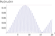
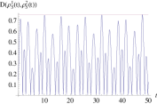
Figure 1: (Color online) Plot of the trace distance $D(\rho^{1}_{S}(t),\rho^{2}_{S}(t))$ as a function of time, where $\rho_{S}^{1}(t)$ and $\rho_{S}^{2}(t)$ have been determined from Eq. (27). In both figures the horizontal line marks the upper bound of Eq. (17), and $\Delta=0.1,g=1$ (arbitrary units). (a) Dynamics for two product total initial states which differ only by the environmental states and are given by Eq. (30) and (31) with $|\alpha_{1}|^{2}=7/9$, $|\alpha_{2}|^{2}=8/9$ and $n=7$. (b) The two reduced states $\rho^{1}_{S}(t)$ and $\rho^{2}_{S}(t)$ are obtained from the total initial states given by Eqs. (32) and (33) which have the same environmental marginal state, but different reduced system states and correlations. Parameters: $\alpha=i\sqrt{3/7}$, $\beta=\sqrt{4/7}$ and $n=1$.

In both situations considered and visualized in Fig. (1) the maximum value of the trace distance as a function of time is equal to the upper bound given by Eq. (17), indicating that the information initially inaccessible to the reduced system has been transferred completely to it during the subsequent dynamics. This is of course not always the case and it is an important problem to characterize explicitly those initial states for which such a behavior indeed occurs. Let us consider the special case given by Eq. (19), in which the two total initial states are a correlated state and the tensor product of its marginals, taking $\rho^{1}_{SE}(0)$ to be a pure entangled state, i.e., $\rho^{1}_{SE}(0)=|\psi\rangle\langle\psi|$ with $|\psi\rangle=\alpha|0,n\rangle+\beta|1,m\rangle$. For this case Eq. (27) leads to

$$D(\rho^{1}_{S}(t),\rho^{2}_{S}(t))=\left||\alpha\beta|^{2}(|c_{m+1}(t)|^{2}-|c_{n}(t)|^{2}+|c_{m}(t)|^{2}\right.$$

$$\left.-|c_{n+1}(t)|^{2})+2\delta_{m,n-1}\sqrt{n}\operatorname{Re}\left\{\alpha^{\ast}\beta d^{\ast}_{n}(t)c_{n}(t)\right\}\right|,$$ (34)

while the right-hand side of Eq. (19) becomes

$$D\left(\rho^{1}_{SE}(0),\rho^{1}_{S}(0)\otimes\rho^{1}_{E}(0)\right)=|\alpha\beta|^{2}+|\alpha\beta|.$$ (35)

Taking into account Eq. (23) and Eq. (24), for $n,m\gg\Delta^{2}/4g^{2}$ Eq. (34) explicitly reads

$$D(\rho^{1}_{S}(t),\rho^{2}_{S}(t)) = \Big{|}|\alpha\beta|^{2}\left[\cos^{2}\left(g\sqrt{m+1}t\right)-\cos^{2}\left(g\sqrt{n}t\right)\right.$$ (36)

$$\left.+\cos^{2}\left(g\sqrt{m}t\right)-\cos^{2}\left(g\sqrt{n+1}t\right)\right]$$

$$-\delta_{m,n-1}\operatorname{Im}\left\{\alpha^{\ast}\beta\right\}\sin\left(2g\sqrt{n}t\right)\Big{|},$$

which is an almost periodic function Corduneanu1989 since it represents a linear combination of sine and cosine functions with incommensurable periods. The supremum of the attained values Note1 is less than or equal to $2|\alpha\beta|^{2}$ if $m\neq n$ and $m\neq n-1$, and equal to $|\alpha\beta|^{2}+|\operatorname{Im}\left\{\alpha^{\ast}\beta\right\}|$ if $m=n-1$. Thus, the inequality in Eq. (19) is tight only for those initial states for which $m=n-1$ and $\operatorname{Re}\left\{\alpha^{\ast}\beta\right\}=0$ (indeed, we have $|\alpha\beta|^{2}+|\alpha\beta|=2|\alpha\beta|^{2}$ if and only if either $\alpha=0$ or $\beta=0$). The special role of the initial states with $m=n-1$ can be traced back to the structure of the full unitary evolution given by Eq. (22) and to the presence of the creation and annihilation operators in the off-diagonal matrix elements. Their action generates, in fact, the last term in the modulus on the right-hand side of Eq. (36), which for $m=n-1$ is necessary to reach the bound. If the relation $n,m\gg\Delta^{2}/4g^{2}$ is not satisfied, the supremum lies in general strictly below the bound even if the above mentioned conditions are fulfilled. This is a consequence of the fact that the periodic functions $|c_{n}(t)|^{2}$ are then strictly less than 1.

III Gibbs initial state and dynamics of the trace distance

We now extend our considerations to the evolution of the trace distance between a mixed correlated initial state and the tensor product of its marginals. Specifically, we will analyze the inequality given in Eq. (19) when the correlated initial state $\rho_{SE}$ is the invariant Gibbs (thermal equilibrium) state corresponding to the full Hamiltonian $H$ of the model. For simplicity we will omit in the following the time argument zero. We first analyze the total amount of correlations in the initial state $D\left(\rho_{SE},\rho_{S}\otimes\rho_{E}\right)$, i.e., the upper bound for the trace distance according to Eq. (19). As we shall show below the main features of this bound can be explained in terms of the correlations in the ground state of the Hamiltonian $H$. We further study the behavior of the actual dynamics of the trace distance, which will turn out to reflect the characteristic features of the correlations in the Gibbs state.

III.1 Correlations in the Gibbs state

We consider the total initial Gibbs state

$$\rho_{SE}=\frac{1}{Z}e^{-\beta H},$$ (37)

where $H$ is the total Hamiltonian of the system given by Eq. (20), $Z=\operatorname{Tr}e^{-\beta H}$ denotes the partition function and $\beta=1/k_{b}T$ with $k_{b}$ the Boltzmann constant and $T$ the temperature. To calculate the marginal states $\rho_{S}=\operatorname{Tr}_{E}e^{-\beta H}/Z$ and $\rho_{E}=\operatorname{Tr}_{S}e^{-\beta H}/Z$ it is useful to obtain the matrix elements of $\rho_{SE}$ with respect to the basis $\left\{|\alpha,n\rangle\right\}$ already introduced in Sec. II.2. This can be done using the dressed states Meystre1991a , i.e., the eigenvectors of the Hamiltonian $H$. These eigenvectors can be written as

$$|\Phi^{+}_{n}\rangle = a_{n}|1,n-1\rangle+b_{n}|0,n\rangle,\hskip 20.00003pt$$

$$|\Phi^{-}_{n}\rangle = -b_{n}|1,n-1\rangle+a_{n}|0,n\rangle,\hskip 10.00002pt$$

$$|\Phi^{-}_{0}\rangle = |0,0\rangle,$$ (38)

with $n=1,2,3,\ldots$ and

$$a_{n}=\sqrt{\frac{\Omega_{n}+\Delta}{2\Omega_{n}}},\hskip 20.00003ptb_{n}=\sqrt{\frac{\Omega_{n}-\Delta}{2\Omega_{n}}},$$ (39)

where $\Omega_{n}=\sqrt{\Delta^{2}+4g^{2}n}$ (see Eq. (24)). The corresponding eigenvalues are given by

$$E^{\pm}_{n} = n\omega+\frac{\Delta}{2}\pm\frac{\Omega_{n}}{2},$$

$$E^{-}_{0} = 0.$$ (40)

Inverting Eqs. (38) with the help of the relations

$$|0,n\rangle = b_{n}|\Phi^{+}_{n}\rangle+a_{n}|\Phi^{-}_{n}\rangle,$$

$$|1,n\rangle = a_{n+1}|\Phi^{+}_{n+1}\rangle-b_{n+1}|\Phi^{-}_{n+1}\rangle,$$ (41)

one obtains the expressions

$$\rho^{nm}_{00} = \frac{1}{Z}\delta_{n,m}\left(e^{-\beta E^{+}_{n}}b_{n}^{2}+e^{-\beta E^{-}_{n}}a_{n}^{2}\right),$$

$$\rho^{nm}_{11} = \frac{1}{Z}\delta_{n,m}\left(e^{-\beta E^{+}_{n+1}}a_{n+1}^{2}+e^{-\beta E^{-}_{n+1}}b_{n+1}^{2}\right),$$

$$\rho^{nm}_{10}=\rho^{mn}_{01} = \frac{1}{Z}\delta_{n+1,m}\left(e^{-\beta E^{+}_{n+1}}-e^{-\beta E^{-}_{n+1}}\right)a_{n+1}b_{n+1},$$

which represent the matrix elements of the Gibbs state,

$$\rho_{SE}=\sum_{\alpha,\beta,n,m}\rho^{nm}_{\alpha\beta}|\alpha,n\rangle\langle\beta,m|.$$ (43)

Using this result together with Eq. (28) we see that the reduced system state is diagonal in the basis $|\alpha,n\rangle$ and that the diagonal elements are given by $\rho_{11}=1-\rho_{00}$ and

$$\rho_{00}=\frac{1}{Z}\sum_{n=0}^{\infty}\left(e^{-\beta E^{+}_{n}}b_{n}^{2}+e^{-\beta E^{-}_{n}}a_{n}^{2}\right).$$ (44)

The reduced state of the environment is also diagonal since $\rho^{nm}=0$ for $n\neq m$, and the diagonal elements can be expressed as

$$\rho^{nn} = \frac{1}{Z}\left(e^{-\beta E^{+}_{n}}b_{n}^{2}+e^{-\beta E^{-}_{n}}a_{n}^{2}\right.$$ (45)

$$\left.+e^{-\beta E^{+}_{n+1}}a_{n+1}^{2}+e^{-\beta E^{-}_{n+1}}b_{n+1}^{2}\right).$$

The product state constructed from the marginals is accordingly of the form

$$\rho_{S}\otimes\rho_{E} = \sum_{\alpha,n}\rho_{\alpha\alpha}\rho^{nn}|\alpha,n\rangle\langle\alpha,n|.$$ (46)

Finally, the normalization constant $Z$ can be written as

$$Z = \sum_{n}\left(e^{-\beta E^{+}_{n}}b_{n}^{2}+e^{-\beta E^{-}_{n}}a_{n}^{2}\right.$$ (47)

$$+\left.e^{-\beta E^{+}_{n+1}}a_{n+1}^{2}+e^{-\beta E^{-}_{n+1}}b_{n+1}^{2}\right).$$

Starting from the above relations we can analytically calculate the total amount of correlations of the Gibbs state, i.e., the quantity $D(\rho_{SE},\rho_{S}\otimes\rho_{E})$. To this end, we order the elements of the basis as $\left\{|0,0\rangle,|1,0\rangle,|0,1\rangle,|1,1\rangle,|0,2\rangle,|1,2\rangle,\ldots\right\}$. The difference $X=\rho_{SE}-\rho_{S}\otimes\rho_{E}$ between the Gibbs state and its corresponding product state can then be written in block diagonal form,

$$X=\left(\begin{array}[]{cccccccc}D^{0}_{0}&0&0&0&0&0&\ldots&\ldots\\ 0&D^{0}_{1}&\rho^{01}_{10}&0&0&0&\ldots&\ldots\\ 0&\rho^{10}_{01}&D^{1}_{0}&0&0&0&\ldots&\ldots\\ 0&0&0&D^{1}_{1}&\rho^{12}_{10}&0&\ldots&\ldots\\ 0&0&0&\rho^{21}_{01}&D^{2}_{0}&0&\ldots&\ldots\\ 0&0&0&0&0&\ddots&0&0\\ \vdots&\vdots&\vdots&\vdots&\vdots&D^{n}_{1}&\rho^{n,n+1}_{10}&0\\ \vdots&\vdots&\vdots&\vdots&\vdots&\rho^{n+1,n}_{01}&D^{n+1}_{0}&0\\ \vdots&\vdots&\vdots&\vdots&\vdots&0&0&\ddots\end{array}\right),$$ (48)

where

$$D^{n}_{\alpha} = \rho^{n,n}_{\alpha,\alpha}-\rho_{\alpha,\alpha}\rho^{n,n}.$$ (49)

It is easy to demonstrate that $D^{n}_{1}=-D^{n}_{0}$, implying that the matrix of Eq. (48) has zero trace, as it should be. The eigenvalues of this matrix are simply given by the eigenvalues of the $2\times 2$ block matrices plus the top left element $D_{0}^{0}$. Hence, the total amount of correlations in the Gibbs state is given by

$$D\left(\rho_{SE},\rho_{S}\otimes\rho_{E}\right)=\frac{1}{2}|D^{0}_{0}|$$

$$+\frac{1}{4}\sum_{n=0}^{\infty}\left|D^{n}_{1}+D^{n+1}_{0}+\sqrt{\left(D^{n}_{1}-D^{n+1}_{0}\right)^{2}+4\left(\rho^{n,n+1}_{1,0}\right)^{2}}\right|$$

$$+\frac{1}{4}\sum_{n=0}^{\infty}\left|D^{n}_{1}+D^{n+1}_{0}-\sqrt{\left(D^{n}_{1}-D^{n+1}_{0}\right)^{2}+4\left(\rho^{n,n+1}_{1,0}\right)^{2}}\right|.$$

(50)

This quantity depends on the model parameters $\omega$, $\Delta$ and $g$ which characterize the Hamiltonian described by Eq. (20), as well as on the temperature. In the following we will focus in particular on the dependence of $D(\rho_{SE},\rho_{S}\otimes\rho_{E})$ on the coupling constant $g$ and on the inverse temperature $\beta$ for fixed values of the other two parameters (indeed from the expression of the Gibbs state it immediately appears that the dependence on one of the parameters can be reabsorbed into the others).

III.2 Dependence on the ground state

The behavior of the trace distance given by Eq. (50) as a function of $\beta$ and $g$ is plotted in Fig. (2). We clearly see a non-monotonic behavior of the trace distance as a function of both parameters. Focusing on the dependence on $\beta$ for a fixed value of $g$, we observe that there is a sudden transition between two different kinds of behavior: Below a critical value of the coupling constant $g$, the trace distance as a function of $\beta$ exhibits an initial peak and then goes down to zero, see also Fig. (3.a); above this critical $g$ it keeps growing to an asymptotic value different from zero, which we will discuss later on, as can be seen from Fig. (3.b). On the other hand, the dependence of the trace distance on $g$ for a fixed value of $\beta$ shows some oscillations after a sudden growth which occurs at the critical $g$, see Figs. (2) and (3.d). Quite remarkably, this means that the total amount of correlations of the Gibbs state can decrease with increasing coupling constant, as clearly observed in Fig. (3.d).

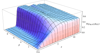
Figure 2: (Color online) Plot of the correlations of the Gibbs state (37) as a function of the inverse temperature $\beta$ and of the coupling constant $g$ according to Eq. (50). Parameters: $\omega=3$ and $\Delta=0.5$.

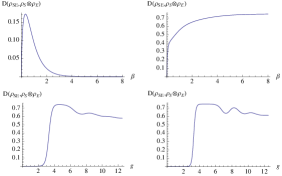
Figure 3: (Color online) (a, b, c, d From top left to bottom right) Sections of the plot in Fig. (2) corresponding to $g=1.7$, $g=5.5$ , $\beta=5$ and $\beta=8$, respectively. The critical value of $g$ is given by $\bar{g}_{1}=3.24$, see Eq. (51).

The above features can be explained considering that the trace distance $D(\rho_{SE},\rho_{S}\otimes\rho_{E})$ quantifies the correlations of the Gibbs state $\rho_{SE}$ and that the limit $\beta\rightarrow\infty$ corresponds to the limit of zero temperature, where the Gibbs state reduces to the ground state of the Hamiltonian $H$. If all the eigenvalues given by Eq. (40) are non-negative the ground state is $|\Phi^{-}_{0}\rangle=|0,0\rangle$ with eigenvalue zero. Of course, this is a product state and, therefore, the correlations of the Gibbs state approach zero for $\beta\to\infty$. This is what happens below the critical $g$. However, according to the level crossing described in Fig. (4), the Hamiltonian given by Eq. (20) has negative eigenvalues for larger values of the coupling constant $g$. In fact, it is easy to see from Eq. (40) that if

$$g>\bar{g}_{1}\equiv\sqrt{\omega^{2}+\omega\Delta}$$ (51)

then $E_{1}^{-}<0$ and, therefore, $|0,0\rangle$ is no longer the ground state. Thus, we can then identify $\bar{g}_{1}$ as the previously mentioned critical value of $g$, since for larger values the lowest energy state is $|\Phi^{-}_{1}\rangle$ which is an entangled state according to Eq. (38) with correlations $a_{1}^{2}b_{1}^{2}+a_{1}b_{1}$ different from zero. But looking at the dependence of the different eigenvalues $E_{n}^{-}$ on the coupling constant $g$, see Fig. (4), we can see that there is another critical point, let us call it $\bar{g}_{2}$, where $E^{-}_{2}(\bar{g}_{2})=E^{-}_{1}(\bar{g}_{2})$ and after which $E^{-}_{2}(g)<E^{-}_{1}(g)$, i.e., $|\Phi_{2}^{-}\rangle$ becomes the lowest energy state. We then have another value $\bar{g}_{3}$ for which $E^{-}_{3}(\bar{g}_{3})=E^{-}_{2}(\bar{g}_{3})$, so that for stronger couplings $|\Phi^{-}_{3}\rangle$ becomes the new ground state, and so on. Between two successive critical values $\bar{g}_{i}$ and $\bar{g}_{i+1}$ the ground state of the Hamiltonian is $|\Phi_{i}^{-}\rangle$, whose correlations according to Eq. (35) are given by

$$D\left(\rho_{SE},\rho_{S}\otimes\rho_{E}\right)=a_{i}^{2}b_{i}^{2}+a_{i}b_{i}=\frac{g^{2}}{\Delta^{2}+4g^{2}}+\sqrt{\frac{g^{2}}{\Delta^{2}+4g^{2}}}.$$ (52)

This expression characterizes the asymptotic value of the correlations in the Gibbs state for $\beta\to\infty$ and for $g$ between $\bar{g}_{i}$ and $\bar{g}_{i+1}$. We note that $D(\rho_{SE},\rho_{S}\otimes\rho_{E})$ approaches the value $\frac{3}{4}$ if we also let $g\to\infty$. As is shown in the Appendix, this asymptotic value corresponds in fact to the maximal possible value of the correlations for the present model.

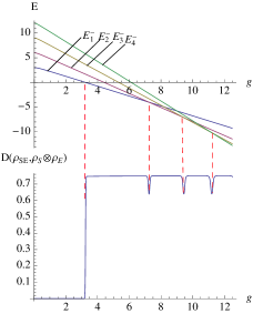
Figure 4: (Color online) (Top) Plot of the first energy eigenvalues $E^{-}_{1},E^{-}_{2},E^{-}_{3},E^{-}_{4}$ given by Eq. (40) as functions of $g$, $E^{-}_{0}$ coincides with the $x$-axis. (Bottom) Plot of the correlations of the Gibbs state as a function of $g$ for $\beta=100$, i.e., for approximately zero temperature; the other values are the same as in Fig. (2). The critical values of the correlations as a function of $g$ exactly correspond to the level crossing points: When $E^{-}_{0}=E^{-}_{1}$ there is a sudden increase and at the subsequent points the dips occur. For this value of $\beta$ the behavior described by the exact expression is well approximated by Eq. (52) between the dips and by Eq. (54) at the dips.

We see from Fig. (4) that for small temperatures the correlations in the Gibbs state exhibit a dip at every $\bar{g}_{i}$ with $i>1$. Again, this feature can be explained considering the ground level of the Hamiltonian given by Eq. (20). For $g=\bar{g}_{i}$ the eigenspace of the lowest energy level is two-fold degenerate since $E_{i}^{-}(\bar{g}_{i})=E_{i-1}^{-}(\bar{g}_{i})$ and the Gibbs state reduces to

$$\frac{1}{2}\left(|\Phi_{i-1}^{-}\rangle\langle\Phi^{-}_{i-1}|+|\Phi_{i}^{-}\rangle\langle\Phi^{-}_{i}|\right)$$ (53)

where, again we have ordered the elements of the basis as $\left\{|1,i-2\rangle,|0,i-1\rangle,|1,i-1\rangle,|0,i\rangle\right\}$. Equation (53) can be directly obtained from Eq. (LABEL:eq:gibbsmat), observing that for $\beta\rightarrow\infty$ the only non-negligible terms are those involving the exponentials of $\beta E^{-}_{i-1}$ or $\beta E_{i}^{-}$. Calculating now the corresponding product state and proceeding as done to obtain Eq. (50), or directly taking the limit of this equation for $\beta\rightarrow\infty$ and $g=\bar{g}_{i}$, one finds an explicit expression for the correlations of the mixed state given by Eq. (53):

$$D\left(\rho_{SE},\rho_{S}\otimes\rho_{E}\right)$$

$$=\frac{1}{2}\left[\alpha+\frac{1}{2}|\gamma_{1}+\delta_{1}+\sqrt{(\gamma_{1}-\delta_{1})^{2}+4\varepsilon^{2}_{1}}|\right.$$

$$\left.+\frac{1}{2}|\gamma_{1}+\delta_{1}-\sqrt{(\gamma_{1}-\delta_{1})^{2}+4\varepsilon^{2}_{1}}|\right.$$

$$+\frac{1}{2}|\gamma_{2}+\delta_{2}+\sqrt{(\gamma_{2}-\delta_{2})^{2}+4\varepsilon^{2}_{2}}|$$

$$\left.+\frac{1}{2}|\gamma_{2}+\delta_{2}-\sqrt{(\gamma_{2}-\delta_{2})^{2}+4\varepsilon^{2}_{2}}|+\chi\right],$$ (54)

where

$$\alpha=\frac{b_{i-1}^{2}}{4}\left(a_{i-1}^{2}+a_{i}^{2}\right);\,\,\,\,\gamma_{1}=\frac{b_{i-1}^{2}}{2}-\frac{b_{i-1}^{2}}{4}\left(b_{i-1}^{2}+b_{i}^{2}\right);$$

$$\delta_{1}=\frac{a_{i-1}^{2}}{2}-\frac{1}{4}\left(a_{i-1}^{2}+a_{i}^{2}\right)\left(a_{i-1}^{2}+b_{i}^{2}\right);\,\,\,\varepsilon_{1}=-\frac{a_{i-1}b_{i-1}}{2};$$

$$\gamma_{2}=\frac{b_{i}^{2}}{2}-\frac{1}{4}\left(b_{i-1}^{2}+b_{i}^{2}\right)\left(a_{i-1}^{2}+b_{i}^{2}\right);\,\,\,\,\varepsilon_{2}=-\frac{a_{i}b_{i}}{2};$$

$$\delta_{2}=\frac{a_{i}^{2}}{2}-\frac{a_{i}^{2}}{4}\left(a_{i-1}^{2}+a_{i}^{2}\right);\,\,\,\,\chi=\frac{a_{i}^{2}}{4}\left(b_{i-1}^{2}+b_{i}^{2}\right).$$ (55)

From the explicit evaluation of Eq. (52) and Eq. (54) for the different values of $i$, one can see that indeed the total amount of correlations of the mixed state given by Eq. (53) is smaller than the correlations of the dressed states $|\Phi_{i-1}^{-}\rangle$ and $|\Phi^{-}_{i}\rangle$ giving its decomposition, which explains the emergence of the dips. Note however that the correlation measure given by $D(\rho_{SE},\rho_{S}\otimes\rho_{E})$ is not a convex function on the space of physical states.

The above arguments are summarized in Fig. (4). They explain the behavior of the correlations in the Gibbs state for small temperatures, i.e., for $\beta\rightarrow\infty$. The effect of finite temperatures is to smoothen the dependence on $g$, as can be seen in Fig. (4), (3.d) and (3.c), such that the sudden increase at $g=\bar{g}_{1}$ is less sharp and that the subsequent dips turn into oscillations which are more and more suppressed as the temperature increases. This behavior is due to the fact that at finite temperature the Gibbs state has a non-vanishing admixture of $|\Phi^{-}_{1}\rangle$ for values of $g$ which are smaller than $\bar{g}_{1}$ and, hence, the increase of the correlations starts before $g=\bar{g}_{1}$ and is less sharp, as can be seen from Figs. (4) and (3.d). Moreover, as a consequence of finite temperatures, the Gibbs state is a mixed state even between the critical values $\bar{g}_{i}$, such that its correlations become smaller than in the zero temperature limit, which leads to a suppression of the oscillations.

III.3 Time evolution of the trace distance

The analysis performed so far concerns the correlations of the initial Gibbs state, i.e., the upper bound of the trace distance between the reduced state $\rho^{1}_{S}(t)$, evolving from an initial total Gibbs state, and the reduced state $\rho^{2}_{S}(t)$, evolving from the corresponding product state, according to Eq. (19). We will now investigate the dynamics of the trace distance $D(\rho^{1}_{S}(t),\rho^{2}_{S}(t))$ and analyze, in particular, the dependence of the supremum of this function on the coupling constant and the temperature. As discussed before (see Sec. II.1.2), the behavior of the trace distance between $\rho^{1}_{S}(t)$ and $\rho^{2}_{S}(t)$ expresses the effect of the initial correlations in the resulting dynamics. Moreover, its supremum as a function of time quantifies the amount of information which could not be initially retrieved by measurements on the reduced system only, but becomes accessible in the subsequent dynamics, thus making the two reduced states $\rho^{1}_{S}(t)$ and $\rho^{2}_{S}(t)$ more distinguishable.

Taking as initial state $\rho^{1}_{SE}$ the Gibbs state given by Eq. (37) and $\rho^{2}_{SE}$ as the corresponding product of its marginals, we have $\rho^{1}_{S}(t)=\rho^{1}_{S}(0)$ since the Gibb state is invariant under the time evolution, and $\rho_{S}^{1}(0)=\rho^{2}_{S}(0)$ because the corresponding open system initial states are identical. Thus, exploiting Eq. (45) we obtain the following explicit expression for the trace distance,

$$D(\rho^{1}_{S}(t),\rho^{2}_{S}(t)) = \left|\left(\rho_{00}-1\right)\sum_{n}(n+1)\rho^{nn}|d_{n+1}(t)|^{2}\right.$$ (56)

$$\left.+\rho_{00}\sum_{n}n\rho^{nn}|d_{n}(t)|^{2}\right|.$$

For fixed values of the parameters characterizing the dynamics this expression describes a superposition of periodic functions with incommensurable periods, i.e., an almost periodic function as already encountered in Sec. II.2. An example for the trace distance dynamics is shown in Fig. (5). The trace distance starts growing already at the initial time and further oscillates with time, according to the almost periodic behavior described by Eq. (56).

Figure 5: (Color online) The trace distance $D(\rho^{1}_{S}(t),\rho^{2}_{S}(t))$ as a function of time according to Eq. (56); $\rho^{i}_{S}(t)$ is the state of the reduced system at time $t$ obtained from an initial total state $\rho^{i}_{SE}$, where $\rho^{1}_{SE}$ is the Gibbs state given by Eq. (37) and $\rho^{2}_{SE}$ is the corresponding product state. The upper horizontal line represents the bound given by the right-hand side of the inequality (19) which has been determined by Eq. (50). Parameters: $\omega=3$, $\Delta=0.5$, $g=6$ and $\beta=5$.

As mentioned already the time dependence of the trace distance is solely due to the time evolution of the product state constructed from the marginals of the Gibbs state since the latter is invariant under the dynamics. It is the comparison between the two different reduced system states, namely between the states $\rho^{1}_{S}(t)=\rho^{1}_{S}(0)$ and $\rho^{2}_{S}(t)$, which allows to obtain information initially not accessible with measurement on the reduced system only, and which enables the detection of correlations in the initial Gibbs state.

The supremum of the trace distance in Fig. (5) is substantially smaller than the corresponding bound of Eq. (19). For large values of $\beta$ and $g$ the supremum can be estimated as follows. If the temperature goes to zero the Gibbs state approaches the projection onto the ground state which is given by $|\Phi^{-}_{k}\rangle\langle\Phi^{-}_{k}|$ for a fixed $k$, depending on the value of the coupling constant $g$. We suppose that $g$ is different from the critical values $\bar{g}_{i}$. This implies $\rho_{00}=a_{k}^{2}$, $\rho_{11}=b_{k}^{2}$, together with $\rho^{mm}=\delta_{m,k}a_{k}^{2}+\delta_{m,k-1}b_{k}^{2}$. For large values of $g$, which implies large values of $k$, we have $a_{k}\approx b_{k}\approx{1}/{\sqrt{2}}$. Employing further Eq. (23), one thus obtains the estimate

$$D(\rho^{1}_{S}(t),\rho^{2}_{S}(t))\approx\frac{1}{4}\left|\sin(2\sqrt{k}gt)\sin(gt/\sqrt{k})\right|.$$ (57)

This shows that for large $\beta$ and $g$ the trace distance is bounded from above by $\frac{1}{4}$.

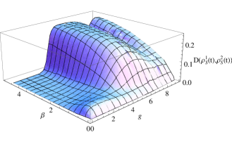
Figure 6: (Color online) The supremum of $D(\rho^{1}_{S}(t),\rho^{2}_{S}(t))$ as a function of time versus the coupling constant $g$ and the inverse temperature $\beta$; $\rho^{1}_{S}(t)$ is obtained from an initial total Gibbs state, $\rho_{S}^{2}(t)$ from the corresponding product state, $D(\rho^{1}_{S}(t),\rho^{2}_{S}(t))$ is calculated according to Eq. (56). Parameters: $\omega=3$, $\Delta=0.5$.

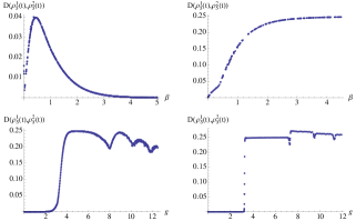
Figure 7: (Color online) (a, b, c, d From top left to bottom right) The same as Fig. (6) but for parameters $g=1.7$, $g=5.5$, $\beta=5$ and $\beta=100$, respectively. For $\beta=100$, i.e., approximately zero temperature, the dips occur at the same values as the corresponding dips of the bound, see Fig. (4). For the case of finite temperature the dips are not suppressed, but they are shifted towards larger values of $g$.

Figure (6) shows how the supremum of $D(\rho^{1}_{S}(t),\rho^{2}_{S}(t))$ behaves as a function of the coupling constant $g$ and the inverse temperature $\beta$, keeping fixed $\omega$ and $\Delta$. Exactly as for the correlations of the Gibbs state [compare with Fig. (2)], we observe two qualitatively different kinds of behavior as a function of $\beta$, for a fixed value of $g$. Below a critical $g$ the supremum of the trace distance passes through maximum and then tends to zero; above the critical value it tends monotonically to an asymptotic value which is close to the estimate of $\frac{1}{4}$ determined above, as illustrated in Figs. (7.a) and (7.b). Moreover, considering the supremum of the trace distance as a function of $g$ for fixed $\beta$, after a sudden growth at the first critical $g$ it exhibits some oscillations analogous to those of the bound. Comparing Figs. (4) and (7), we see that in the limit of zero temperature the bound and the true supremum of the trace distance both show a sudden increase and subsequent dips at the same values of the coupling constant $g$. This behavior can be explained by recalling the dependence of the energy spectrum of the Hamiltonian as a function of $g$ in Fig. (4). At zero temperature the Gibbs state reduces to the ground level of the Hamiltonian. The discontinuous change in the ground level with varying $g$, i.e. the transition from $|\Phi_{i}\rangle$ to $(|\Phi_{i}\rangle+|\Phi_{i+1}\rangle)/\sqrt{2}$, implies a discontinuous change in the bound as well as in the supremum of the trace distance, thus leading to the dips appearing in Fig. (4) and Fig. (7). In fact, apart from fixing the bound at the r.h.s. of Eq. (19), the Gibbs state determines both reduced states $\rho^{1}_{S}(t)$ and $\rho^{2}_{S}(t)$, arising from the initial total states $\rho_{SE}$ and $\rho_{S}\otimes\rho_{E}$ respectively. Relying on Eq. (27) one can see that for $\Delta=0$ the supremum of the trace distance is simply given by 1/4 for an initial correlated state $\rho_{SE}=|\Phi_{i}\rangle\langle\Phi_{i}|$, for any $i>0$. This means that for zero detuning the supremum of the trace distance dynamics as a function of $g$ at zero temperature takes the constant value $1/4$, except at $g=\bar{g}_{i}$ where the dips occur. The effect of a finite temperatures is slightly different for the bound and the supremum of the trace distance dynamics: With growing temperature the dips of the bound turn into oscillations which are more and more suppressed, but they occur at the same values of $g$. On the contrary, the dips of the true supremum, and its sudden increase as well, are not suppressed, but do change position, occurring at larger values of $g$.

IV Conclusions

We have studied the influence of initial correlations between system and reservoir on the dynamics of an open quantum system by means of the trace distance, considering the paradigmatic and exactly solvable model provided by the Jaynes-Cummings Hamiltonian. First, we have analyzed the amount of correlations in the Gibbs state $\rho_{SE}$ as it is quantified by $D(\rho_{SE},\rho_{S}\otimes\rho_{E})$, where $\rho_{S}\otimes\rho_{E}$ denotes the product state arising from the marginals of $\rho_{SE}$. The exact analytical expression of the latter quantity describes a non-monotonic behavior as a function of both the coupling constant and the temperature characterizing the dynamics. The same behavior is found for the supremum of the trace distance between the open system states $\rho^{1}_{S}(t)$ and $\rho^{2}_{S}(t)$ which evolve from $\rho_{SE}$ and $\rho_{S}\otimes\rho_{E}$, respectively. This enabled us to establish a clear connection between the correlation properties of the Gibbs state and basic features of the subsequent open system dynamics, in particular, the amount of information which is initially inaccessible for the open system and which is uncovered during its time evolution. The dynamical behavior of the trace distance between the reduced system states $\rho^{1}_{S}(t)$ and $\rho^{2}_{S}(t)$ thus provides a witness for the correlations of the total system’s initial state.

As we have shown for the case at hand, at zero temperature sudden changes in the supremum over time of the trace distance can be traced back uniquely to discontinuous changes in the structure of the total system’s ground state and to its degree of entanglement which, in turn, is caused by crossings of the energy levels of the total system Hamiltonian. It is important to remark that, as we have demonstrated, clear signatures of these discontinuities are still present at finite temperatures. Note that to reconstruct the trace distance dynamics, in order to detect correlation properties of the ground state, one only needs to follow the evolution of the open system state obtained from the initial total product state $\rho_{S}\otimes\rho_{E}$.

The bound given by the right-hand side of Eq. (19) is able to represent qualitatively the non-trivial behavior of the maximum of the trace distance between $\rho^{1}_{S}(t)$ and $\rho^{2}_{S}(t)$, as a function of the different parameters characterizing the Hamiltonian and the temperature. While for the sudden transition between the two different asymptotic regimes as a function of $\beta$ it is clear that the effective maximum of $D(\rho^{1}_{S}(t),\rho^{2}_{S}(t))$ has to reproduce the behavior of the bound, it is quite remarkable that also in the second case, where the bound is sensibly different from the effective maximum and from zero, both these quantities show an analogous non-monotonic behavior. Finally, we note that it must be expected that the general features found here for the correlated Gibbs state hold true also for other correlated initial states, e.g., for correlated non-equilibrium stationary states, as long as the latter involve discontinuous, qualitative changes under the variation of some system parameters.

*

Appendix A General bound for the correlations of a quantum state

Throughout the article we have used the quantity $D(\rho_{SE},\rho_{S}\otimes\rho_{E})$ as a measure for the total amount of correlations of given state $\rho_{SE}$. On the ground of extensive numerical simulations we conjecture that this quantity satisfies the inequality

$$D(\rho_{SE},\rho_{S}\otimes\rho_{E})\leq 1-\frac{1}{N^{2}},$$ (58)

where $N$ denotes the minimum of the dimensions of $\mathcal{H}_{S}$ and $\mathcal{H}_{E}$. For the example studied in this paper we have $N=2$ and, hence, $D(\rho_{SE},\rho_{S}\otimes\rho_{E})\leq\frac{3}{4}$.

To our knowledge there exists no general mathematical proof for the inequality (58). However, one can easily prove that this inequality is saturated if $\rho_{SE}=|\psi\rangle\langle\psi|$ is a pure, maximally entangled state. To show this we first note that for a maximally entangled state vector $|\psi\rangle$ the marginal states are given by $\rho_{S}=P_{S}/N$ and $\rho_{E}=P_{E}/N$, where $P_{S}$ and $P_{E}$ are the projections onto the subspaces of $\mathcal{H}_{S}$ and $\mathcal{H}_{E}$, respectively, which are spanned by the local Schmidt basis vectors with nonzero Schmidt coefficients. Hence, $D(\rho_{SE},\rho_{S}\otimes\rho_{E})$ is given by $\frac{1}{2}$ times the sum of the absolute eigenvalues of the operator

$$X=|\psi\rangle\langle\psi|-\frac{1}{N^{2}}P_{S}\otimes P_{E}.$$ (59)

Obviously, $|\psi\rangle$ is an eigenvector of $X$ corresponding to the eigenvalue $1-1/N^{2}$. Moreover, all vectors which are perpendicular to $|\psi\rangle$ and belong to the support of $P_{S}\otimes P_{E}$ are eigenvectors of $X$ with the eigenvalue $-1/N^{2}$. Thus, $X$ has one non-degenerate eigenvalue $1-1/N^{2}$, and one eigenvalue $-1/N^{2}$ which is $(N^{2}-1)$-fold degenerate, while all other eigenvalues of $X$ are zero. Therefore we have

$$D(\rho_{SE},\rho_{S}\otimes\rho_{E})=\frac{1}{2}\left[1-\frac{1}{N^{2}}+(N^{2}-1)\frac{1}{N^{2}}\right]=1-\frac{1}{N^{2}},$$ (60)

which proves the claim.

References

- (1) H.-P. Breuer and F. Petruccione, The Theory of Open Quantum Systems (Oxford University Press, Oxford, 2007).
- (2) V. Gorini, A, Kossakowski, and E. C. G. Sudarshan, J. Math. Phys. 17, 821 (1976).
- (3) G. Lindblad, Comm. Math. Phys. 48, 119 (1976).
- (4) S. Daffer, K. Wódkiewicz, J. D. Cresser, and J. K. McIver, Phys. Rev. A 70, 010304 (2004).
- (5) A. A. Budini, Phys. Rev. A 69, 042107 (2004).
- (6) A. Shabani and D. A. Lidar, Phys. Rev. A 71, 020101 (2005).
- (7) S. Maniscalco and F. Petruccione, Phys. Rev. A 73, 012111 (2006).
- (8) B. Vacchini, Phys. Rev. A 78, 022112 (2008).
- (9) E. Ferraro, H.-P. Breuer, A. Napoli, M. A. Jivulescu, and A. Messina, Phys. Rev. B 78, 064309 (2008).
- (10) A. Kossakowski and R. Rebolledo, Open Syst. Inf. Dyn. 15, 135 (2008).
- (11) A. Kossakowski and R. Rebolledo, Open Syst. Inf. Dyn. 16, 259 (2009).
- (12) H.-P. Breuer and B. Vacchini, Phys. Rev. Lett. 101, 140402 (2008).
- (13) H.-P. Breuer and B. Vacchini, Phys. Rev. E 79, 041147 (2009).
- (14) J Piilo, S. Maniscalco, K. Härkönen, and K.-A. Suominen, Phys. Rev. Lett. 100, 180402 (2008).
- (15) J. Piilo, K. Härkönen, S. Maniscalco, and K.-A. Suominen, Phys. Rev. A 79, 062112 (2009).
- (16) H.-P. Breuer and J. Piilo, Europhys. Lett. 85, 50004 (2009).
- (17) H.-P. Breuer, E.-M. Laine, and J. Piilo, Phys. Rev. Lett. 103, 210401 (2009).
- (18) E.-M. Laine, J. Piilo, and H.-P. Breuer, Phys. Rev. A 81, 062115 (2010).
- (19) B. Vacchini and H.-P. Breuer, Phys. Rev. A 81, 042103 (2010).
- (20) A. Smirne and B. Vacchini, Phys. Rev. A in press (2010).
- (21) D. Chruściński and A. Kossakowski, Phys. Rev. Lett. 104, 070406 (2010).
- (22) D. Chruściński, A. Kossakowski, and S. Pascazio, Phys. Rev. A 81, 032101 (2010).
- (23) L. Mazzola, E.-M. Laine, H.-P. Breuer, S. Maniscalco, and J. Piilo, Phys. Rev. A 81, 062120 (2010).
- (24) P. Pechukas, Phys. Rev. Lett. 73, 1060 (1994).
- (25) R. Alicki, Phys. Rev. Lett. 75, 3020 (1995).
- (26) C. Uchiyama and M. Aihara, Phys. Rev. A. 82, 044104 (2010).
- (27) A. Smirne and B. Vacchini, Phys. Rev. A 82, 022110 (2010).
- (28) A. J. van Wonderen and K. Lendi, J. Phys. A: Math. Gen. 33, 5757 (2000).
- (29) P. Štelmachovič and V. Bužek, Phys. Rev. A 64, 062106 (2001).
- (30) T. F. Jordan, A. Shaji, and E. C. G. Sudarshan, Phys. Rev. A 70, 052110 (2004).
- (31) C. A. Rodríguez-Rosario, K. Modi, A. Kuah, A. Shaji, and E. C. G. Sudarshan, J. Phys. A: Math. Gen. 41, 205301 (2008).
- (32) H. A. Carteret, D. R. Terno, and K. Życzkowski, Phys. Rev. A 77, 042113 (2008).
- (33) A. Shabani and D. A. Lidar, Phys. Rev. Lett. 102, 100402 (2009).
- (34) E.-M. Laine, J. Piilo, and H.-P. Breuer (2010), arXiv:1004.2184 [quant-ph].
- (35) J. Dajka and J. Łuczka, Phys. Rev. A 82, 012341 (2010).
- (36) M. B. Ruskai, Rev. Math. Phys. 6, 1147 (1994).
- (37) A. Gilchrist, N. K. Langford, and M. A. Nielsen, Phys. Rev. A 71, 062310 (2005).
- (38) R. R. Puri, Mathematical Methods of Quantum Optics (Springer, Berlin, 2001).
- (39) C. Corduneanu. Almost Periodic Functions (Chelsea Publishing Company, New York, 1989).
- (40) Due to the incommensurability of the frequencies, there is no time at which attains the supremum.
- (41) P. Meystre and M. Sargent III. Elements of Quantum Optics (Springer-Verlag, Berlin, 1991).