The Locality Problem in Quantum Measurements

 

The locality problem of quantum measurements is considered in the framework of the algebraic approach. It is shown that contrary to the currently widespread opinion one can reconcile the mathematical formalism of the quantum theory with the assumption of the existence of a local physical reality determining the results of local measurements. The key quantum experiments: double-slit experiment on electron scattering, Wheeler’s delayed-choice experiment, the Einstein-Podolsky-Rosen paradox, and quantum teleportation are discussed from the locality-problem point of view. A clear physical interpretation for these experiments, which does not contradict the classical ideas, is given.

Department of Physics, Moscow State University,
Moscow 119899, Russia. E-mail: slavnov@goa.bog.msu.ru

PACS: 03.65.Ud

1 INTRODUCTION

The locality problem is one of the main problems in the entire quantum theory. It attracted especially close attention during the construction of the quantum field theory (see, e.g., [2, 3, 4, 5]), where the locality axiom plays a central role. This axiom has different formulations; however, without going into mathematical subtleties, it can be reduced to the following: boson fields must commute at space-like separated points, while fermion fields must anti-commute. If the dynamics of a quantum system is described by a Lagrangian, it is additionally required that this Lagrangian must be a local function of the fields.

The following argument is often used as a physical justification of the locality axiom. The results of the measurement in a bounded domain of a Minkowski space (a local measurement) are determined by boson-field values and by bilinear combinations of fermion fields in this domain.

Such locality requirement is purely mathematical in its nature. It can be formulated only in the framework of a particular mathematical formalism, and it is a part of that formalism. In a general discussion of locality it is desirable to proceed from requirements that can be formulated in physics terminology and that can be checked in the experiment directly. Such formulation is fairly obvious.

If two bounded domains ${\cal O}_{1}$ and ${\cal O}_{2}$ of the Minkowski space are space-like separated, then the results of measurements in the domain ${\cal O}_{1}$ do not depend on any manipulations in the ${\cal O}_{2}$.

At this point one has to make the following warning. The above requirement does not imply that the measurement results in the domains ${\cal O}_{1}$ and ${\cal O}_{2}$ may not be related to each other. This of course is not true. Such measurement results may have a common cause, and therefore, a correlation between them is quite possible.

Practically no one argues with the above formulation. However, the situation changes radically when we try to supplement the above requirement with the following one. There exists a certain physical reality, which determines the results of a local measurement.

Many people object to such an extension of the locality requirement. The arguments on this matter began a long time ago. One can recall the famous debates between Einstein and Bohr. Einstein (see [6, 7, 8]) was in favor of the above extension, while Bohr (see [9, 10]) was against it.

Later on, the majority’s opinion within the physics scientific community leaned towards the Bohr side. The results of many modern experiments related to this problem are currently considered as proof that the physical reality mentioned above does not exist. Or, at least, the assumption of the existence of such a reality contradicts the accepted mathematical formalism of the quantum theory.

However, if we abandon the extension formulated above, we almost completely lose the physical foundation behind the locality axiom accepted in the quantum field theory. This rejection would force us to assume that neither local fields, nor their combinations describe a local reality (because it does not exist). Then, it is not clear why these combinations must commute in space-like separated domains.

Thus we have a deadlock situation. The assumption of the existence of a local physical reality contradicts the mathematical formalism of the quantum theory. At the same time, the rejection of this assumption denies the physical foundation one of the main axioms in the mathematical formalism of the quantum field theory. Of course, one can abandon attempts of any physical justification of the locality axiom. This would affect neither the logical nor mathematical structure of the quantum theory. However, from the physical point of view this way out of the uncomfortable situation is extremely undesirable.

In the present paper we will attempt to demonstrate that the mathematical formalism accepted within the quantum theory is quite compatible with the assumption of the existence of physical reality determining the results of local measurements. The often-produced incompatibility proofs have the following two flaws. First, these proofs often point out toward a contradiction between the experimental data and certain mathematical assumptions, which are used in the construction of mathematical formalism. However, the questions of physical validity of these assumptions and their necessity are usually not discussed. Second, the interpretation given to the obtained experimental data is far from being always adequate.

The so-called de Broglie waves [11] can be considered as one of the most striking examples of inadequate interpretation. In the beginning of practically any textbook on quantum mechanics it is said that a de Broglie wave with the wavelength

$$\lambda=\frac{2\pi\hbar}{k}.$$ (1)

is associated with any quantum particle having the momentum $k$. The results of electron diffraction experiments [12, 13], or the later results on the electron interference [14]. are mentioned as examples supporting the above statement. In agreement with (1) a clear interference pattern was observed in the latter experiment.

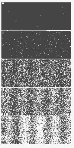
Figure 1: Interference pattern in electron scattering.

Equation (1) became the basis of subsequent assertions, that the distinctive feature of quantum particles is the presence of both corpuscular and wave properties. These assertions seem to be quite well supported experimentally. Nevertheless, we would like to examine if this is indeed the case.

Let us turn to the results of more recent experiments performed by Tonomura [15, 16]. These experiments investigated electron beam scattering by a biprism, which by its physical properties is analogous to a double-slit screen. The beam intensity was so low, that on average there was less than one electron in the experimental apparatus at any single moment. This allowed one to neglect the influence of inter-electron interaction on the results of the experiment. Moreover, it was possible to register the results of passage of a small number of electrons in this experiment.

The experimental results are shown in Fig. 1, reprinted from the review [16]. The individual photographs correspond to different exposure times. The photograph (a) registered traces of 10 electrons, the photograph (b) 200 electrons, the photograph (c) 6000 electrons, the photograph (d) 40000 electrons, and the photograph (e) 140000 electrons.

We see that when only a small number of electrons are registered (the photographs (a) and (b)) the interference pattern is not showing through. Such a pattern appears only after a very large number of electrons were registered (the photographs (d) and (e)). If we try to determine the electron wavelength with a help of the photographs (a) and (b), we do not obtain anything similar to (1).

These results speak in favor of the fact that wave properties are not revealed by a single electron. They become apparent only in a specially prepared ensemble of electrons. In the considered case, all electrons had approximately the same momentum.

Now we can look at Eq. (1) in a new light. We can assume that it is relevant not to a single electron, but to a specially prepared ensemble of electrons. At this point it is appropriate to say that Blokhintsev [17, 18, 19, 20] was a passionate supporter of the view that most of the quantum mechanics formulas are relevant not to isolated quantum particles, but to their ensembles. This novel point of view on the connection between momentum and spatial characteristics of quantum objects might prove to be very important for discussions of the locality properties. The localization domain of a single object is one thing, but the localization domain of an ensemble of these objects is an entirely different story. Later on we will come back to discussion of this question.

The commonly used in textbooks formulation of the mathematical formalism of the quantum theory, with wave functions or state vectors as the basic elements, is not ideal for discussions of the locality problem, because these objects themselves are obviously nonlocal. The so-called algebraic approach [21, 22, 23] is much better suited for these purposes. Unlike the traditional

approach, the Hilbert’s space of state vectors is no longer a primary object of the theory within the algebraic approach, and observables are no longer defined as operators in the Hilbert space.

Observables, more specifically, local observables are considered as the primary elements of the theory. Heuristically, an observable is defined as such an attribute of the investigated physical system for which one can obtain some numerical value with the help of a certain measuring procedure. Accordingly, for local observables one can obtain numerical values with the help of local measurements. Usually it is assumed that some unit system is chosen, and therefore one can consider all observables as dimensionless.

Initially the observables are not related to operators in a Hilbert space at all. The Hilbert space itself is constructed with the help of observables as some secondary object. After that a connection between the observables and the operators in this space is established.

We will conduct the subsequent examination in the framework of a special version of the algebraic approach previously described in detail in the paper [24]. A more concise description can be found in the papers [25, 26]. In the papers [24, 25] the theory was constructed using an inductive approach, where physical laws are noticed first, and then they are formulated as mathematical axioms. In the present paper we will use a deductive approach, where the main axioms are formulated from the very beginning. We refer the readers wishing to get acquainted with physical justifications of these axioms to the paper [24]. The main definitions and statements from the theory of algebras can be found in the same paper.

2 THE MAIN ASPECTS OF THE ALGEBRAIC
APPROACH

We begin from stating the basic properties of observables. The main property is the following one. The observables can be multiplied by real numbers, added to each other, and multiplied by one another. This property is formulated as the following postulate.

Postulate 1. The observables $\hat{A}$ of a physical system are Hermitian elements of some $C^{*}$-algebra.

Postulate 1 (and all the subsequent ones) is valid for classical systems as well. We remind the reader that algebra is a set of elements, which, firstly, is a linear space; secondly, a multiplication operation is defined for pairs of elements from that set. That is, for any two elements $\hat{U},\hat{V}\in\hbox{\gotb A}$ a third element $\hat{W}\in\hbox{\gotb A}$ is assigned, and the following notation is used $\hat{W}=\hat{U}\hat{V}$. This assignment satisfies a number of properties, which are standard for multiplication operations. An algebra A is a $C^{*}$-algebra (see, e.g., [27]), if a conjugation operation (involution) $\hat{U}\to\hat{U}^{*}$ $(\hat{U}\in\hbox{\gotb A},\quad\hat{U}^{*}\in\hbox{\gotb A})$ is defined on A, and the norm of any element $\hat{U}$ satisfies the condition $\|\hat{U}\hat{U}^{*}\|=\|\hat{U}\|^{2}$. The justification why the algebra A must be a $C^{*}$ algebra can be found in [24]. An element $\hat{U}$ is called Hermitian, if $\hat{U}^{*}=\hat{U}$. The set of observables will be denoted $\hbox{\gotb A}_{+}$ ($\hbox{\gotb A}_{+}\subset\hbox{\gotb A}$). In classical systems all observables are compatible with each other (can be measured simultaneously). In a quantum system they can be either compatible or incompatible.

Postulate 2. The set of compatible with each other observables is a maximal real associative commutative subalgebra $\hbox{\gotb Q}_{\xi}$ of the algebra A ($\hbox{\gotb Q}_{\xi}\subset\hbox{\gotb A}_{+}$).

The index $\xi$, which runs through the set $\Xi$, distinguishes one such subalgebra from another. For a classical system the set $\Xi$ contains just a single element, for a quantum system $\Xi$ contains infinitely many elements.

Of course, in the framework of the traditional approach to the quantum theory, the bounded observables satisfy Postulates 1 and 2. However, there is an additional requirement within the traditional approach, that the observables are described by self-adjoint operators defined in a Hilbert space. This requirement allows one to construct a very efficient mathematical formalism; however, it does not have an intuitive physical foundation. Moreover, the necessity of this additional requirement is not quite clear.

The set of observables $\hbox{\gotb A}_{+}$ can be considered as a mathematical model of a quantum system. Accordingly, the subset $\hbox{\gotb Q}_{\xi}$ can be considered as observables of some classical subsystem. This subsystem is open, because the quantum-system’s degrees of freedom corresponding to observables from different subsets $\hbox{\gotb Q}_{\xi}$ can interact with each other.

Moreover, these classical subsystems may not have their own dynamics, because the generalized coordinates and momenta corresponding to the same degree of freedom, may belong to different subsets of $\hbox{\gotb Q}_{\xi}$. Therefore, the traditional approach for defining the state as a point of a phase space is not suitable for such subsystems. But, specifying a point in the phase space is equivalent to setting initial conditions for the equations of motion. This allows one to fix the values of all observables of the considered system. However, one can avoid using equations of motion and the initial condition, and fix the values of all observables directly. Such an approach is suitable for open systems as well.

Measuring the sum of observables in any concrete classical system yields the sum of the values of the individual observables, and measuring the product of observables yields the product of their individual values. In other words, specifying the values of all observables is equivalent to specifying some homomorphic map of the algebra of observables into the set of real numbers. For commutative associative algebra, such a map is called a character (see, e.g., [27]). Therefore we accept the following postulate.

Postulate 3. The state of a classical subsystem, whose observables are elements of a subalgebra $\hbox{\gotb Q}_{\xi}$, is described by a character of this subalgebra.

This definition of the state of a classical subsystem has an important advantage, that it can be generalized to the quantum case. Each quantum observable belonging to $\hbox{\gotb A}_{+}$, simultaneously belongs to some subalgebra $\hbox{\gotb Q}_{\xi}$. This allows one to consider a quantum system as a family of classical subsystems. If we knew the states of all these subsystems, we could have predicted the result of measuring any observable of the quantum system. This gives us grounds for accepting the following postulate.

Postulate 4. The result of measuring any observable of a quantum system is determined by its elementary state $\varphi$.

Here, $\varphi$ is a family $\varphi=[\varphi_{\xi}]$ of characters $\varphi_{\xi}$ of all subalgebras $\hbox{\gotb Q}_{\xi}$. Each subalgebra $\hbox{\gotb Q}_{\xi}$ in the family is represented by a single character.

At first it may seem that the last postulate contradicts the fact that one cannot predict the measurement results for all observables of a quantum system. However, there is no contradiction here. The point is that we can measure simultaneously (that is in a compatible way) only compatible observables. These observables belong to a certain subalgebra $\hbox{\gotb Q}_{\xi}$. Lets say for instance they belong to the subalgebra with the index $\xi=\eta$. Then, from the complete set $[\varphi_{\xi}]$ we can specify only one character $\varphi_{\eta}$. Endowed with such information we can predict only the measurement results for observables belonging to $\hbox{\gotb Q}_{\eta}$.

We will not be able to say anything certain about the values of other observables. Additional measurements, if they are not compatible with the previous ones, will not improve the situation. They will produce new information about the quantum system; however, simultaneously the additional measurements will disturb the state of our system and will make the information obtained earlier worthless.

Figuratively speaking, an elementary state is a holographic image of the system under investigation. Using classical measuring devices we can look at it from one side only, and, hence, obtain a two-dimensional image. Moreover, the measurement will disturb the system and will change its original holographic image. Therefore, if later we will look at the system from another side, we will see a two-dimensional projection of the new holographic image. Thus, we will never be able to see the entire holographic image.

Using the notion of an elementary state, one can see the Everett idea [28] on the existence of many parallel worlds in a new light. According to his original idea quantum systems simultaneously occupy many parallel worlds, while a classical observer lives in only one of these worlds chosen accidentally. Therefore, he sees only the version of the quantum system represented in his world. In this form the Everett idea looks implausible.

On the contrary, the idea that an elementary state is analogous to a holographic image looks quite plausible. On the other hand, the notion of an elementary state leads to roughly the same consequences as the idea of the existence of many worlds. However, there is an important difference. In Everett’s picture the randomness inherent to quantum measurements is connected with an accidental occupation of one or another world by the classical observer. In the language of probability theory, in this case, we are dealing with an ensemble of observers. When we describe a quantum system with the help of an elementary state, we obtain an incomplete description of the system. Therefore, in reality we describe not an individual system, but certain characteristics common for an entire ensemble of quantum systems.

In connection with the above it is useful to introduce the notion of $\varphi_{\eta}$-equivalence. Two elementary states $\varphi=[\varphi_{\xi}]$ $\varphi^{\prime}=[\varphi_{\xi}^{\prime}]$ will be called $\varphi_{\eta}$-equivalent, if $\varphi_{\eta}=\varphi^{\prime}_{\eta}$. The relations between the remaining characters $\varphi_{\xi}$ and $\varphi_{\xi}^{\prime}$ can be arbitrary. The class of $\varphi_{\eta}$-equivalent elementary states will be denoted $\{\varphi\}_{\varphi_{\eta}}$. The most that one can possibly learn about an elementary state $\varphi$ is that it belongs to some equivalence class $\varphi\in\{\varphi\}_{\varphi_{\eta}}$.

There is one more obstacle preventing unambiguous predictions of measurement results. One and the same observable $\hat{A}$ may belong simultaneously to several subalgebras $\hbox{\gotb Q}_{\xi}$: $\hat{A}\in\hbox{\gotb Q}_{\xi}\cap\hbox{\gotb Q}_{\xi^{\prime}}$ $(\xi\neq\xi^{\prime})$. Therefore, it is not clear which of the functionals (characters) $\varphi_{\xi}$ or $\varphi_{\xi^{\prime}}$ will describe the results of a particular measurement.

At first it may seem that this additional ambiguity can be easily eliminated with the help of the additional condition

$$\varphi_{\xi}(\hat{A})=\varphi_{\xi^{\prime}}(\hat{A}),\mbox{ }\hat{A}\in\hbox{\gotb Q}_{\xi}\cap\hbox{\gotb Q}_{\xi^{\prime}}.$$ (2)

However, this condition leads to numerous contradictions. Additional details can be found in the paper [24]. On the other hand, as was shown in the same paper [24], the condition (2) is not a necessary one. Indeed, the measurement result may depend not only on the system under investigation, but on the characteristics of the measuring device as well. From the observer’s point of view such dependence is extremely objectionable, and experimentalists try to minimize it as much as possible.

We have come to think that measurement results are virtually independent of the characteristics of ”good” measuring devices. However, for this to be true all the devices used for measuring the observable of interest must at least be calibrated in a consistent way. It was shown in [24] that the existence of incompatible measurements in the quantum case makes such calibration far from being always possible. In particular, if we assign a certain type of measuring devices ($\xi$-type) to every subalgebra $\hbox{\gotb Q}_{\xi}$, then, as it turns out, the devices of different types cannot be calibrated consistently. Therefore, one cannot get rid of a possible dependence of the measurement results on the device type (or, on the index $\xi$).

The above assertion does not exclude that for some elementary states $\varphi$ Eq. (2) will be valid for all $\hbox{\gotb Q}_{\xi}$, $\hbox{\gotb Q}_{\xi^{\prime}}$, containing the observable $\hat{A}$. In this case we shall say that the elementary state $\varphi$ is stable with respect to the observable $\hat{A}$.

Let us go back to the discussion of elementary states and of their equivalence classes. Measurements allow one to establish that the elementary state $\varphi$ of the system under investigation belongs to some equivalence class $\varphi\in\{\varphi\}_{\varphi_{\eta}}$. Thereafter, we can make the following predictions. Measuring devices of the $\eta$-type will yield the value $A=\varphi_{\eta}(\hat{A})$ for the observable $\hat{A}\in\hbox{\gotb Q}_{\eta}$. From now on the measurement result is denoted by the same symbol as the observable itself, but without the ”hat.” If the elementary state $\varphi$ is stable with respect to the observables $\hat{A}\in\hbox{\gotb Q}_{\eta}$, then the same result will be obtained by using measuring devices of any type $\xi$. Of course, the type $\xi$ must be such that $\hat{A}\in\hbox{\gotb Q}_{\xi}$, otherwise the device is simply not suitable for measuring the values of this observable. One cannot say anything definite about measurement results for observables $\hat{A}\notin\hbox{\gotb Q}_{\eta}$, because we will obtain different values for different elementary states $\varphi\in\{\varphi\}_{\varphi_{\eta}}$, .

Within the standard mathematical formalism of quantum mechanics all the physical properties mentioned above are exhibited by quantum states specified by particular values of a complete set of commuting observables. This allows one to state the following definition of a quantum state within the proposed approach.

Definition. A quantum state $\Psi_{\varphi_{\eta}}$ is the class $\{\varphi\}_{\varphi_{\eta}}$  $\varphi_{\eta}$- equivalent elementary states, which are stable with respect to the observables $\hat{A}\in\hbox{\gotb Q}_{\eta}$.

It is usually assumed that a quantum state $\Psi_{\varphi_{\eta}}$ appears as a result of measuring the observables $\hat{A}\in\hbox{\gotb Q}_{\eta}$, where a specified value is registered for each of the observables $\hat{A}$. Of course, this is not always true, at least, because some particles of the investigated system can be absorbed by the device in the measuring process. In order for a measurement to be simultaneously a preparation of a quantum state, it must be reproducible. If repeated measurements of an observable $\hat{A}$ give identical results, we shall mean the measurements reproducible. Note that the repeated measurements are not necessarily performed by measuring devices of the same type.

The paper [24] shows that quantum states defined above are always pure. Within the standard mathematical formalism of quantum mechanics pure states are defined as vectors $|\Phi\rangle$ of some Hilbert space H. These vectors are used for calculating the average values of observables in the corresponding quantum states. This definition works very well for applied purposes; however, it does not have an intuitively clear physical interpretation. Within the approach proposed in the present paper the average value of an observable is connected in a natural way with the probability distribution of the elementary states $\varphi$ within the equivalence class $\varphi\in\{\varphi\}_{\eta}$.

One has to bear in mind that the elementary states satisfy the standard properties of elementary events from the classical Kolmogorov probability theory [29]. Namely, each random experiment results in one and only one elementary event. Different elementary events are mutually exclusive. Note that the standard approach to quantum mechanics does not have such an ingredient. This became an insurmountable obstacle for application of the classical probability theory to quantum mechanics. Such an obstacle is absent within the approach used here. Therefore, there is no need for creating some artificial quantum probability theory. Instead one can use the well-developed formalism of the classical probability theory. Therefore, the following postulate appears to be fairly natural.

Postulate 5. The equivalence class $\{\varphi\}_{\varphi_{\eta}}$ corresponding to the quantum state $\Psi_{\varphi_{\eta}}$ can be equipped with the structure of a probability space $(\Omega,{\cal F},P)$.

The probability space $(\Omega,{\cal F},P)$ is the main notion of the Kolmogorov probability theory. Let us remind the reader the meaning of its components. $\Omega$ is the set (space) of elementary events. In our case the equivalence class $\{\varphi\}_{\varphi_{\eta}}$ plays the role of $\Omega$, while the elementary states $\varphi$ play the role of elementary events.

On top of the elementary events the so-called probability events $F$ also used in the Kolmogorov probability theory. Frequently they are called simply events. Any event $F$ is a subset of the set $\Omega$. It is assumed that an event $F$ has happened in a random experiment, if one of the elementary events from $F$ has been realized in the experiment. ${\cal F}$ is a Boolean $\sigma$-algebra of the subsets $F$. That is, ${\cal F}$ is endowed with the following three algebraic operations: the union of subsets $F$, the intersection of these subsets, as well as the complement of each subset to the entire set $\Omega$. Moreover, ${\cal F}$ must include the set $\Omega$ itself and the empty set $\emptyset$. Also, the set ${\cal F}$ must be closed with respect to the complement operation, and with respect to the countable unions and intersections of its elements. A set is closed with respect to a particular operation, if as a result of its application we obtain another element of the set.

Finally, $P$ is a probability measure. This means, that a number $P(F)$ is assigned to any event $F\in{\cal F}$, and the following conditions are satisfied: a) $0\leq P(F)\leq 1$ for any

$F\in{\cal F}$, $P(\Omega)=1$; b) $P(\sum_{j}F_{j})=\sum_{j}P(F_{j})$ for any countable family of non-overlapping subsets $F_{j}\in{\cal F}$.

Note that the probabilities $P(F)$ are defined only for $F\in{\cal F}$. If $F\notin{\cal F}$ then generally speaking the probability of such subset $F$ may not exist. This is also true for the elementary events themselves.

From the physics point of view the choice of a particular $\sigma$-algebra ${\cal F}$ is determined by selection of measuring devices for use in experimental investigations. These devices must be able to distinguish one event in ${\cal F}$ from another. In this respect, quantum systems are qualitatively different from classical ones. Because of the existence of incompatible observables in the quantum case, measuring devices can distinguish only those events, which differ from each other by the values of observables $\hat{A}$ from a single subalgebra $\hbox{\gotb Q}_{\xi}$.

Thus, a particular $\sigma$-algebra ${\cal F}_{\xi}$ and a particular system of probability measures $\{P(F)\}_{\xi}$ where $F\in{\cal F}_{\xi}$, corresponds to each subalgebra $\hbox{\gotb Q}_{\xi}$. It is very important that in the case of quantum systems there is no $\sigma$-algebra ${\cal F}_{0}$ having the following properties. A probability measure $P(F)$ is defined for all events $F\in{\cal F}_{0}$, and all algebras ${\cal F}_{\xi}$ are subalgebras of the algebra ${\cal F}_{0}$. In other words, the probability distributions corresponding to different $\sigma$-algebras ${\cal F}_{\xi}$ are not marginal distributions of some general probability distribution. If we do not take into account these special features of quantum systems, then using the classical probability theory (see, e.g., [30]), one can easily obtain for them the Bell inequalities [31, 32], which contradict the experimental data. On this subject, see [24].

Now we are going to show how the average value in a quantum state $\Psi_{\varphi_{\eta}}=\{\varphi\}_{\varphi_{\eta}}$ is constructed for an observable $\hat{A}$. Let the physical system under consideration be in the elementary state $\varphi\in\{\varphi\}_{\varphi_{\eta}}$. If a device $\xi$-type is used for measuring the value of an observable $\hat{A}$ ($\hat{A}\in\hbox{\gotb Q}_{\xi}$) then the results will be $A_{\xi}=\varphi_{\xi}(\hat{A})$ ($\varphi_{\xi}\in\varphi=[\varphi_{\xi}]$).

Let us now considered the event $F_{A}$ containing all elementary events $\varphi$, such that $\varphi_{\xi}(\hat{A})\leq A$ ($\varphi_{\xi}\in\varphi$). Denote $P(\varphi:\varphi_{\xi}(\hat{A})\leq A)$ the probability measure corresponding to the event $F_{A}$ . We also introduce the notation

$$P_{\hat{A}}(d\varphi)=P(\varphi:\varphi_{\xi}(\hat{A})\leq A+dA)-P(\varphi:\varphi_{\xi}(\hat{A})\leq A)$$

The physical meaning of $P_{\hat{A}}(d\varphi)$ is the probability that a measurement of the observable $\hat{A}$ yields a value $A_{\xi}$ satisfying the condition $A<A_{\xi}\leq A+dA$. Then, the mean value of the observable $\hat{A}$ in the quantum state $\Psi_{\varphi_{\eta}}$ is given by the formula

$$\Psi_{\varphi_{\eta}}(\hat{A})=\int_{\varphi\in\Psi_{\varphi_{\eta}}}\,P_{\hat{A}}(d\varphi)\,\varphi_{\xi}(\hat{A}).$$ (3)

The average value of the observable $\hat{A}$ defined above may depend on the type of the measuring device used in the experiment (in the case when the observable $\hat{A}$ belongs to several $\hbox{\gotb Q}_{\xi}$ simultaneously). However, the experiment shows that such dependence is actually absent. Therefore, we have to accept the following postulate.

Postulate 6. If $\hat{A}\in\hbox{\gotb Q}_{\xi}\cap\hbox{\gotb Q}_{\xi^{\prime}}$ and $\varphi\in\Psi_{\varphi_{\eta}}$, then for $\varphi_{\xi}\in\varphi$ and $\varphi_{\xi^{\prime}}\in\varphi$ we have

$$P(\varphi:\varphi_{\xi}(\hat{A})\leq A)=P(\varphi:\varphi_{\xi^{\prime}}(\hat{A})\leq A)$$

.

Therefore, Eq. (3) can be rewritten in the following form

$$\Psi_{\varphi_{\eta}}(\hat{A})=\int_{\varphi\in\Psi_{\varphi_{\eta}}}\,P_{\hat{A}}(d\varphi)\,\varphi(\hat{A})=\int_{\varphi\in\Psi_{\varphi_{\eta}}}\,P_{\hat{A}}(d\varphi)\,A(\varphi).$$ (4)

Here, firstly $A_{\xi}(\varphi)\equiv\varphi_{\xi}(\hat{A})$, secondly, it is assumed that one can substitute any $\varphi_{\xi}$ instead of $\varphi$, and any $A_{\xi}(\varphi)$ instead of $A(\varphi)$.

In order for Eq. (4) to correctly describe the mean values of quantum observables one has to accept one more postulate.

Postulate 7. The probability distribution corresponding to a quantum state is such that for any $\hat{A}$ and $\hat{B}$ from $\hbox{\gotb A}_{+}$ we have

$$\Psi_{\varphi_{\eta}}(\hat{A}+\hat{B})=\Psi_{\varphi_{\eta}}(\hat{A})+\Psi_{\varphi_{\eta}}(\hat{B}).$$

It is shown in the paper [24] that such distribution actually exists.

The functional $\Psi_{\varphi_{\eta}}(\hat{A})$ defined by (4) has a unique linear extension on the entire algebra A:

$$\Psi_{\varphi_{\eta}}(\hat{D})=\Psi_{\varphi_{\eta}}(\hat{A})+i\Psi_{\varphi_{\eta}}(\hat{B}),$$

where $\hat{D}=\hat{A}+i\hat{B}$, $\hat{A}\in\hbox{\gotb A}_{+}$, $\hat{B}\in\hbox{\gotb A}_{+}$. Since $\varphi_{\xi}(\hat{A})$ is a character of a commutative associative algebra, the functional $\Psi_{\varphi_{\eta}}$ is positive, and it is normalized by the condition $\Psi_{\varphi_{\eta}}(\hat{I})=1$, where $\hat{I}$ is the unit element of the algebra A.

In other words, the functional defined by (4) is a quantum state, in the sense specified within the algebraic approach. Note that the frequently used definition of a quantum state as a vector in some Hilbert space, or a density matrix is particular cases in the definition of the algebraic approach.

Given a $C^{*}$-algebra and a linear positive normalized functional defined there one can construct a Hilbert-space representation of this algebra using the Gelfand-Naimark-Segal

(GNS) canonical construction (see, e.g., [21, 33]). Briefly, the essence of the GNS construction can be described as follows.

Consider some $C^{*}$-algebra A and a functional $\Psi$, having the properties mentioned above. Two elements $\hat{U}$ and $\hat{U}^{\prime}$ of the algebra A are called equivalent, if for any $\hat{W}\in\hbox{\gotb A}$ we have $\Psi\left(\hat{W}^{*}(\hat{U}-\hat{U}^{\prime})\right)=0$. Denote $\Psi(\hat{U})$, the equivalence class of the element $\hat{U}$, and $\hbox{\gotb A}(\Psi)$ the set of all equivalence classes in A. The set $\hbox{\gotb A}(\Psi)$ is converted into a linear space if we define linear operations there by the formula $a\Phi(\hat{U})+b\Phi(\hat{V})=\Phi(a\hat{U}+b\hat{V})$. Let us define now the scalar product by the formula

$$\left(\Phi(\hat{U}),\Phi(\hat{V})\right)=\Psi(\hat{U}^{*}\hat{V}).$$ (5)

The completion of the space $\hbox{\gotb A}(\Psi)$ with respect to the norm $\|\Phi(\hat{U})\|=[\Psi(\hat{U}^{*}\hat{U})]^{1/2}$ turns $\hbox{\gotb A}(\Psi)$ into a Hilbert space H. Note that in contrast to H, the set of elementary states is not a linear space. In particular the notion of ”the sum of two elementary states” does not have a physical meaning.

Each element $\hat{V}$ of the algebra A is uniquely represented in the space H by a bounded linear operator $\Pi(\hat{V})$, defined by

$$\Pi(\hat{V})\Phi(\hat{U})=\Phi(\hat{V}\hat{U}).$$ (6)

According to Eqs. (5) and (6)

$$\left(\Phi(\hat{I}),\Pi(\hat{U})\Phi(\hat{I})\right)=\Psi(\hat{U})$$

Thus, there are two paths leading to the same result. One can fix the algebra of observables, and build on it a set of elementary

states corresponding to some quantum states. Then, one can endow this set by the structure of a probability space and, finally, calculate the probabilistic averages.

The alternative path is the following one. Fix a Hilbert space, define observables as linear operators in that space, while quantum states are either vectors of that space, or density matrices. The average values of observables are defined as the mathematical expectations of the corresponding operators with respect to either vectors of the Hilbert space, or density matrices.

Usually the second path turns out to be much more convenient from the pragmatic point of view. However, the first path has a better physical foundation and is much clearer. Therefore, it is better suited for physical modeling. Moreover, one has to bear in mind that the two specified paths are equivalent only when we consider ensembles, which correspond to the classes of equivalent elementary states described above or to linear mixtures of such ensembles. Below we shall call them the quantum ensembles. This is a very important type of ensembles, but it is far from being the most general one. In particular, it does not contain ensembles consisting from a single elementary state. Therefore, the relevance of the standard mathematical formalism of quantum mechanics to individual physical systems is rather questionable. Later we will return to this problem.

On comparison of the two paths mentioned above it may seem that at least in one particular aspect the second path has a wider domain of applicability. The $C^{*}$–algebra used in the first path is a Banach algebra, that is, all its elements have finite norms. Therefore, this algebra describes only bounded observables. At the same time, linear operators in a Hilbert space can be both bounded and unbounded. This allows one to use them for description of not only bounded observables, but also of unbounded ones. The latter are widely used in quantum mechanics.

However, observables are described by self-adjoint operators, and any such operator ${\cal A}$ (bounded or unbounded) can be uniquely represented in the form of its spectral expansion

$${\cal A}=\int_{\sigma({\cal A})}\lambda\,P(d\lambda).$$ (7)

Here, the numerical parameter $\lambda$ runs over some subset of the real axis (the spectrum $\sigma({\cal A})$ of the operator ${\cal A}$), $P(d\lambda)$ is a projector-valued measure on the spectrum $\sigma({\cal A})$. The latter means, that a projection operator $P(d\lambda)$ is assigned to each subset $d\lambda$ of the spectrum $\sigma({\cal A})$. However, any projection operator has a finite norm. Therefore, any operator describing an observable can be expressed in terms of bounded operators.

The corresponding procedure can be applied in the framework of an abstract $C^{*}$-algebra as well. In this case, the term projector is used instead of the term projection operator, while the obtained element is called an adjoined element of the $C^{*}$-algebra.

The measurement of an observable represented by Eq. (7) deserves a special discussion. Schematically, the corresponding experiment looks like this. An appropriate measuring device is put in contact with the system under investigations. As a result of such contact the device ”pointer” either points towards some singled out interval on the device’s scale, or it does not. Such measurements are called ”yes-no experiments.” With the help of a combination of such experiments one can determine the value of the observable we are interested in with the required precision.

A special observable can be associated with each ”yes-no experiment.” It obtains the value 1, if the pointer points towards the interval singled out on the scale and the value 0 if it does not. Such an observable has the properties of a projector $\hat{p}$, that is, the properties of a Hermitian element of $C^{*}$-algebra, which satisfies the condition $\hat{p}^{2}=\hat{p}$. Thus, a measurement of any observable can be reduced to a combination of measurements of observables described by projectors $\hat{p}$. This procedure can be considered as a physical realization of Eq. (7).

3 LOCAL PROPERTIES OF OBSERVABLES AND STATES

Now we will to try to apply the general discussion from Section 2 to solving the locality problem. By the locality we mean the concentration in a domain of the four-dimensional Minkowski space, uniting the time and the three spatial coordinates. We begin with the discussion of local observables.

We will assume that an observable $\hat{A}$ is localized in a domain ${\cal O}$ of Minkowski space if its value can be determined with the help of measuring devices concentrated in this domain.

Let’s ask ourselves the question, if a coordinate in the nonrelativistic quantum mechanics is a local observable? At first the answer seems trivial. Yes. However, this is not the case. In that same nonrelativistic quantum mechanics it is claimed that the time is not a local quantum observable. Therefore, in relativistic quantum mechanics we have to assume that coordinates are also not local quantum observables. However, there is no sharp boundary between relativistic and nonrelativistic quantum mechanics. In contrast, there is no any intermediate statement between the assertions that the coordinates are local quantum observables, and that they are not local quantum observables. Therefore, in order to be consistent we cannot classify the coordinates as local quantum observables in nonrelativistic quantum mechanics as well.

What can be used instead of the observables usually called the coordinates? In order to answer this question we have to go back to the discussion at the end of the previous section. Rulers are commonly used as devices measuring the spatial characteristics of objects. When measuring spatial coordinates of an object (a point object, for simplicity) we actually state that the object is located between certain points of a ruler. Thereby we state that the value of the corresponding projector is equal to 1. It is this projector that is the quantum observable, which characterizes the spatial coordinate of the object. This observable is a local one. Its domain of localization in the three-dimensional coordinate space is bounded by the corresponding interval between neighboring points on the ruler.

What is the role of the (classical) coordinate in the Minkowski space? It distinguishes one interval on a ruler from another. In other words, it distinguishes one quantum observable (a projector) from another. Nevertheless, it may seem that a classical coordinate still characterizes the localization of a quantum state. Indeed, let us build an ensemble of physical objects (below we shall call it a quantum ensemble) corresponding to the quantum state we are interested in as follows. We will include in the ensemble all the particles, which at the time of measurement were found, for instance, in the interval number 3. It seems like in doing that we have constructed a quantum state concentrated around a certain classical coordinate.

However, in reality we have constructed only a sample from the ensemble corresponding to that quantum state. Nothing prevents us from using a second ruler, located in an entirely different domain of the Minkowski space, together with the first one. The ensemble constructed with the help of the first ruler can be complemented with the particles, which happened to be in the interval number 3 on the second ruler. By its quantum-statistical characteristics the new ensemble will look even better than the first one. It will be a more representative sample corresponding to the same quantum state. At the same time, the new sample will be localized now in two domains of the Minkowski space. It is clear that this process of increasing the number of utilized rulers can be continued as long as necessary.

Thus, we see that the connection of a classical coordinate with the quantum observable, which is usually called the coordinate, is very indirect. Firstly, classical coordinates characterize the localization of the utilized classical devices. Secondly, they identify the observables of interest to us from a bigger class of observables associated with every such measuring device, for instance, with the singled out interval on each of the rulers used in the experiment. Such a situation is explained by the fact that construction of a quantum state is connected not with a particular classical device, but with a particular measuring procedure. This procedure can be accomplished by many classical devices.

At this point it is appropriate to go back to the Tonomura experiment mentioned in the introduction. It seems that the obtained interference pattern characterizes the spatial distribution of scattered electrons. However, if we take into account that during the time necessary for forming this picture the measuring device together with the Earth traveled over a huge distance, then in the coordinate system connected with static stars one will fail to see any interference picture in the distribution of electrons.

An analogous result can be demonstrated without a reference to static stars. For this purpose it is sufficient to manufacture a large number of copies of the Tonomura device and put them in different places. Then, register a small number of scattered electrons on each of these devices. We are not going to see the interference pattern on any of the monitors of these devices. However, if we collect the pictures from every monitor and combine them, then, provided the number of devices is sufficiently large, we will see a clear interference pattern. This demonstrates that a quantum state associated with a certain interference picture exists outside time and space.

Let us say now a few words about the spatial sizes of quantum objects. One can frequently hear that quantum objects have sizes of the same order of magnitude as the de Broglie wavelength associated with this object. However, as was already mentioned in the introduction, according to the point of view adopted here, the de Broglie wavelength is a characteristic of an ensemble of quantum objects, but not of a single object. Moreover, if we connect the size of a quantum object with the de Broglie wavelength, we arrive at paradoxical results of the following type: the size of an electron at rest is infinite. Of course, one can try to resolve this paradox with the help of vague reasoning, that because of the uncertainty principle our ideas about sizes of physical objects based on the classical intuition are no longer applicable to quantum objects.

However, there is also another way to follow. Consider the observables $\hat{p}_{1}$, $\hat{p}_{2}$, and $\hat{p}_{3}$ associated with three consecutive intervals of a ruler. These observables are compatible. Therefore they can be measured simultaneously. If such a measurement yields $p_{1}=0$, $p_{2}=1$, and $p_{3}=0$, then we can conclude that the size of the object under investigation does not exceed the length of the ruler’s interval. In principle, such a measuring procedure can be applied to any individual object. It does not contradict our classical intuition.

Now we are going to discuss the locality properties of elementary states. An elementary state is an attribute of an individual physical system. The latter exists both in space and in time. Therefore, one can expect that in contrast to quantum states, an elementary state does possess the property of being localizable.

An elementary state is a mathematical model of material causes, which determine one or another result of measuring the observables of a physical system under investigation. Therefore, it is natural to assume that an elementary state, restricted on the observables which are defined in the domain ${\cal O}$, is localized in this domain. However, the actual situation is somewhat more complicated.

In order to illustrate the problems, which arise here we consider the process of elastic scattering of an electron on a nucleus. This process is well studied both theoretically and experimentally. Since an electron is much lighter than a nucleus, this process is well approximated by the electron scattering on a classical potential center (see, e.g., [34]).

Figure 2: The Feynman diagrams describing the elastic scattering of an electron (a-c) and the bremsstrahlung (d-f).

In order to evaluate the cross section for elastic scattering of an electron on a potential center in the lowest order of perturbation theory we have to take into account the contributions of the Feynman diagram (a) shown in Fig. 2. The straight lines in this picture correspond to the electron, the wavy lines — photons, and the circle with a cross — the classical potential center. The diagram (a) does not lead to any difficulties. In order to take into account the next order of the perturbation theory we have to calculate the contributions from the diagrams (b) and (c). Here, problems start to emerge. First of all, the ultraviolet divergences appear. This problem can be solved with the help of the standard renormalization procedure. Second, the diagram (c) leads to infrared divergences, which are typical for processes involving massless particles. In this case — photons.

In order to overcome this difficulty one has to take into account that the elastic scattering process cannot be separated experimentally from the bremsstrahlung process, where bremsstrahlung photons with the energy below the sensitivity threshold of the measuring device are being emitted. The Feynman diagrams (d), (e), and (f) in Fig. 2 correspond to this process. In the experiment we always measure the total elastic scattering’s cross section and the cross section with bremsstrahlung photons emission with energies less than certain value $E_{min}$. The contributions to the total cross section from the diagrams (b), (c), (d), and (e) correspond to the same order of perturbation theory.

The infrared divergences compensate for each other in the total cross section, while the cross section itself acquires the dependence on $E_{min}$, which in itself is justified from the physical point of view. However, the dependence on $E_{min}$ turns out to be singular, and the cross section tends to $-\infty$ as $E_{min}\to 0$. At the present time this phenomenon is deemed to be an artifact connected with the application of perturbation theory. Indeed, summation of higher orders of perturbation theory, which take into account processes with emission of many bremsstrahlung photons (diagrams of the type (f)), transforms the dependence on $E_{min}$ into a regular one, and as $E_{min}\to 0$ the cross section of the process, which we interpret as elastic, also tends to zero.

This example shows that depending on the characteristics of the classical measuring device (in particular, depending on its sensitivity) we can give different interpretations to the same physical process. In the considered case it is either purely elastic electron scattering, or electron scattering accompanied by bremsstrahlung. At the same time we will have different ideas about the post-scattering localization of the system.

If the measuring device allows one to register only electrons, then it is natural to assume that the localization domain of the physical system is the area where that electron is registered. If for the same system under investigation the measuring device also allows one to register a part of bremsstrahlung photons, then one should include in the localization domain of the physical system the area where these photons are registered. Thus, we have an ambiguity in what we understand by the term, ”the localization domain of a physical system.”

It is desirable to explicitly express this ambiguity in the terminology, instead of ”hiding it under the carpet.” One can do that by introducing the notions of the ”kern” and ”dark field” of a physical system. The measuring device reacts on the part of the investigated physical system called kern. Therefore the, kern localization coincides with the localization of the registered observables. The dark field is the part of the investigated system, which the measuring device does not notice. Separation of the investigated system on the kern and the dark field is not unique. It depends on the characteristics of the measuring equipment. However, in any case, a physical system has both the kern and the accompanying dark field.

Let us go back to the concrete example considered above. There, $E_{min}$ is the parameter characterizing the boundary between the kern and the dark field. On the other hand, as was already mentioned above, the elastic scattering’s cross section of the electron, that is, of that part of the physical system, which was attributed to the kern, depends on $E_{min}$. We also assumed earlier that elementary states determine the results of measurements, which can be performed on a physical system. Since $E_{min}$ is determined by the total energy of all bremsstrahlung photons (the dark field energy), we should include the domain of the dark field’s localization in the domain of the elementary state’s localization.

Note that relative to the scattering domain both the scattered electron and the bremsstrahlung photons propagate in the future light cone. Therefore, the inclusion of the dark-field localization’s domain in the localization domain of the electron’s elementary state does not contradict the locality conditions accepted in the quantum field theory.

However, one can raise the following objection to the above argument. Before the last scattering acts the electron was also taking part in some other interactions. Each of those interactions was also accompanied by emission of the bremsstrahlung photons, which propagate in another light cone. It seems that those photons should also be taken into account when we determine the localization of the electron’s elementary state. By continuing this process of going deeper into history one can arrive at the conclusion that the entire Universe should be included in the localization domain of the electron’s elementary state. One can avoid such a paradoxical conclusion if we assume that every interaction act is accompanied not only by creation of a new dark field, but also by forgetting the previous history. One can propose the following mechanism for realization of such a scenario.

Let the measurement results depend only on the kern structure and on the part of the dark field coherent to the kern. Then, the elementary state will be determined only by these two structures. Each interaction act is accompanied by a restructuring of the system. As a rule, but not always, the newly formed structure turns out to be incoherent with the previous structure. Accordingly, the new elementary state turns out to be unrelated to the previous structure.

Thus, it looks like the previous structure ceases to exist for the new elementary state of the system under investigation. This is how the forgetting process takes place. Of course, this does not mean that the previous structure must disappear completely. The part of the dark field, which is not involved in the interaction, continues its previous existence. However, now that part of the dark energy is no longer coherent to any kern. Therefore it cannot show up in any quantum experiment. Such a dark field seems to be a good candidate on the role of the dark matter’s ingredient.

At the same time such an independently existing dark field can show up as some classical field. For instance, in order to avoid the appearance of infrared singularities in the process of electron scattering on a potential center discussed above, one has to take into account the possibility of emission of an infinite number of photons having a finite total energy. Such a family of photons will have all the properties of the classic electromagnetic field. That opens the possibility for the existence of a classical field, which is not an approximation of a quantum field.

In the electromagnetic field case such classical field is a classical tail of a massless quantum field. In principle, one can assume the existence of a tail without a quantum analogue. The gravitational field can pretend of the role of such an independent classical tail.

Summarizing this section we would like to state the following. A quantum has no localization. An elementary state has a finite domain of localization. Somewhat arbitrarily an elementary state can be divided into two parts: the kern and the dark field. The arbitrariness of this separation comes from the fact that any physical object has infinitely many characteristics, which can be considered as observables. However, in any real measurement, depending on the sensitivity of the measuring device, we consider as observables only a certain part of these characteristics. It is with these observables that the kern is associated. Thus, the localization of the kern coincides with the localization of the observables that we take into account. The observables not taken into account become collectively a part of the dark field. This dark field also has a finite localization domain, which is, however, larger than that of the kern.

4 DOUBLE-SLIT SCATTERING,
THE DELAYED CHOICE EXPERIMENT

The notions of kern and dark field allow one to give a very intuitive interpretation to the experiment, where a quantum particle (for instance, an electron) is scattered on a double-slit screen. According to Feynman [35], this is ”…a phenomenon which is impossible, absolutely impossible, to explain in any classical way, and which has in it the heart of quantum mechanics.”

Despite such a categorical statement by Feynman, we shall try to give, if not an entirely classical, then such an explanation to this phenomenon, which entirely fits the framework of classical logic.

In a double-slit experiment on the electron beam’s scattering a clear interference pattern is observed. The Tonomura experiment proves that this pattern is entirely determined by the interaction of individual electrons with the slits, more specifically with the screen where these slits were cut, or with the biprism, as it actually happened in the Tonomura experiment. This experiment also proves that the interference pattern is a purely statistical effect. The interference pattern appears only when a sufficiently large number of electrons are registered.

According to the classical ideas every individual electron passes throw either one or another slit. In this case, if we are alternately closing the slits one after another, we simply slow down the accumulation of the statistical data, and we have to wait longer before the interference pattern appears. However, this does not happen, the interference pattern does not appear at all. This means that when passing through one of the slits every electron feels, whether the other slit is open or closed. On the other hand, if every electron passes through only one slit, it is natural to think that at the time instant of passing through the screen it is localized in the domain of that slit. Then, in this moment it belongs to the domain, which is space-like separated with the second slit. Nevertheless the electron feels its state. It would seem a violation of the locality postulate is taking place here.

One can avoid such a violation by assuming that the physical system scattered on the slits consists of a kern and a dark field. It is the kern that in this case we interpret experimentally as an electron. That is, the kern is localized in one of the slits. The accompanying dark field is localized in a wider domain, encompassing both slits. Arriving at the screen where the slits were cut, the dark field excites collective oscillations there. The oscillations are very weak; however, they are coherent to both the dark field and the kern. Therefore, these oscillations can interact resonantly with the kern. That is, they can play the role of a random force, which forms the momentum distribution of the scattered electrons. Since the oscillations are collective, their structure depends on the screen structure, which in turn depends on whether one or both slits are open.

Let us now turn our physical discussion into a mathematical form. For simplicity we shall assume that a homogeneous electron beam impinges perpendicularly on a screen with two identical slits $a$ and $b$. It is clear, that the interference pattern is formed by electrons, which pass either through slit $a$, or through slit $b$. The interference pattern itself is determined by the probability distribution of the momentum of the electrons scattered on the slits. Thus, the following three events are essential for the description of this process. The event $F_{a}$ — the fact of electron passing through the slit $a$, the event $F_{b}$ — the fact of electron passing through the slit $b$, and the event $F_{k}$ — the fact that the momentum of the scattered electron belongs to a fixed small solid angle $d\omega$ around the direction ${\bf k}$.

We face a physical problem, which can be formulated as a typical problem of finding the conditional probability of the event $F_{k}$ given that the event $F_{a}$ has happened, or the event $F_{b}$. Denote $P(F)$ as the probability of the event $F$. According to the standard formulas of the probability theory (see, e.g., [36]), we obtain

$$P(F_{k})=\frac{P(F_{k}\cap(F_{a}+F_{b}))}{P(F_{a}+F_{b})}.$$ (8)

Here, $F_{1}\cap F_{2}$ denotes the simultaneous realization of the events $F_{1}$ and $F_{2}$. Since the beam is homogeneous and the slits are identical, then $P(F_{a}+F_{b})=P(F_{a})+P(F_{b})=2P(F_{a})=2P(F_{b})$. Taking this into account, one can rewrite Eq. (8) as follows

$$P(F_{k})=\frac{1}{2}\frac{P(F_{k}\cap F_{a})}{P(F_{a})}+\frac{1}{2}\frac{P(F_{k}\cap F_{b})}{P(F_{b})}.$$ (9)

The first terms in the right hand side of Eq. (9) describe the probability of an electron falling in the solid angle $d\omega$ after being scattered by the $a$, the second term is the same probability after being scattered by the slit $b$. This equation corresponds to the absence of interference.

When deriving the above result we have made a typical mistake, which is committed when standard formulas of the probability theory are applied to description of quantum processes. When writing down Eq. (8) we implicitly assumed that the probability measure $P\left(F_{k}\cap(F_{a}+F_{b})\right)$ exists. However, due to the incompatibility of the observables corresponding to the momentum and the coordinate, the event $F_{k}$ on the one hand, and the events $(F_{a}$ and $F_{b})$, on the other, are not compatible. Therefore, one cannot assign any probability to the simultaneous realization of the above events. That is, we made a mistake in the very beginning of our derivation. One has to point out, that such a mistake is very widespread. It is made during the derivation of the Bell inequality (see, e.g., [30]), during the proof of the Kochen-Specker ”no-go” theorem [37], and during the proof that quantum mechanical predictions contradict the local realism [38].

Thus, a straightforward application of Eq. (8) for the description of electron scattering on a double-slit plane is not acceptable. At the same time one can propose a way around that problem. One has to assume that the above process contains two stages. The first one — the arrival of an electron (electron s kern more specifically) either in the slit $a$ or $b$ — should be interpreted as a preparation of a new quantum state. In the second stage one should use this quantum state as a new set of elementary events. In this case the event $F_{k}$ can be already considered as an unconditional one.

Let us associate the observable $\hat{p}_{a}$ with the event $F_{a}$. This observable assumes the value $p_{a}=1$, if the electron finds itself in the slit $a$, and the value $p_{a}=0$, if it does not. Such an observable has all the properties of a projection operator. Analogously one can introduce the observable $\hat{p}_{b}$. A double-slit screen selects only those elementary events, for which the observable $\hat{p}_{a}+\hat{p}_{b}$ has the value 1. Denote by the symbol $\Psi_{a+b}$ the equivalence class of such elementary states, and the quantum state corresponding to this equivalence class. Generally speaking this state can be a mixed one, however, even in this case the functional $\Psi_{a+b}(\cdot)$ corresponding to this quantum state must be linear. The following identities are valid for $\varphi\in\Psi_{a+b}$:

$$\varphi_{\xi}(\hat{I})=1,\quad\varphi_{\xi}(\hat{p}_{a}+\hat{p}_{b})=1,\quad\mbox{for }\varphi_{\xi}\in\varphi.$$ (10)

Now we compute the mean values of the observables $\hat{I}$ and $\hat{p}_{a}+\hat{p}_{b}$ using Eq. (3). Taking into account Eq. (10), we obtain

$$\Psi_{a+b}(\hat{I})=\Psi_{a+b}(\hat{p}_{a}+\hat{p}_{b})=1.$$ (11)

Since characters are positive functional, the functional $\Psi_{a+b}(\cdot)$ is positive as well. Therefore, the following Cauchy-Bunyakovski-Schwarz inequality is valid

$$\left|\Psi_{a+b}\left(\hat{A}(\hat{I}-\hat{p}_{a}-\hat{p}_{b})\right)\right|^{2}\leq\Psi_{a+b}(\hat{A}^{*}\hat{A})\Psi_{a+b}(\hat{I}-\hat{p}_{a}-\hat{p}_{b}).$$ (12)

Due to Eq. (11) the right hand side of Eq. (12) is equal to 0. Therefore,

$$\Psi_{a+b}(\hat{A})=\Psi_{a+b}\left(\hat{A}(\hat{p}_{a}+\hat{p}_{b})\right).$$ (13)

Analogously,

$$\Psi_{a+b}(\hat{A})=\Psi_{a+b}\left((\hat{p}_{a}+\hat{p}_{b})\hat{A}\right).$$ (14)

Replacing $\hat{A}$ in (13) by $(\hat{p}_{a}+\hat{p}_{b})\hat{A}$ and taking into account Eq. (14) one obtains

$$\Psi_{a+b}(\hat{A})=\Psi_{a+b}\left((\hat{p}_{a}+\hat{p}_{b})\hat{A}(\hat{p}_{a}+\hat{p}_{b})\right).$$ (15)

Let us assign the observable $\hat{K}$ to the event $F_{k}$ and use Eq. (15). for this observable. Then, for the mean value of $\hat{K}$ one obtains

$$\langle\hat{K}\rangle=\Psi_{a+b}(\hat{K})=\Psi_{a+b}(\hat{p}_{a}\hat{K}\hat{p}_{a})+\Psi_{a+b}(\hat{p}_{b}\hat{K}\hat{p}_{b})+\Psi_{a+b}(\hat{p}_{a}\hat{K}\hat{p}_{b}+\hat{p}_{b}\hat{K}\hat{p}_{a}).$$ (16)

The first two terms in the right hand side of Eq. (16) describe the result of electron scattering separately on each of the slits $a$ and $b$, while the third term describes the interference.

Note that during the derivation of Eq. (16) we assumed that the electron (the electron’s kern) passed either through the slit $a$, or through the slit $b$, but we did not assume that it passed through both slits simultaneously in some mysterious fashion. At the same time, the functional $\Psi_{a+b}(\cdot)$, which describes the scattered electrons, depends on the facts, whether only one or both slits are open. As was already said above, this can be explained by the fact that the electron scattering is affected by collective oscillations, and their structure depends on both slits.

Two facts are essential for the derivation of Eq. (16). First, the linearity of the functional $\Psi_{a+b}(\cdot)$, and second, the incompatibility of the observable $\hat{K}$ with the observables $\hat{p}_{a}$ and $\hat{p}_{b}$. If these observables are compatible, then the third term in the right hand side of (16), which is responsible for the interference, vanishes.

The linearity of the functional $\Psi_{a+b}(\cdot)$ was justified by the fact that the slits play the role of classical devices preparing a quantum ensemble. We have to interpret this fact as a special boundary condition, replacing the microscopic description of the electron interaction with the slits. We cannot present a quantitative microscopic description of this process; therefore, we restrict ourselves to a qualitative description of how the electron passing through one slit can feel the presence of another slit.

One has to point out that a microscopic description of the electron interaction with the slits is also missing in the traditional approach to quantum mechanics, and the presence of the slits is taken into account by a boundary condition for the wave function. Moreover, it is assumed that one cannot give an intuitively clear qualitative explanation to this experiment.

It also remains unclear, why after a nonlocal interaction with the slits the electron leaves only a point mark on the monitor. Of course, a collapse of the electron’s wave function is said to be due to the interaction with the monitor. Nevertheless, a convincing explanation of how this collapse can be reconciled with the relativity theory is not presented. If, however, we assume that the monitor registers only well-localized electron’s kerns, then the explanation becomes trivial.

Within the traditional approach the dual behavior of quantum systems is usually explained by the influence of the environment. For instance, it is often said that during interaction with the slits the electron behaves as a wave, while during interaction with the monitor it behaves as a particle. In order to examine this line of argument, 30 years ago Wheeler proposed a Gedanken Experiment [39], which recently was performed in an almost ideal form [40].

The layout of the experimental device is shown in Fig. 3. The version proposed by Wheeler contained semitransparent mirrors instead of the beamsplitter $BS_{in}$ and $BS_{out}$. The experimental device is a Mach-Zehnder interferometer with long arms. In the real experiment they had the length of 48 m. On the classical level the operating principle of the device looks very simple.

Figure 3: The layout of the delayed-choice experiment.

A photon beam ($P$) falls on the entrance’s semitransparent mirror (beam splitter $BS_{in}$). The mirror splits the beam into two coherent parts $P_{a}$ and $P_{b}$, which follows the paths $a$ and $b$, and are reflected on their way by the mirrors $M_{a}$ and $M_{b}$. There are two states of this device. The first one is when the exit mirror (beam splitter $BS_{out}$) is absent. In this case, it is said the interferometer configuration is open, and each part of the beam reaches the corresponding detector ($D_{a}$ or $D_{b}$). In the second state the exit mirror is present (a closed interferometer configuration). Both parts of the beam are combined coherently by the exit mirror in this case. The result of this combination depends on the fact that reflection of the beam by the mirror changes its phase by $\pi/2$, while passing through the mirror does not change the phase. Taking this into account it is easy to see that after being combined in the exit mirror the entire beam reaches the detector $D_{b}$.

The picture turns out to be much more interesting on the quantum level. In order to obtain this picture in the pure form the beam intensity is reduced sharply, so that not more than one photon can be present in the device at any time. Each of these photons can possess both corpuscular and wave properties. Let us assume that depending on the state of the environment (the state of the experimental device) photons exhibit either corpuscular or wave properties. If a photon behaves as a corpuscular, then as a result of interaction with the entrance mirror this photon randomly selects one of the paths. If a photon behaves as a wave, then it splits in the entrance mirror into two parts and follows the both paths.

Let the state of the device be such that the exit mirror is absent. Then, due to the corpuscular behavior of the photon, only one of the detectors registers a signal. By registering which of the two detectors has been triggered we can establish which of the two paths has been selected by the photon in the entrance mirror. If photons behave as waves, then the signals should be simultaneously registered in both detectors. Now, let the state of the device be such that the exit mirror is present. Then, if photons behave as corpuscles just one of the detectors will be triggered randomly as above. If they behave as waves then the detector $D_{b}$ will be always triggered.

Thus, in order for the quantum picture to comply with the classical one, the photon must behave as a corpuscle in the absence of the exit mirror, that is, it must choose one of the two paths. If however the exit mirror is present, then the photon must behave as a wave, and it has to propagate over the both paths after the entrance mirror.

It seems that the photon must choose either a single path or both of them at the time of passing through the entrance mirror. In order to ”confuse” the photon, Wheeler proposed to take the decision whether to put the exit mirror or not after the photon passed through the entrance mirror, and to execute this decision before the photon reaches the domain of the exit mirror. Thus, at the time of passing through the entrance mirror ”the actual situation will not be clear” to the photon. Nevertheless, in order to reproduce the classical picture, the photon must make the correct choice every time, that is, it should be able to guess beforehand the experimentalist’s fads.

The experimental implementation of the mirror manipulation proposed by Wheeler turned out to be very difficult. It was necessary to get through everything in 160 ns — the time taken by the photon to pass through the interferometer base (48 m). The experimentalists managed to complete all the required manipulations in 40 ns. Of course, one cannot do that with a semitransparent mirror. Therefore, a beam splitter was used instead of the mirror, which was switched on and off with an electro-optical modulator. The decision whether to switch the beam splitter on or off was taken by a random number generator. The device geometry was such that no signal traveling with a velocity not exceeding the speed of light could pass the information about the taken decision to the entrance mirror before the investigated photon had reached it.

Despite all these precautionary measures the photon was able to perfectly foresee the decisions taken by the random number generator. This means that during the time interval between the instances of passing through the entrance and exit mirrors the photon does not have a choice whether to be localized in one of the interferometer arms or in both of them simultaneously. In some mysterious way both of these possibilities are realized simultaneously. Formally, this does not contradict the standard mathematical formalism of quantum mechanics. However, standard quantum mechanics does not allow one to compose any intuitive physical picture of this phenomenon.

In contrast, in terms of the elementary states, the kern and dark field, the physical picture of this phenomenon looks very simple. Reaching the entrance mirror the photon interacts with it. Depending on the photon’s elementary state its kern is either reflected by the mirror, or goes through it. Simultaneously, a dark field coherent to the kern is being created as a result of the interaction. This dark field is separated into two parts, one of which propagates through one path, another through the other path. Thus, during the time interval mentioned in the previous paragraph the electron’s kern and one of the parts of the dark field are localized in one shoulder of the interferometer, while the second part of the dark field in the other shoulder. All parts of the photon retain the coherence with each other.

In the exit mirror both parts of the dark field are combined coherently, generating small secondary oscillations of the mirror coherent to the kern. These secondary oscillations interact resonantly with the kern. Due to the phase shift caused by the interaction of the photon’s components with the mirrors the resulting dark field and the kern propagate toward the detector $D_{b}$ after passing through the exit mirror. Once the kern hits the detector the latter registers the arrival of the photon.

In the absence of the exit mirror the kern continues to propagate along the path chosen at the entrance mirror and hits one of the detectors triggering the photon registration. The part of the dark field propagating over the other path reaches the other detector. However, the detector does not respond to the dark field. In this case, the entire picture looks as if the photon possesses only corpuscular properties. Thus, the general picture looks quite clear and agrees completely with the locality and the causality principles.

5 ENTANGLED STATES AND THE EPR PARADOX

Upon discussing the locality problem the most interesting and mysterious seems to be the topics related to the entangled states. This term was once introduced by Schroedinger [41], and originally it was ”Verschrankung.” For a two-particle system where each of the particles can be in two orthogonal quantum states $|+\rangle$ and $|-\rangle$ the examples of typical entangled states are

$$|\Psi^{(-)}\rangle_{12} = \frac{1}{\sqrt{2}}\left[|+\rangle_{1}|-\rangle_{2}-|-\rangle_{1}|+\rangle_{2}\right],$$ (17)

$$|\Psi^{(+)}\rangle_{12} = \frac{1}{\sqrt{2}}\left[|+\rangle_{1}|-\rangle_{2}+|-\rangle_{1}|+\rangle_{2}\right],$$

$$|\Phi^{(-)}\rangle_{12} = \frac{1}{\sqrt{2}}\left[|+\rangle_{1}|+\rangle_{2}-|-\rangle_{1}|-\rangle_{2}\right],$$

$$|\Phi^{(+)}\rangle_{12} = \frac{1}{\sqrt{2}}\left[|+\rangle_{1}|+\rangle_{2}+|-\rangle_{1}|-\rangle_{2}\right].$$

Here, $|\cdot\rangle_{12}$ denote the state vectors from the Hilbert space of the two-particle system, while $|\cdot\rangle_{1}$ and $|\cdot\rangle_{2}$ are state vectors of the first and the second particle in the Hilbert space of the one-particle system, $|\cdot\rangle_{1}|\cdot\rangle_{2}$ is the direct product of the corresponding vectors. The quantum states shown in Eq. (17) are often called the Bell states.

The distinctive feature of the entangled state is that using classical measuring devices one can prepare the corresponding pure states of the many-particle (two-particle in the case of Eq. (17)) system. However, even after that one cannot say what is the pure quantum state of each particle involved in the system. On the other hand, if subsequently one performs a measurement with one particle only, then one can establish not only the pure state of this particle, but also the pure quantum state of its partner, which was not involved in the measurement.

For instance, if we know that a two-particle system occupies the quantum state $|\Psi^{(-)}\rangle_{12}$, then one cannot say with certainty in which of the two possible states $|+\rangle$ or $|-\rangle$, each particle is. However, if as a result of a subsequent measurement with the first particle it would be established that it occupies the state $|+\rangle_{1}$, then one can predict that the measurement with the second particle would show with a probability of 1 that it occupies the state $|-\rangle_{2}$.

Such a state of affairs is nailed down within the standard approach to the quantum mechanics by the so-called projection principle [42]. According to this principle the measurement performed over a part of the investigated physical system leads to a change (reduction) of the quantum state of the entire system. Not only the characteristic of the part of the entire system, which was subjected to the action of the measuring device, can change, but of the other part, which was not subjected to such an action as well. For instance, in the example considered above, as a result of the measurement of characteristics of the first particle the state $|\Psi^{(-)}\rangle_{12}$ reduces (collapses) to the state $|+\rangle_{1}|-\rangle_{2}$.

As a recipe for the mathematical description of the measuring device’s influence on the quantum object, the projection principle as a rule works very well. However, within the standard approach one cannot give to this principle any intuitive physical interpretation, which would agree with the relativity theory.

In his famous book [42] von Neumann introduces the notion of two types of action on a physical system. As a result of an action attributed by von Neumann to the second type the quantum state evolves according to the Schroedinger equation. This change obeys the causality principle and it is unambiguously predictable. This is how a quantum state of a system evolves when it interacts with another quantum system or with a classical external field.

The action of a measuring device on a physical system was classified by von Neumann as the first type of action. Such an action changes the quantum state of a system in a random fashion and, according to von Neumann, it is acausal. This looks very strange, because any measuring device can be considered either like some quantum system, or as an external classical field. The only distinctive feature of the interaction between a measuring device and a physical system under investigation is that as a result of this interaction we obtain some information about the system. In this connection von Neumann introduced the notion of psychophysical parallelism. According to this principle the experimentalist’s inner man plays a crucial role in the description of the first type action. Using this principle von Neumann tried to explain the unusual properties of this type of action.

In contrast to other arguments by von Neumann this one does not seem to be convincing at all. Later there were many attempts to justify the projection principle; however, all of them, to put it mildly, seem to be rather questionable from the physical point of view.

Below we are not going to discuss general features of the projection principle (it can be found in [25]), instead we will concentrate our attention on the problems arising when this principle is applied in a concrete case, namely, in the case of the so-called Einstein-Podolsky-Rosen (EPR) paradox.

In the original version [6] the authors considered paradoxical phenomena arising during measurements of coordinates and momentums in a system of two correlated particles. Later Bohm [43] proposed another physical model for demonstration of the same paradoxical phenomena. From the standpoint of principle the model proposed by Bohm is quite identical to the model considered in the paper [6]. At the same time the Bohm model is much more convenient for discussions. Therefore, we will consider the version of the EPR paradox proposed by Bohm.

Bohm proposed to consider the singlet state of a system consisting from two particles with spin 1/2. The total spin of the system in this state is equal to zero. Such a state can appear as a result of positronium decay into an electron and positron. In the Hilbert-space notations this state is described by the vector $|\Psi^{(-)}\rangle_{12}$ (see Eq. (17)). In this case, $|+\rangle_{1}$ denotes the quantum state of the first particle with the spin projection onto a singled out axis (axis $z$) equal to +1/2, and $|-\rangle_{1}$ is the quantum state with the projection equal to $-1/2$. Analogous notations are used for the states of the second particle.

In the nonrelativistic case the spin projection on a singled out axis is a good quantum number, and it is conserved during free motion. Denote the observable corresponding to the spin of the first particle by ${\bf\hat{S}}_{1}$. For the observables corresponding to the spin projections on the $z$ axis and on the vector ${\bf n}$ we will use the notations $\hat{S}_{1z}$ and $\hat{S}_{1n}$. Analogous notations will be used for the second particle. For the corresponding total quantities we will use the same symbols but without the subscripts 1 or 2. As in the general case, the values of observables will be denoted by the same symbols as the observables themselves, but without the ”hat.”

So, let us consider a positronium in a singlet state, which disintegrates into two particles with spin 1/2. Let us wait until the particles fly apart and are separated by a large distance, and then measure the spin projection on the $z$ axis for the first particle. According to the standard rules of quantum mechanics these particles do not have a definite value of $S_{1z}$ and $S_{2z}$ before the measurement. An experiment can give us the values +1/2 or $-1/2$ with equal probabilities. Let us assume that we have obtained the value $S_{1z}=+1/2$. The first particle is said to acquire a definite value (+1/2 in this case) of the spin projection on the $z$ axis as a result of the measurement. Since the first particle was in contact with the measuring device, this statement looks quite plausible.

However, if after the first measurement we measure the spin projection on the same axis for the second particle, we will obtain $S_{2z}=-1/2$. Explanation of this fact turns out to be a much more difficult problem. We will assume that the second measurement was performed so quickly after the first one that no signal was able to reach the place of the second measurement from the place of the first one. If we believe in the locality principle, then we must conclude that the first measurement could not influence the result of the second one. Nevertheless, a strict correlation is found between the results of the two measurements.

The existence of such correlation can be explained by the fact that during the positronium disintegration the electron and positron obtained definite values of the spin projection on the $z$ axis. The exact values are not known, but we do know that their sum is equal to zero. This explanation gives a reasonably clear intuitive interpretation of the obtained results. However, it contradicts the general concepts accepted in the standard quantum mechanics. The point is that instead of measuring the spin projection on the $z$ axis we could have measured the spin projection on the $x$ axis. The result would be analogous: the sum of the spin projections on the $x$ axis in both particles is equal to zero.

Therefore, in order for the above explanation to remain in force we must assume that during the positronium disintegration both the electron and the positron obtained definite values of the spin projection not only on the $z$ axis, but on the $x$ axis as well. However, for each particle the spin projections on the $z$ and $x$ axis are incompatible observables. Therefore, according to the concepts accepted in the standard quantum mechanics they cannot have definite values simultaneously.

This contradiction is the essence of the EPR paradox. Those who deny the presence of the EPR paradox claim the following. The EPR paradox appears because we are trying to find an intuitive picture of how correlations between different parts of a complex system appear. However, our intuitive notions are based on the experience obtained in experiments with macroscopic objects, while in the world of microscopic objects these notions may turn out to be inadequate.

Formally, such a point of view is admissible. We may think that there are complicated correlations between remote parts of a complex system, and the origin of these correlations is beyond our comprehension. It is even possible that they do not have any origin at all (the absence of causality in the microscopic world). We can only state that such correlations exist and they are described by the corresponding quantum state.

At a certain stage of science development such a point of view may turn out to be very productive. We notice certain regularities in nature; we do not spend time and efforts on attempts to explain them, but begin to exploit them intensively. However, sooner or later a necessity to establish those more fundamental rules arises. It seems that for the quantum theory this time has come.

The acknowledgement that unexplainable correlations between distant parts of a physical system exist leaves in doubt the locality principle accepted in the quantum theory. In turn, this raises hopes for the possibility of new ways of information transmission unrestricted by the stringent requirements of the relativity theory. At the same time references are often made on supposedly the proven nonlocality of quantum measurements. More specifically, the references on the absence of local reality determining the results of local measurements.

The concept of the elementary state adopted in this paper allows one to give an obvious interpretation to the EPR paradox while sticking with the validity of the locality principle for quantum measurements. According to this concept any quantum state, including the singlet state $\Psi_{12}^{(-)}$, describes an equivalence class of elementary states. In other words, it describes not an isolated physical system, but an ensemble of such systems. This ensemble is not localized in the Minkowski space. Therefore, physically, one cannot demand the validity of the locality property for the singlet quantum state.

The determining feature of the singlet state is the fact that a measurement of the total spin’s projection on any vector ${\bf n}$ yields $S_{n}=0$. Therefore, if we perform a measurement of the observables $\hat{S}_{1n}$ and $\hat{S}_{2n}$ in a compatible way, then we must always obtain

$$S_{1n}+S_{2n}=0.$$ (18)

The validity of this equation does not depend on the localization domain of the observables $\hat{S}_{1n}$ and $\hat{S}_{2n}$. It is only important that these measurements are compatible. Assuming the validity of the locality principle the latter will be certainly true if we measure these observable in space-like separated domains.

Since Eq. (18) is valid for each individual measurement, the singlet state is an equivalence class of elementary states with Eq. (18) being valid for each of them. This is not in conflict with the situation where each of the particles within the considered two-particle system is in a certain individual elementary state. This state is a mathematical model of a local reality, which determines the results of local measurements for this particle. The elementary states of individual particles making up a singlet pair do not have to form an equivalence class corresponding to a certain pure quantum state of a single-particle system.

The paper [24] describes all elementary states of a particle with spin 1/2. Demonstrably one can view such a state as a sphere with unit radius, where each dot is either black or white, and all antipodal dots have different colors. Each such ESS (Elementary State Sphere) describes the results of spin projection measurements as follows. In order to find out, which value will be obtained for the spin projection on the vector ${\bf n}$ of a particle in some elementary state, we have to draw in the corresponding ESS, the radius in the direction of the vector ${\bf n}$. If the radius hits a black point, then the projection value is +1/2, if it hits a white point, then the value is $-1/2$. Accordingly, the singlet state of a two-particle system can be viewed as a pair of ESSs, which are negative copies of one another.

In each individual measurement a classical device can measure the spin projection on any (but only on one) direction ${\bf n}$. An interaction with the measuring device changes the painting of ESS uncontrollably. Therefore, we can never obtain the complete information on the painting of ESS with the help of these measurements. That is, one cannot obtain complete information on the elementary state of the particle.

At the same time if we know that a two-particle system is in the singlet state, then, having measured the spin projection on the vector ${\bf n}$ for a single particle, we can obtain the information about the spin projection on the same vector for the second particle. This happens because the ESS’s of these particles are perfectly anti-correlated, as prescribed by Eq. (18). Such measurement of the spin projection for the second particle is called indirect. It is possible for any localization of the second particle. Note that the elementary state of the second particle is not changed as a result of the measurement. Although the indirect measurement gives us certain information on the elementary state of the remote object, this does not violate the interaction’s locality principle by any means.

Since the singlet state $\Psi^{(-)}_{12}$ is usually used in discussions of the EPR paradox, this quantum state is often called the EPR-state in the modern literature, while the corresponding two-particle system is called the EPR-pair.

The electron-positron pair is very convenient for theoretical discussions of the EPR paradox. However, experimental realization of such a physical system is very difficult. It is much easier to realize such a singlet pair by optical means. In this case the EPR-pair consists of two photons polarized in two mutually orthogonal directions: horizontal (the state vector $|H\rangle\equiv|+\rangle$) and vertical (the state vector $|V\rangle\equiv|-\rangle$). The process where optical EPR-pairs are obtained is called the type II parametric down conversion (see, e.g., [44]). In the Russian-language literature the term ”spontaneous parametric scattering” (SPS) is more frequently used.

The main element of the SPS source is a nonlinear crystal, which is irradiated by an ultraviolet laser. Due to collective processes the laser photons are scattered in the crystal. As a rule, a single incident photon generates one outgoing photon. However, sometimes, with much smaller probability, scattering of a single photon leads to emission of two photons. In this case the energy of the incident photon is split almost equally between the two emitted photons. One can create such conditions that these two photons form an EPR-pair.

It is the application of the SPS method that allowed us to actually realize the experiment [45] demonstrating the EPR paradox. Since the results of this experiment are in complete agreement with the predictions of standard quantum mechanics, it is deemed that these results support the absence of local reality determining the behavior of localized parts of quantum systems. As was shown above, this conclusion is absolutely unnecessary. The existence of a local reality described by an elementary state of the corresponding part of the quantum system also leads to conclusions, which are in an agreement with the results of the performed experiment.

6 QUANTUM TELEPORTATION

The ideas of a nonlocal character of quantum measurements raised great expectations for the possibility of a principally new way of information transmission (see, e.g., [46]). In scientific literature this technique was called ”quantum teleportation.” Numerous experiments were conducted already, and their results seem to support these hopes. The element of mystery surrounding the notion of ”teleportation” is still present in scientific literature too. Below we will try to remove this veil of mystery, see also [47].

One can understand the essence of the teleportation phenomenon by considering the Gedanken Experiment, whose scheme is shown in Fig. 4.

Figure 4: The layout of quantum teleportation.

Here, $S$ is the source of the initial state; $EPR$ is the source of EPR; $A$ is the Bell state’s analyzer (Alice); $B$ is the unitary transformer (Bob); $\{C\}$ is the classical communication channel; {1} is the carrier of the initial teleported state; {2} – {3} is the EPR pair; and {4} is the carrier of the final teleported state.

In the standard form the description of the teleportation phenomenon looks as follows (see, e.g., [48]). The source $S$ emits a particle {1} in the quantum state $\Psi_{1}$ that is described by the Hilbert space’s vector $|\Psi\rangle_{1}=\alpha|+\rangle+\beta|-\rangle$, where $\alpha$ and $\beta$ are complex numbers satisfying the condition $|\alpha|^{2}+|\beta|^{2}=1$. The particle {1} is forwarded to Alice. The EPR source emits the EPR pair {2} and {3} in the singlet state $\Psi^{(-)}_{23}$ (the vector $|\Psi^{(-)}\rangle_{23}$, see Eq. (17)). One of the particles ({2}) of the pair is forwarded to Alice; the other ({3}) is forwarded to Bob.

According to the standard rules of quantum mechanics the state of the three-particle system (the particles {1},{2}, and {3}) is described by the quantum state vector $|\Psi\rangle_{123}=|\Psi\rangle_{1}|\Psi^{(-)}\rangle_{23}$. This vector can be represented as an expansion over the Bell states for the particles {1} and {2} (see Eq. (17)).

$$|\Psi\rangle_{123} = \frac{1}{2}\left\{|\Psi^{(-)}\rangle_{12}\Big{(}-\alpha|+\rangle_{3}-\beta|-\rangle_{3}\Big{)}+|\Psi^{(+)}\rangle_{12}\Big{(}-\alpha|+\rangle_{3}+\beta|-\rangle_{3}\Big{)}\right.$$ (19)

$$+ \left.|\Phi^{(-)}\rangle_{12}\Big{(}\alpha|-\rangle_{3}+\beta|+\rangle_{3}\Big{)}+|\Phi^{(+)}\rangle_{12}\Big{(}\alpha|-\rangle_{3}-\beta|+\rangle_{3}\Big{)}\right\}.$$

Using the analyzer $A$ Alice determines, which of the four possible Bell states describes the particle {1} and {2} forwarded to her. Lets say for instance that this is the state $|\Psi^{(-)}\rangle_{12}$. According to the projection principle of standard quantum mechanics, after such a measurement the three-particle state is reduced as follows

$$|\Psi\rangle_{123}\to|\Psi^{(-)}\rangle_{12}\Big{(}-\alpha|+\rangle_{3}-\beta|-\rangle_{3}\Big{)}.$$ (20)

Using the classical communication channel Alice reports the observed result to Bob. Having received the message that Alice registered the state $|\Psi^{(-)}\rangle_{12}$ Bob does not do anything, and lets the particle {3} go further. According to the right hand side of Eq. (20) this particle will be in the state $|\Psi\rangle_{4}=\Big{(}-\alpha|+\rangle_{3}-\beta|-\rangle_{3}\Big{)}$.

The quantum states described by the vectors $|\Psi\rangle_{1}$ and $|\Psi\rangle_{4}$ coincide. Initially there were no correlations between the quantum states of the particles {1} and {3}. Alice interacted only with the particles {1} and {2}. At that time the particle {3} could have been in a domain of Minkowski space, which was space-like separated with the domain where Alice’s manipulations were taking place. Nevertheless, in some mysterious way the state of the particle {3} became identical to the quantum state of the particle {1}. Neither Alice, nor Bob could know what the quantum state of the particle {1} was.

If Alice finds that the particles {1} and {2} are in another state, and reports her findings to Bob over the classical communication channel, then Bob will have to do something. If the observed state is $|\Psi^{(+)}\rangle_{12}$, then Bob has to perform an operation, which corresponds to the unitary transformation $-|+\rangle\longrightarrow|+\rangle$. If the observed state is $|\Phi^{(-)}\rangle_{12}$, then the transformation $|+\rangle\longleftrightarrow|-\rangle$ would be required. Finally, in the case of the state $|\Phi^{(+)}\rangle_{12}$ the required transformation $-|+\rangle\longrightarrow|+\rangle\longleftrightarrow|-\rangle$ would be required. After these operations the particle {3} will be in the state $|\Psi\rangle_{4}$ coinciding with the quantum state $|\Psi\rangle_{1}$. In the cases when Bob has to perform some additional operations, the paradoxically of the situation appears to be clouded. However, from the common point of view the situation looks as absurd as in the first case.

The standard words which are pronounced in this situation sound approximately as follows: ”Many things, which seem absurd from the ordinary point of view are quite normal in the quantum world.” However, one can do without such a poor consolation, if the results of the experiment are interpreted using the notion of the elementary state.

In the framework of this interpretation the fact that the source $S$ emits particles in a certain quantum state means the following. The source emits a beam of particles in different elementary states; however, they all belong to the same equivalence class. The beam does not have to be localized neither in time, nor in space. It may not be known to anyone, to which equivalence class those elementary states belong. This means that the numbers $\alpha$ and $\beta$ in the expansion $|\Psi\rangle_{1}$, over the basis $|+\rangle$, $|-\rangle$ may not be known, however, they are the same for all the particles of the beam (up to a common phase multiplier). Therefore, there exists such a coordinate system in the three dimensional space where all the particles in the beam will have the spin projection on the $z$ axis equal to +1/2. In this coordinate system, the value $\alpha|+\rangle+\beta|-\rangle$ corresponds to the state vector $S_{z}=+1/2$, $S_{z}=-1/2$ corresponds to the vector $-\alpha|+\rangle+\beta|-\rangle$. One can find such a direction for the $x$ axis, that $S_{x}=+1/2$ corresponds to the vector $\alpha|-\rangle+\beta|+\rangle$, and $S_{x}=-1/2$ corresponds to the vector $\alpha|-\rangle-\beta|+\rangle$.

Each particle in the beam emitted by the source $S$, is analyzed by Alice together with the particle of the EPR pair emitted by the source $EPR$. . Different EPR pairs are in different elementary states, but in each pair the elementary state of one particle is the negative copy of the elementary state of another particle. The physical system consisting of the analyzer and the particle {1} can be considered as a complex measuring device. Using this device Alice sorts particles {2} over four groups. Each group corresponds to one of the four quantum Bell states, and it unifies particles {2}, which together with the corresponding particle {1} are in this two-particle elementary state.

Since each particle {2} has a partner in the EPR pair, this sorting can be considered as splitting the beam of {3} particles into four sub-beams. According to Eq. (19) each of these sub-beams will contain particles {3} with a definite value of the spin projection either on the $z$ axis or $x$ axis. This happens because the elementary state of each particle {3} is strictly correlated with the elementary state of the partner particle {2}.

Since Alice determines to which group each of the particles {2} goes, she also knows which group the corresponding particle {3} falls into. Alice transmits this information to Bob via a classical channel, which allows him to select the required unitary transformation. With the help of this transformation he changes the elementary state of the particle {3} in such a way that it got through to the quantum state $\Psi_{1}$.

The measurements performed by Alice has no influence whatsoever on the elementary state of the particle {3}. She only receives some information about that elementary state with the help of an indirect measurement and shares it with Bob. After that Bob performs certain manipulations with the particle {3}. As a result of these manipulations the elementary state of the particle {3} does not become the exact copy of the elementary state of the particle {1}. Therefore, the term ”teleportation” does not seem to be quite appropriate in this case. Bob only managed to drive the particle {3} in the same equivalence class where the particle {1} was.

Next, we will discuss a real experiment where the quantum teleportation was observed. This experiment was conducted with photons, accordingly, optical devices where used. Before proceeding with the discussion of the experiment we shall briefly describe the operating principles of two devices utilized there.

The first optical device is a polarization beam splitter PBS. It can split a photon beam into two sub-beams polarized in two mutually orthogonal directions. The device’s geometry determines three orthogonal directions (an orthogonal polarization basis): ${\bf I}$ is the direction of the incident beam, ${\bf H}$ is the horizontal direction, ${\bf V}$ is the vertical direction. If the incident photon beam is polarized horizontally, then after passing though the PBS the photons propagate in the ${\bf H}$ direction; if the beam has vertical polarization, the photons propagate along the ${\bf V}$ direction. If the incident beam is polarized at a certain angle $\vartheta$ ($\vartheta\neq\pi n/2$), then a part of the photons passing through the PBS will propagate in the ${\bf H}$

direction and will acquire the horizontal polarization, the remaining photons will propagate in the ${\bf V}$ direction and acquire the vertical polarization.

In the context of a single photon in the beam this physical phenomenon has essentially different interpretations within the standard quantum-mechanical approach, and within the approach described in Section 2.

Within the standard approach it is preferable not to talk about the single photon’s polarization at all. If it is known that a photon belongs to a polarized beam, then it is said that the photon has the corresponding polarization. If nothing is known about the photon’s previous history, then it is said that the photon does not have any polarization. It is said that a photon acquired a particular polarization (horizontal or vertical) only after the photon has passed through a PBS. This process is random and it is not determined by any physical reality.

The interpretation is significantly different within the approach proposed here. Each photon is in a particular elementary state. This elementary state describes a physical reality, which predetermines the result of the photon interaction with PBS for any orientation of the horizontal and vertical directions, that is, in any polarization base. Thus, for any given orientation of the polarization base it is predetermined in advance, which of the two possible directions the photon will follow after passing through the PBS. However, if we do not know in advance that the photon has a certain polarization in a given base (belongs to a beam having vertical or horizontal polarization), we cannot make the corresponding prediction.

As a result of observing a photon passing through a PBS we acquire certain information. Namely, we learn what the photon polarization in the polarization base connected with the PBS was. In general, the photon polarization changes uncontrollably when it passes through a PBS. However, if a PBS performs a reproducible measurement, then the polarization along the direction of the polarization base associated with the PBS does not change. It does change over the other directions. Thus, we can acquire the information on the photon polarization along any single direction, but only along one such direction.

The second device is a (simple) beamsplitter BS, which is used for mixing two photon beams. Demonstrably one can imagine such a device in the form of a semitrans-parent plate (see Fig. 5). Beams of polarized photons fall on the two sides of this plate at the same angle and in the same plane, perpendicular to the plate.

Figure 5: Simple beamsplitter.

In this case the device geometry also determines the polarization base. We will assume that the horizontal direction lies in the beam’s plane, and the vertical one is perpendicular to this plane.

If the photons in two beams fall on the plate not simultaneously, then each of them either passes through the plate, or is reflected without changing the polarization. Both possibilities are entirely random, and have equal probabilities. While if two photons from different beams hit the plate simultaneously, then they interfere according to the following rule

$$|H,V\rangle_{u}^{in} \to \frac{1}{\sqrt{2}}\left[|H,V\rangle_{u}^{out}+|H,V\rangle_{d}^{out}\right],$$ (21)

$$|H,V\rangle_{d}^{in} \to \frac{1}{\sqrt{2}}\left[|H,V\rangle_{u}^{out}-|H,V\rangle_{d}^{out}\right].$$

The symbol $|H,V\rangle$ in Eq.(21) denotes that the photon has either horizontal polarization, that is, it is in the quantum state $|H\rangle$, or the vertical one, that is, it is in the quantum state — $|V\rangle$. For every line the polarizations in the left and right hand sides of Eq. (21) coincide, while the polarizations in different lines may be different. The index $u$($d$) denotes that the photon belongs to the upper (lower) beam, while the index $in(out)$ denotes that the photon belongs to the incident (outgoing) beam.

An interesting result is obtained when the incident photons are in one of the Bell states (given by Eq. (17)). Using Eq. (21), we find that when passing through a simple beam splitter BS the Bell states are transformed as follows.

$$|\Psi^{(-)}\rangle_{ud}^{in} \to \frac{1}{\sqrt{2}}\left[|H\rangle_{u}^{out}|V\rangle_{d}^{out}-|V\rangle_{u}^{out}|H\rangle_{d}\right]\equiv-|\Psi^{(-)}\rangle_{ud}^{out},$$ (22)

$$|\Psi^{(+)}\rangle_{ud}^{in} \to \frac{1}{\sqrt{2}}\left[|H\rangle_{u}^{out}|V\rangle_{u}^{out}-|H\rangle_{d}^{out}|V\rangle_{d}^{out}\right],$$

$$|\Phi^{(-)}\rangle_{ud}^{in} \to \frac{1}{\sqrt{2}}\left[|H\rangle_{u}^{out}|H\rangle_{u}^{out}-|V\rangle_{u}|V\rangle_{u}^{out}-|H\rangle_{d}^{out}|H\rangle_{d}^{out}+|V\rangle_{d}^{out}|V\rangle_{d}^{out}\right],$$

$$|\Phi^{(+)}\rangle_{ud}^{in} \to \frac{1}{\sqrt{2}}\left[|H\rangle_{u}^{out}|H\rangle_{u}^{out}+|V\rangle_{u}^{out}|V\rangle_{u}^{out}-|H\rangle_{d}^{out}|H\rangle_{d}^{out}-|V\rangle_{d}^{out}|V\rangle_{d}^{out}\right].$$

These formulas imply that if the incident photon is in a singlet state $|\Psi^{(-)}\rangle_{ud}^{in}$, then the outgoing photons are on different sides of the plate BS. While if the incident photon is in one of the triplet Bell states $|\Psi^{(+)}\rangle_{ud}^{in}$, $|\Phi^{(-)}\rangle_{ud}^{in}$, $|\Phi^{(+)}\rangle_{ud}^{in}$, then both outgoing photons are on the same side of the plate.

Equations (21) and (22) give a concise and simple mathematical description of the beam splitter’s BS impact on beams of polarized photons. However, below we will need a description of the beam splitter’s BS impact on isolated pairs of photons. In order to describe individual photons mathematically in this case we will have to deal with elementary states of these photons. Then, we will have to use the equivalence classes of elementary states for description of the quantum state of the photons.

There is a subtle distinction between the quantum states defined as equivalence classes of elementary states, on the one hand, and as Hilbert space vectors on the other hand. Although, both definitions describe pure states (see [24]). The point is, that averaging the observables over different equivalence classes $\Psi^{\prime}=\{\varphi\}_{\varphi_{\eta^{\prime}}}$ $\Psi^{\prime\prime}=\{\varphi\}_{\varphi_{\eta^{\prime\prime}}}$ may sometimes yield identical results for the mean values of these observables. That is, it may happen that $\Psi^{\prime}(\hat{A})=\Psi^{\prime\prime}(\hat{A})$ holds for all observables $\hat{A}$.

Let us take a look what can be the consequences of that for a physical system consisting of two particles with spin 1/2. The algebra A of spin observables in this system, as well as in many others, has two maximal commutative subalgebras $\hbox{\gotb Q}^{\prime}$ and $\hbox{\gotb Q}^{\prime\prime}$. The generators of the subalgebra $\hbox{\gotb Q}^{\prime}$ are the observables $\hat{S}_{1z}$, $\hat{S}_{2z}$, while the generators of the subalgebra $\hbox{\gotb Q}^{\prime\prime}$ are the observables $\hat{S}_{z}=\hat{S}_{1z}+\hat{S}_{2z}$, $\hat{S}^{2}$. Since $\hat{S}^{2}$ does not commute with $\hat{S}_{1z}$ $\hat{S}_{2z}$,

the subalgebras $\hbox{\gotb Q}^{\prime}$ and $\hbox{\gotb Q}^{\prime\prime}$ are different. However, they have common elements. One such element is the one-dimensional projector $\hat{p}=(1+2\hat{S}_{1z})(1+2\hat{S}_{2z})/4$. It is obvious that $\hat{p}^{*}=\hat{p}$ $\hat{p}^{2}=\hat{p}$, that is, $\hat{p}$ is in fact a projector. The commonly used representation of spin observables by operators in a Hilbert space is exact, that is, different operators correspond to different observables. In this representation a projection operator on a one-dimensional Hilbert subspace corresponds to the observable $\hat{p}$. Therefore, the projector $\hat{p}$ is one-dimensional. Obviously the operator $\hat{p}$ commutes with the observables $\hat{S}_{1z}$, $\hat{S}_{2z}$ $\hat{S}_{z}$. It is easy to verify that $\hat{p}$ commutes with $\hat{S}^{2}$ as well. Therefore, $\hat{p}\in\hbox{\gotb Q}^{\prime}\bigcap\hbox{\gotb Q}^{\prime\prime}$.

As was shown in [24], for each one dimensional projector $\hat{p}$ belonging to some commutative subalgebra Q the formula

$$\hat{p}\hat{A}\hat{p}=\Psi(\hat{A})\hat{p}$$ (23)

defines a linear functional $\Psi(\cdot)$ on the algebra A.

This functional describes mean values of observables in a pure quantum state specified by particular values of a complete set of commuting observables. Substituting the observables $\hat{S}_{1z}$, $\hat{S}_{2z}$, $\hat{S}_{z}$, and $\hat{S}^{2}$ instead $\hat{A}$ in Eq.(23) one obtains

$$\Psi(\hat{S}_{1z})=\Psi(\hat{S}_{2z})=\frac{1}{2},\quad\Psi(\hat{S}_{z})=1,\quad\Psi(\hat{S}^{2})=2.$$ (24)

Let us now form two equivalence classes $\Psi^{\prime}$ and $\Psi^{\prime\prime}$. The equivalence class $\Psi^{\prime}$ is specified by the values of the observables $\hat{S}_{1z}$ and $\hat{S}_{2z}$: $S_{1z}=S_{2z}=1/2$. This means that all elementary states from the class $\Psi^{\prime}$, are stable with respect to the observables from subalgebra $\hbox{\gotb Q}^{\prime}$, and these observables obtain the specified values in these states. Analogously, the class $\Psi^{\prime\prime}$ is fixed by the values of the observables $\hat{S}_{z}$, $\hat{S}^{2}$: $S_{z}=1$ and $S^{2}=2$. The elementary states from the class $\Psi^{\prime\prime}$ are stable with respect to the observables from the subalgebra $\hbox{\gotb Q}^{\prime\prime}$.

Equation (24) implies that the functional $\Psi(\cdot)$ defined by Eq. (23) can play the role of statistical average, both for the class $\Psi^{\prime}$ and for the class $\Psi^{\prime\prime}$. If now we use the functional $\Psi(\cdot)$ and the canonical GNS construction to build a representation of the algebra A in the Hilbert space H, then the equivalence classes $\Psi^{\prime}$ and $\Psi^{\prime\prime}$ would correspond to the same state vector in this space.

On the other hand, if we define the quantum states $\Psi^{\prime}$ and $\Psi^{\prime\prime}$ as the corresponding equivalence classes, then physically such quantum states will be different. In the quantum state $\Psi^{\prime}$ each individual measurement must yield $S_{1z}=S_{2z}=1/2$, while the values $S^{2}=2$ and $S_{z}=1$ are obtained only in average, although the corresponding distributions have zero variance. On the contrary, in the quantum state $\Psi^{\prime\prime}$ each individual measurement must yield $S^{2}=2$ and $S_{z}=1$, while the values $S_{1z}=S_{2z}=1/2$ are obtained only in average, and again the corresponding distributions have zero variance. The difference is very subtle; however, as we will see below, it can manifest itself in the experiment.

Let us now go back to the discussion of the simple beam splitter BS. We will consider it as a component of the classical measuring device. In the general case the measuring device is composed of two parts: an analyzer and a detector. Sometimes these parts can be combined. An analyzer is a device with a single entrance channel and a few exit ones. The investigated physical system reaches the analyzer through the entrance channel. Depending on the elementary state of this system the analyzer forwards it to one of the exit channels. The detector registers through which channel the system emerged from the analyzer. This is how experimentalists obtain the information they are interested in about the elementary state of the investigated system.

The beam splitter BS can be considered as an analyzer with two exit channels. One channel (channel 0) corresponds to the photon emission on different sides of the beam splitter’s BS plate, the other channel (channel 1) corresponds to the photon emission on the same side of the plate.

As was already mentioned in Section 2, each measuring device is calibrated using the values of observables from a certain maximal commutative subalgebra $\hbox{\gotb Q}_{\xi}$. In the context of an analyzer this means that each exit channel corresponds to certain values (intervals of values) of observables from the subalgebra $\hbox{\gotb Q}_{\xi}$. Therefore, the reaction of the analyzer is determined not by all the characters comprising the elementary state of the investigated system, but only by the character $\varphi_{\xi}$. Accordingly, using the analyzer one can obtain not the complete information about the elementary state, but only the information about $\varphi_{\xi}$.

For a photon, characteristics describing the polarization can assume two values $H$ and $V$. A certain character corresponds to each polarization base (each orientation of BS). Thus, the reaction of a concrete beam splitter BS is determined by the characteristics related to the polarization base of this beam splitter.

Let us consider the case when both photons arriving at the beam splitter BS have the same polarization in the base associated with this beam splitter, for instance, the vertical polarization. Then, the initial quantum state of these photons can be described by the vector $|V\rangle^{in}_{u}|V\rangle^{in}_{d}$. According to Eq. (21) the beam splitter transforms this vector as follows

$$|V\rangle^{in}_{u}|V\rangle^{in}_{d}\longrightarrow\frac{1}{2}\left[|V\rangle^{out}_{u}|V\rangle^{out}_{u}-|V\rangle^{out}_{d}|V\rangle^{out}_{d}\right].$$ (25)

Vectors of the Hilbert space provide a statistical description of a physical system. Therefore, Eq. (25) itself maybe interpreted as follows. If the incident photons had identical (vertical) polarization in the beam splitter base, then after passing through the beam splitter they will reach the exit channel with a probability of 1.

Following our general logic we will assume that one can make a stronger statement. Let the elementary states of the incident photons be such that both photons have identical (vertical or horizontal) polarization in the beam splitter base. Then, after passing through the beam splitter these photons will reach the exit channel 1. Here, we are not dealing with probabilities, but we assume that this statement is valid for each pair of photons.

Using Eq. (21) one can obtain the formula

$$|\vartheta\rangle^{in}_{u}|\vartheta\rangle^{in}_{d}\longrightarrow\frac{1}{2}\left[|\vartheta\rangle^{out}_{u}|\vartheta\rangle^{out}_{u}-|\vartheta\rangle^{out}_{d}|\vartheta\rangle^{out}_{d}\right],$$ (26)

analogous to Eq. (25), but it is also valid in the cases when the vertical polarization is replaced by the polarization at some angle $\vartheta$ ($\vartheta\neq n\pi/2$). In Eq. (26) $|\vartheta\rangle=|V\rangle\sin\vartheta+|H\rangle\cos\vartheta$.

The stronger statement made in the previous paragraph is no longer valid in this case. Indeed, in the language of elementary states the fact that both photons have identical polarization along the direction corresponding to the angle $\vartheta$ means the following. These two photons have identical characteristics $\varphi_{\vartheta}$ describing the polarization along the direction corresponding to the angle $\vartheta$. However, in the general case the characteristics $\varphi_{n\pi/2}$ corresponding to the same elementary state will be different for these photons. The opposite would mean that we succeeded in creating a quantum state having definite polarizations along two directions, although the corresponding observables are incompatible. However, according to the statement made earlier, it is the characteristics $\varphi_{n\pi/2}$ that determine the behavior of the outgoing photons. Therefore, only the probabilistic interpretation of Eq.(26) is possible in this case. Such interpretation is in agreement with Postulate 6.

Now we are ready to discuss the real experiment [49]. The layout of the experimental apparatus is shown in Fig. 6.

Figure 6: The layout of the quantum teleportation experiment.

Here, $UF$ is the ultraviolet laser (a source of photons); $EPR$ is the source of EPR pairs; $M$, $M_{1}$, and $M_{2}$ are mirrors; the mirror $M$ is adjustable; $BS$ is a simple beam splitter; $PBS$ is a polarization beam splitter; $S$ is the encoder of the initial state of photon {1}; $D_{0}$, $D_{1}$, $D_{2}$, $D_{+3}$, and $D_{-3}$ are single-particle (reacting on a single photon) detectors; and {C} is the coincidence circuit for the signals from detectors (a classical communication channel).

The detectors $D_{1}$ and $D_{2}$ belong to the $A$ (Alice) zone, the detectors $D_{+3}$ and $D_{-3}$ belong to zone $B$ (Bob). To simplify the discussion we will assume that all the photons propagate in the plane of the picture. The horizontal direction of the beam splitter’s BS polarization base and the horizontal direction of the initial polarization base of the beam splitter PBS he in the same plane. The base of the PBS beam splitter changes in the process of the experiment.

The apparatus works as follows. The ultraviolet laser $UF$ emits a photon pulse. This pulse reaches the nonlinear crystal EPR, where an EPR pair consisting of photons {0}-{1} is created. The pulse goes through EPR, hits the mirror $M$, is reflected by the mirror, and reaches the EPR again, where the second EPR pair consisting of photons {2}-{3}.

The photon {0} plays an auxiliary role and it is immediately forwarded in the detector $D_{0}$. Its partner in the EPR pair, the photon {1}, is reflected by the mirror $M_{1}$, and hits the encoder $S$, where it acquires a certain polarization. After that the photon {1} reaches the beam splitter $BS$. The photon {2} belonging to the second EPR pair is reflected by the mirror $M_{2}$ and reaches the same beam splitter $BS$, but from the other side.

By adjusting the mirror $M$ one can create the following two regimes of the $BS$ operation: either the photons {1} and {2} reach the beam splitter $BS$ simultaneously, or they reach it at different times. After the beam splitter $BS$ the scattered photons hit the detectors $D_{1}$ and $D_{2}$. Here, the following three alternatives are possible: either both photons reach the detector $D_{1}$, or both reach the detector $D_{2}$, or one of them reaches detector $D_{1}$ and the other one detector $D_{2}$.

The photon {2} partner in the EPR-pair — photon {3} is forwarded in the polarization beam splitter PBS. If photon {3} has the horizontal polarization in the base of this beam splitter, then having left the beam splitter it is forwarded to the detector $D_{+3}$, if it has the vertical polarization, then it is forwarded to the detector $D_{-3}$.

The coincidence circuit {C} is tuned in such a way, that it registers the events of simultaneous triggering of either the detectors $D_{0}$, $D_{1}$, $D_{2}$, and $D_{+3}$, or the detectors $D_{0}$, $D_{1}$, $D_{2}$, and $D_{-3}$. The presence of the signal from $D_{0}$ indicates that photon {1}, the partner of photon {0}, takes place in the registered process. The state of photon {1} was subjected to encoding, which was necessary for excluding accidental coincidence of the signals from $D_{1}$, $D_{2}$, and $D_{+3}$; or from the detectors $D_{1}$, $D_{2}$, and $D_{-3}$. The source of such accidental registrations can be, for instance, the event where two photons {2} almost simultaneously reach the beam splitter BS.

The authors of the experiment interpreted a simultaneous triggering of the detectors $D_{1}$ and $D_{2}$ as observing photons {1} and {2} in the state $\Psi^{(-)}_{12}$. According to the standard description of the teleportation phenomenon, in this case, photon {3} must acquire the same polarization as photon {1} after passing through the encoder $S$. In order to check if this is indeed the case, the polarization beam splitter $PBS$ was oriented in such a way that if the photon {3} polarization coincides with the photon {1} polarization, then after passing through the $PBS$ {3} must reach the detector $D_{+3}$. Therefore, the coincidence of the signals from the detectors $D_{0}-D_{1}-D_{2}-D_{+3}$ and the absence of coincidence $D_{0}-D_{1}-D_{2}-D_{-3}$ corresponds to the presence of teleportation.

In fact, the frequency of this type of coincidences depending on the location of the mirror $M$ was measured in the experiment. When the location was such that the photons {1} and {2} reach the $BS$ beam splitter simultaneously, the frequency of the $D_{0}-D_{1}-D_{2}-D_{-3}$ coincidences must drop to zero. Otherwise the numbers of $D_{0}-D_{1}-D_{2}-D_{+3}$ and $D_{0}-D_{1}-D_{2}-D_{-3}$ coincidences must become identical. Indeed, the graph of the number of $D_{0}-D_{1}-D_{2}-D_{-3}$ coincidences as a function of the mirror $M$ location shows a clearly visible drop, approximately by one order of magnitude. This fact was considered as proof that teleportation was taking place.

It is very difficult to explain this phenomenon from the physical point of view. Indeed, initially the photons {1} and {3} were independent. In the subsequent manipulations connected with the encoder $S$, beam splitter BS and detectors $D_{1}$ and $D_{2}$, the photon {3} did not take part at all. It is absolutely unclear how it could acquire the same polarization as that of photon {1} after coding.

Even more striking results were obtained in the subsequent experiments [50]. In the whole, the results of these experiments confirmed the results of the previous ones, but another diflficult-to-explain phenomenon was observed. By changing the lengths of the paths traveled by different photons the following was achieved in the experiment reported in [50]. The presence of teleportation (arrival of the signal from the detector $D_{+3}$ and absence of the signal from $D_{-3}$) was established even before the conditions for this teleportation were created (triggering of the detectors $D_{1}$ and $D_{2}$). We would like to remind the reader that, according to the standard version, teleportation is a consequence of the measurements performed by the detectors $D_{1}$ and $D_{2}$. Moreover, in principle, one could create a situation when the signals from the detectors $D_{3}$ and $D_{-3}$ arrive before the photon {1} reaches the encoder $S$. That is, photon {3} is able to foresee, which polarization will be acquired by photon {1}. Thus, in this case we are witnessing not only a spatial nonlocality but also a temporal one.

Strictly speaking all the above does not contradict the conclusions of the standard quantum mechanics, because the quantum state there (in the Heisenberg picture) provides the information on the behavior of physical systems at any instant of time. However, from the conventional logic point of view all this looks like complete absurdity. At the same time, in the framework of the approach used in this paper the results of the quantum teleportation experiment can be easily put in agreement with the conclusions of the standard (classical) formal logic.

In reality, the quantum teleportation phenomenon was investigated in the experiments [49] for two cases of the photon {1}: at $90^{0}$ and $45^{0}$ in the initial base.

Let us begin with the case when photon {1} is polarized at the angle of $90^{0}$. In this case the polarization beam splitter $PBS$ is also rotated by $90^{0}$. Accordingly, if photon {3} is polarized vertically in the initial base, then the signal will arrive from the detector $D_{+3}$, while if it is polarized horizontally, then from the detector $D_{-3}$. Let the signal have arrived from the detector $D_{-3}$. This means that the photon {2} making up an EPR pair with the photon {3}, is polarized vertically. In this case the photons {1} and {2}, arriving at the beam splitter $BS$, will have the identical polarization and will reach the exit channel 1. That is, both photons reach the same detector: either detector $D_{1}$, or detector $D_{2}$. As a result, the coincidence circuit will register that the $D_{0}-D_{1}-D_{2}-D_{-3}$ coincidence is absent. Note that it is absolutely irrelevant which of the photons {0},{1},{2}, or {3} reach the designated detector first. What is important is that the photons {1} and {2} reach the beamsplitter BS simultaneously. Of course, the coincidence circuit must take into account the time necessary for each photon to reach the corresponding detector. All this is quite consistent with the classical logic, and does not require any special quantum nonlocality of the measuring procedure, neither in time, nor in space.

Let us now consider the case when the encoder $S$ polarizes the photon {1} at the angle of $45^{0}$ in the initial base. Accordingly, we will assume that the polarization beam splitter PBS is also rotated by $-45^{0}$ relative to the initial base. Repeating the previous argument we conclude that photons {1} and {2} arriving at the BS beam splitter will have identical polarizations at the angle $45^{0}$ in the beam splitter’s base. Therefore, it seems that, as in the previous case, they must reach the exit channel 1 of the BS beam splitter. However, the beamsplitter BS classifies the outgoing photons to different channels depending on whether they have horizontal or vertical polarization in the BS base. Various combinations of horizontal and vertical polarizations are possible for each pair of photons polarized at $45^{0}$. Therefore, having passed through the BS beam splitter the photons {1} and {2} may in some cases reach both the exit channel 1 and the exit channel 0.

Therefore, the $D_{0}-D_{1}-D_{2}-D_{-3}$ coincidences are possible. That is, the teleportation will not be observed in these cases.

A special parameter — the teleportation fidelity — is used for description of quantum teleportation. This parameter characterizes the relative number of successful teleportation events. Therefore, the teleportation fidelity in the case of $45^{0}$ polarization must be lower than in the case of $90^{0}$ polarization. However, even in the former case the teleportation fidelity should be close to 1.

Indeed, Eq. (25) and the corresponding probabilistic interpretation can be applied in the case of $45^{0}$ polarization. This means that with a probability of 1 the photons emerging from the BS beam splitter must reach the exit channel 1. Therefore, under ideal conditions the average value of the teleportation fidelity must tend to one with an increasing number of trials.

However, in real experiments the number of cases when the presence of $D_{0}-D_{1}-D_{2}-D_{+3}$ coincidences and the absence of $D_{0}-D_{1}-D_{2}-D_{-3}$ coincidences, or vice versa, registered is very small. Therefore, the teleportation fidelity registered in these events can be noticeably different from the theoretical mean value.

It is worth mentioning that, as was established in the experiments reported in [50], the teleportation fidelity reaches its maximum for the polarization angles $0^{0}$ and $90^{0}$, while for the $45^{0}$ the fidelity is minimal. This is in agreement with the above discussions. However, the authors of the experiment are inclined to interpret this fact as a measurement error. It would be very desirable to investigate this effect experimentally in greater detail.

As the statistics improve, the difference between the teleportation fidelity for $90^{0}$ and $45^{0}$ must decrease. However, this does not mean that an improvement in statistics does not help us discover in this phenomenon deviations from predictions of the standard quantum mechanics. But, we should treat these deviations not as measurement errors, but as one of the investigated effects. For instance, one can study the quantity

$$\rho=\frac{N_{-}(45)}{N_{-}(90)}\qquad\mbox{ }\quad N_{-}(45)+N_{+}(45)=N_{-}(90)+N_{+}(90),$$

where $N_{-}(45)$ is the number of $D_{0}-D_{1}-D_{2}-D_{-3}$ coincidences in the absence of $D_{0}-D_{1}-D_{2}-D_{+3}$ coincidences, when photon {1} is polarized at $45^{0}$, $N_{+}(45)$ is the number of $D_{0}-D_{1}-D_{2}-D_{+3}$ coincidences in the absence of $D_{0}-D_{1}-D_{2}-D_{-3}$, while $N_{-}(90)$ and $N_{+}(90)$ are the same quantities for the polarization $90^{0}$.

According to the rules of the standard quantum mechanics the quantity $\rho$ must tend to one as statistics improves. In the framework of the approach proposed in this paper the quantity $\rho$ will always remain greater than one.

7 CONCLUSION

Summarizing, we would like to recall the words of the remarkable physicist Richard Feynman [51].

”On the other hand, I think I can safely say that nobody understands quantum mechanics. So do not take the lecture too seriously, feeling that you really have to understand in terms of some model what I am going to describe, but just relax and enjoy it.

Do not keep saying to yourself, if you can possibly avoid it, ’But how can it be like that?’ because you will go ’down the drain’, into a blind alley from which nobody has yet escaped. Nobody knows how it can be like that.”

Feynman himself did not always follow his own ”pia desideria.” The present paper also goes against his advices. Here, we present a model based on the novel for the quantum mechanics notion of the ”elementary state.” This notion is an attribute of individual physical systems, and it is introduced in order to eliminate the incompleteness of the quantum mechanics pointed out by Einstein.

Unlike the traditionally used model of quantum mechanics, the model presented here does not have sharp contradictions with classical concepts. This allows one to create a more or less intuitively clear picture of the quantum world. In particular, our model allows one to present an intuitively appealing interpretation of quantum phenomena, whose traditional interpretation looks absolutely absurd from the classical physics point of view. The list of such phenomena includes quantum particle scattering on a double-slit screen, the Einstein-Podolsky-Rosen paradox, the delayed choice experiment, and quantum teleportation.

Within the traditional approach interpretations of all these phenomena relied on the idea of nonlocality supposedly inherent in quantum measurements. In the framework of the model proposed here it was possible to show that these phenomena contradict neither the causality principle, nor the locality principle in its strictest form. Namely, it was shown that these phenomena agree with the idea of the existence of a local physical reality, which determines the behavior of a physical system in a bounded domain of the Minkowski space.

At the same time the considered model does not contradict the traditional mathematical formalism of the quantum mechanics. It only supplements the traditional formalism and specifies the corresponding boundaries of the applicability domain.

References

- [1]
- [2] N. N. Bogolioubov and D. V. Shirkov Introduction to the Theory of Quantized Fields. World Sci., Singapore, 1982.
- [3] R. Streater and A. S. Wightman PCT, Spin and Statistics and All That. Benjamin, New York, 1964.
- [4] Araki H. // Progr.Theor.Phys. V. 32, No 5. P. 844, (1964).
- [5] Haag R., Kastler D. // J. Math. Phys. V. 5, No 7. P. 848, 1964.
- [6] Einstein A., Podolsky B., and Rozen N. // Phys. Rev. V. 47, P. 777, 1935.
- [7] Einstein A. Physics and Reality // Journal of the Franklin Institute, V. 221, PP. 313-347, 1936.
- [8] Einstein A., The Fundaments of Theoretical Physics//, Science, V.91, PP. 487-492, 1940.
- [9] Bohr N. Quantum mechanics and physical reality// Nature, V. 136, P. 65, 1935.
- [10] Bohr N. Discussion with Einstein on Epistemological Problems in Atomic Physics, in Albert Einstein: Philosopher-Scientist, Ed. by PA. Schlipp (La Salle, Open Court, 1949), P. 201.
- [11] De Broglie L. The Revolution in Physics Routledge & Kegan Paul, London, 1953.
- [12] Davisson C., Germer L.H.// Nature. V.119. P.560, 1927.
- [13] Thomson G.R., Reid A.// Nature. V.119. P.890, 1927.
- [14] Marton L., Simpson J.A., Suddeth J.A.// Phys. Rev. V.90. P.490, 1953.
- [15] Tonomura A. et al.// Am. J. Phys. V.57. P.117, 1989.
- [16] Tonomura A.// PNAS V.102. No 42. P.14952, 2005.
- [17] Blokhintsev D.I. Foundations of Quantum Mechanics.Reidel, Dordrecht, 1964.
- [18] Blokhintsev D.I. Fundamental Issues of Quantum Mechanics, Nauka, Moscow, 1987 [in Russian].
- [19] Blokhintsev D.I. Quantum Mechanics. Lectures on Selected Problems, Mosc. Gos. Univ., Moscow, 1988 [in Russian].
- [20] Blokhintsev D.I. Works on the Methodological Prob lems of Physics, Mosc. Gos. Univ., Moscow, 1993 [in Russian].
- [21] Emkh G. Algebraic Methods in Statistical Mechanics and Quantum Field Theory. Wiley, New York, 1972;.
- [22] Horuzhy S. S. Introduction to Algebraic Quantum Field Theory, Kluwer, Dordrecht, 1988.
- [23] Bogoliubov N.N. et al., General Principles of Quantum Field Theory. Kluwer, Dordrecht, 1990.
- [24] Slavnov D.A. // Phys. Part. Nucl, V.38, P. 147, 2007.
- [25] Slavnov D.A. //, Theor. Math. Phys. V. 149, P. 1690, 2006.
- [26] Slavnov D.A. // Theor. Math. Phys. V. 142, P. 431, 2005.
- [27] Dixmier J.S. , -Algebras, Elsevier, North-Holland, Amsterdam, 1977.
- [28] Everett H.//, Rev. Mod. Phys. V.29. P.454, 1957.
- [29] Kolmogorov A. N. // Foundations of the Theory of Probability, Chelsea, New York, 1956.
- [30] Clauser J.F., Horne M.A., Shimony A., Holt R.A. //, Phys. Rev. Lett. 1969. V. 23 P. 880.
- [31] Bell J.S. //Physics 1965. V.1. P.195.
- [32] Bell J.S. On the Einstein-Podolsky-Rosen Paradox// Speakable and unspeakable in quantum mechanics: Collected paper on quantum philosophy. Cambridge University Press. Cambridge 1993. P.139.
- [33] Naimark M. A , Normed Algebras, Wolters-Noordhoff, Groningen, 1972.
- [34] Peskin M. and Schroeder D., An Introduction to Quantum Field Theory, Addison-Wesley Reading, MA, 1995.
- [35] Feynman R., Leighton R., and Sands M., The Feynman lectures on Physics, V. 1, Addison-Wesley, Reading, 1970.
- [36] Neveu J., Mathematical Foundations of the Calculus of Probability, Masson, Paris, 1964.
- [37] Kochen S., Specker E.P.// Journ. of Mathematics and Mechanics V. 17, P. 59, 1967.
- [38] Greenberger D. M., Horne M. A., and Zeilinger A.//, Amer. J. Phys. V. 58, P. 1131, 1990.
- [39] Wheeler J.A. Mathematical Foundation of Quantum Theory. New York: Academic Press 1978
- [40] Jacques V. et al.// V. 315, P. 966, Science 2007. (Arxiv: quant-ph/0610241).
- [41] Schrödinger E. // Naturwissenshaften 1935. Bd.23. S 807.
- [42] von Neumann I., Mathematical Foundations of Quantum Mechanics, Princeton Univ., Princeton, 1955.
- [43] Bohm D., Quantum Theory, Dover, New York, 1990.
- [44] Gisin N., Rarity J., and Weihs G., Sources of Entangled Photons,” in Physics of Quantum Information, Ed. by D. Bouwmeester, A. Ekert, and A. Zeilinger, Springer, Berlin, Heidelberg, 2001
- [45] Aspect A., Dalibard J., Roger G. // Phys. Rev. Lett. V.49, P.1804, 1982.
- [46] Physics of Quantum Information, Ed. by Bouwmeester D., Ekert A., and Zeilinger A., Springer, Berlin, Heidelberg, 2001
- [47] Slavnov D.A. // Theor. Math. Phys. V. 157, P. 1433, 2008.
- [48] Bouwmeester D., Weinfurter H., and Zeilinger A., ”Protocol of Quantum Teleportation,” in Physics of Quantum Information, Ed. by Bouwmeester D., Ekert A., and Zeilinger A. Springer, Berlin, Heidelberg, 2001.
- [49] Bouwmeester D., Pan J.-W., Weinfurter H., and Zeilinger A., ”Experimental Quantum Teleportation of Qubits,” in Physics of Quantum Information, Ed. by Bouwmeester D., Ekert A., and Zeilinger A., Springer, Berlin, Heidelberg, 2001.
- [50] Jennewein T.// Phys. Rev. Lett. V. 88:1. P. 17903, 2002.
- [51] Feynman R., The Character of Physical low, MIT Press, Cambridge, 1967.