Spintronics of metal ferromagnetic structures:
New approaches in the theory and experiments

Abstract

Two channels of the sd exchange interaction are considered in magnetic junctions. The first channel describes the interaction of transversal spins with the lattice magnetization. The second one describes the interaction of longitudinal spins with magnetization. We show the longitudinal channel leads to a number of significant effects: 1) drastic lowering of the current instability threshold down to three (or even more) orders of magnitude; 2) creation of large enough distortion of equilibrium due to current driven spin injection leading to inversion of energy spin subband populations and laser-like instability in THz frequency range at room temperature.

External magnetic field may tend to lower additionally the instability threshold due to the proximity effect of purely magnetic reorientation phase transition. This effect demonstrates the new properties: the giant magnetoresistance (GMR) becomes strongly current dependent and the exchange switching becomes of very low threshold. We derived some matching condition that should be satisfied to achieve high spin injection level. Some characteristic quantities were appeared in the condition. We investigated also the junctions having variable lateral dimensions of the layers, for example, a ferromagnetic rod contacting with a very thin ferromagnetic film. Large enhancement of the current density may appear near the contact region leading to the spin injection luminescence.

1 Introduction

The last years a spin dependent transport in ferromagnetic films and junctions becomes of growing interest. The first question arising in this field is the nature of the interaction between conduction electrons and lattice magnetization. The simplest approach proposed by Vonsovskii [1] is known as the sd exchange model. As it will be shown below, two different channels of the sd interaction may be detailed. The first channel describes the transversal spin transformation leading to the spin transfer torque, while the second channel describes the longitudinal spin transformation leading to distortion of spin subband populations. We sketch here the both channels in the frame of a unique theory and show the main peculiarities (for more detail see Refs. [2, 3, 4, 5]).

Historically, the large significance had the so called ”Giant Magnetoresistance” (GMR) effect when reorientation phase transition was observed in ferromagnetic junction at some critical external magnetic field $H_{c}$. In modern experiments, the value of this effect may be large enough, up to tens percentages. This effect is good developed now and the Nobel Prize was awarded in 2007 to physicists A. Fert and P. Grünberg for discovery of the effect [6, 7].

The next researches in the field concerned the current flowing in the junction. As it was predicted [8, 9], magnetization instability may arise at current density exceeding some threshold value, $j>j_{\rm th}\sim 10^{7}$–$10^{8}$ A/cm². The transversal channel of the sd exchange is responsible for the instability. Many experimental confirmations of the instability were obtained starting from the first one [10]. A principal problem remains, however, namely, a relatively large current threshold. It would be very interesting to estimate the threshold for the second longitudinal channel of sd exchange interaction. We try to answer this question below.

2 The structure investigated. Mechanisms of exchange switching

We take as a starting point the simplest plane structure containing two ferromagnetic layers shown in Fig. 1. The layer 1 has pinned lattice magnetization $\mathbf{M}_{1}$, while layer 2 has free lattice magnetization $\mathbf{M}$; by a convention, arrows denote both magnetizations. Conduction electrons, of course, have free spins everywhere. The electron current density $\mathbf{j}/e$ flows perpendicular to the layers, $e$ is the electron charge.

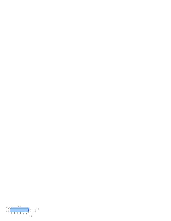
Figure 1: Plane scheme of the magnetic junction. There exists a very thin spacer between the layers 1 and 2; $\mathbf{H}$ is an external magnetic field; the layer 3 is nonmagnetic.

Two switching mechanisms may be seen from the Fig. 2 (see also [5]). The first one arises due to noncollinearity of the vectors $\mathbf{M_{1}}$ and $\mathbf{M}$ and the loss of the transversal spin components during their moving in the layer 2. The lost components transfer from the mobile electrons to the lattice [8, 9], which may excite the switching. Then the electron spins become completely collinear with $\mathbf{M}$, but remain nonequilibrium ones. The second mechanism arises at this stage. Equilibrium distribution (among the spin energy subbands) should be restored and processes go, which may lead to $\mathbf{M}$ instability and switching [11, 12].

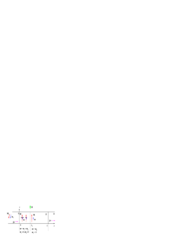
Figure 2: Scheme of processes in the layers of the junction.

3 Equations

We intentionally exclude from consideration some zone between the layers 1 and 2 where a quantum nonuniform problem should be solved to describe the conduction electrons moving between the layers. Instead, we tried to derive some flux boundary conditions which allow considering the junction processes without the detail inside the zone (all the theory was presented in Refs. [2, 3, 4])). The approaches of some other authors are presented in Refs. [8, 13, 14].

The standard sd Hamiltonian is

$$U_{sd}=-\alpha_{1}\int_{-L}^{0}\mathbf{m}_{1}(x^{\prime})\mathbf{M}_{1}\,dx^{\prime}-\alpha\int_{0}^{L}\mathbf{m}(x^{\prime})\mathbf{M}(x^{\prime})\,dx^{\prime},$$ (1)

where $\alpha\sim\alpha_{1}\sim 10^{-4}$ is the dimensionless sd exchange parameter, $L_{1}\gg L$. The dynamics may be described by the following equations:

1) the continuity equation for mobile electrons

$$\frac{\partial\mathbf{m}}{\partial t}+\frac{\partial\mathbf{J}}{\partial x}+\gamma\alpha[\mathbf{m}\times\mathbf{M}]+\frac{\mathbf{m}-\bar{\mathbf{m}}}{\tau}=0,$$ (2)

where the spin flux density for mobile electrons $\mathbf{J}$ is

$$\mathbf{J}=\frac{\mu_{B}}{e}(j_{\uparrow}-j_{\downarrow})\hat{\mathbf{M}},$$ (3)

$j_{\uparrow}$ and $j_{\downarrow}$ being the partial currents, $\hat{\mathbf{M}}=\mathbf{M}/|\mathbf{M}|$ is the unit vector, $\tau$ is the spin relaxation time, $\mu_{B}$ is the Bohr magneton, $\gamma$ is the gyromagnetic ratio, $\bar{\mathbf{m}}$ is the equilibrium value;

2) the Landau–Lifshitz–Gilbert equation for $\hat{\mathbf{M}}$

$$\frac{\partial\hat{\mathbf{M}}}{\partial t}+\gamma\left[\hat{\mathbf{M}}\times\mathbf{H}_{\rm eff}\right]-\kappa\left[\hat{\mathbf{M}}\times\frac{\partial\hat{\mathbf{M}}}{\partial t}\right]=0,$$ (4)

where $\kappa$ is the Gilbert dissipation constant (typically $\kappa\sim 3\times 10^{-2}$). Effective field in Eq. (4) is

$$\mathbf{H}_{\rm eff}=\mathbf{H}+\mathbf{H}_{a}+\mathbf{H}_{d}+\mathbf{H}_{sd}+A\frac{\partial^{2}\mathbf{M}}{\partial x^{2}},$$ (5)

where $\mathbf{H}$ is the external magnetic field, $\mathbf{H}_{a}$ is the anisotropy field, $\mathbf{H}_{d}$ is the demagnetization field and $\mathbf{H}_{sd}$ is the sd exchange field. Here all the fields are defined by external conditions, except $\mathbf{H}_{sd}\equiv-\displaystyle\frac{\delta U}{\delta\mathbf{M}}$ which is a functional derivative and should be calculated from Eq. (1). We suppose very small spin relaxation time $\tau\sim 3\times 10^{-13}$ s, so that we have $\omega\tau\ll 1$ condition for the characteristic precession frequency $\omega$. Along with it, specific exchange frequency $\gamma\alpha M$ is large enough, namely, $\omega_{sd}\sim 10^{14}$ s^-1, and therefore $\omega_{sd}\tau\sim 10^{2}\gg 1$ . Based on the assumptions mentioned, we may solve Eq. (2) and substitute the solution into Eq. (1). It was exactly performed in Refs. [3, 4, 5] with the result for the nonequilibrium part of the exchange field $\mathbf{H}_{sd}$

$$\Delta\mathbf{H}_{sd}=h_{sd}\hat{\mathbf{M}}_{1}l\delta(x-0),$$ (6)

where field $h_{sd}$ is a function of the conduction electron parameters depending on the current direction (forward or backward), $l$ is the electron spin diffusion length in layer 2, and the $\delta$-function shows the field (6) is localized near the $x=0$ boundary of the layer (see the derivation in Refs. [3, 4, 5]). Thus, we present the form of equation (6) and now it is necessary to formulate the boundary conditions to solve the problem.

We formulate further the conditions of magnetic flux continuity following the results of Refs. [3, 4, 5].

The following magnetization flux densities exist in our problem [4]:

1) Free electron spin current density $\mathbf{J}$ (see (3)). It is a longitudinal flux because $\mathbf{J}\sim\hat{\mathbf{M}}$.

2) Lattice magnetization flux density $\mathbf{J}_{M}(x)=\gamma AM\left[\hat{\mathbf{M}}\times\displaystyle\frac{\partial\hat{\mathbf{M}}}{\partial x}\right]$, which is, obviously, transversal.

3) Sd exchange flux density $\mathbf{J}_{sd}(x)=\gamma h_{sd}l\left[\hat{\mathbf{M}}(0)\times\hat{\mathbf{M}}_{1}\right]\theta(x-0)$, which is transversal, $\theta(x)=1,\,x>0$ and $\theta(x)=0,\,x<0$. The general continuity condition will be

$$\mathbf{J}(+0)-\mathbf{J}(-0)+\mathbf{J}_{M}(+0)-\mathbf{J}_{M}(-0)+\mathbf{J}_{sd}(+0)-\mathbf{J}_{sd}(-0)=0.$$ (7)

The situation may be simplified for pinned layer 1 when $\mathbf{J}_{M}(-0)=\mathbf{J}_{sd}(-0)=0$ . Moreover, let us consider separately the projections for the forward and backward currents [4, 5]. Then we have for the forward current ($j/e>0$)

$$\left[\hat{\mathbf{M}}(+0)\times\left[\mathbf{J}(-0)\times\hat{\mathbf{M}}(+0)\right]\right]=\mathbf{J}_{M}(+0)+\mathbf{J}_{sd}(+0),$$ (8)

and for the backward current ($j/e<0$)

$$\left[\hat{\mathbf{M}}_{1}\times\left[\mathbf{J}(+0)\times\hat{\mathbf{M}}_{1}\right]\right]=-\mathbf{J}_{M}(+0)-\mathbf{J}_{sd}(+0).$$ (9)

In the other boundary of layer 2, that is at $x=L$, we have

$$\mathbf{J}_{M}(L-0)=0.$$ (10)

4 Instability thresholds

We solve now Eqs. (2) and (4) with boundary conditions (8)–(10). Initial magnetization is taken as $\hat{M}_{z}=\pm 1$, that is directed along $z$ axis. We search the small harmonic fluctuations $\Delta M_{x},\,\Delta M_{y}\sim\exp(-i\omega t)$ and find dispersion relations (see [3, 4, 5]). Then we obtain the following estimation of the instability threshold currents. Threshold current density $j_{\rm th}$ for the transversal channel is

$$\left|\frac{j_{\rm th}}{e}\right|_{k}=\frac{2\pi\gamma M^{2}l\lambda\kappa}{\mu_{B}Q_{1}}\left(1+\frac{1}{\nu^{\ast}}\right),$$ (11)

where $\lambda=L/l$, $Q_{1}$ is the current polarization degree in layer 1, $\nu^{\ast}=Z_{1}/Z_{3}+\lambda Z_{1}/Z_{2}$, $Z_{i}\,(i=1,\,2,\,3)$ is the spin resistance (see [5]). Estimations using Eq. (11) typically give $j_{\rm th}\sim 6\times 10^{7}\times\left(1+\displaystyle\frac{1}{\nu^{\ast}}\right)$ A/cm².

Threshold current density for the longitudinal channel is

$$\left|\frac{j_{\rm th}}{e}\right|_{p}=\frac{H_{a}l}{\mu_{B}\alpha\tau Q_{1}}\left(\lambda+\frac{Z_{2}}{Z_{3}}\right)\left(1+\frac{H\bar{\hat{M}}_{z}}{H_{a}}\right),$$ (12)

where we may substitute the typical values $H_{a}\approx 100$ Oe, $\lambda\approx 0.1\gg Z_{2}/Z_{3}$, $l\sim 10^{-6}$ cm. Then at $H=0$ we obtain the threshold $j_{\rm th}\sim 2\times 10^{5}$ A/cm² which is three orders of magnitude low than for transversal channel. Further radical reduction of the threshold may be achieved in a magnetic field $H\bar{\hat{M}}_{z}\to-H_{a}+0$. The cause of the reduction is the proximity to the reorientation phase transition in the field $H$.

5 Rod-to-film cylindrical structure

Up to now, we considered the simplest planar ferromagnetic structures. However, to obtain the highest spin injection level we should check other configurations also. Further we will focus our attention on a cylindrical structure of the rod-to-film type, the scheme of which is shown in Fig. 3. This scheme was proposed in Ref. [15]. The thickness $h$ of the film 1 is small in comparison with the radius $R$ of the rod 3. Due to continuity of the current we may get $R/2h\sim 500$ times enhancement of the current density near the edge of the rod when the current flows from the rod to the film. Then the current density may reach $10^{9}$ A/cm² or even more. It is, apparently, enough to have very high spin injection level and the inversion of spin population. The possibility of such an inversion was discussed in a number of papers [16, 17, 18, 19]. We consider below some calculations and experimental results about spin-injection and THz luminescence in the structures.

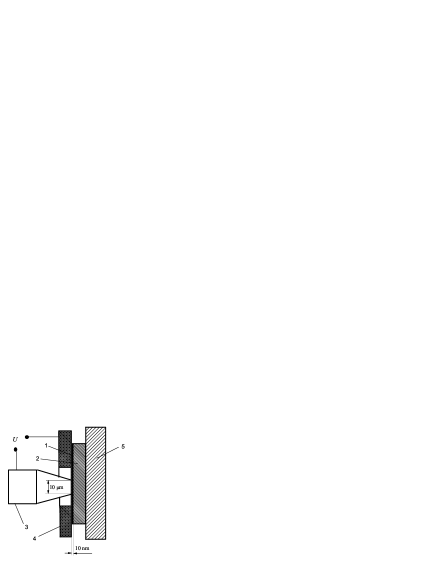
Figure 3: Structure scheme: 1–ferromagnetic film, 2–substrate, 3–ferromagnetic rod, 4– nonmagnetic conductor, 5–fluoroplastic plate, $U$–voltage.

The distribution of electron spins in the structure under electron current flowing in the rod $\to$ film direction is calculated by means of continuity equation (see [15])

$$\nabla^{2}P-\frac{(\mathbf{j}\nabla)P}{j_{D}l}-\frac{P-\bar{P}}{l^{2}}=0,$$ (13)

where $P=(n_{\uparrow}-n_{\downarrow})/n$ is the degree of spin polarization and $n_{\uparrow},\,n_{\downarrow}$ are the populations of the lower and upper spin energy subbands, $n=n_{\uparrow}+n_{\downarrow}$, $\bar{P}$ is the equilibrium polarization, $j_{D}=enl/\tau$ is a characteristic current density.

We solve Eq. (13) analytically in cylindrical coordinates using the conditions of spin flux continuity at the layer boundaries. The polarization tends to its equilibrium value $\bar{P}$, when we are moving apart from the rod edge.

The calculated $P(r)/\bar{P}$ distribution is shown in Fig. 4. Curves 1–4 correspond to rising of the spin injection level $Q_{1}/\bar{P}$: 0(1), 1(2), 2(3), 5(4). We see an inversion of spin polarization, $P(R)<0$ appears for large enough value of $Q_{1}/\bar{P}$.

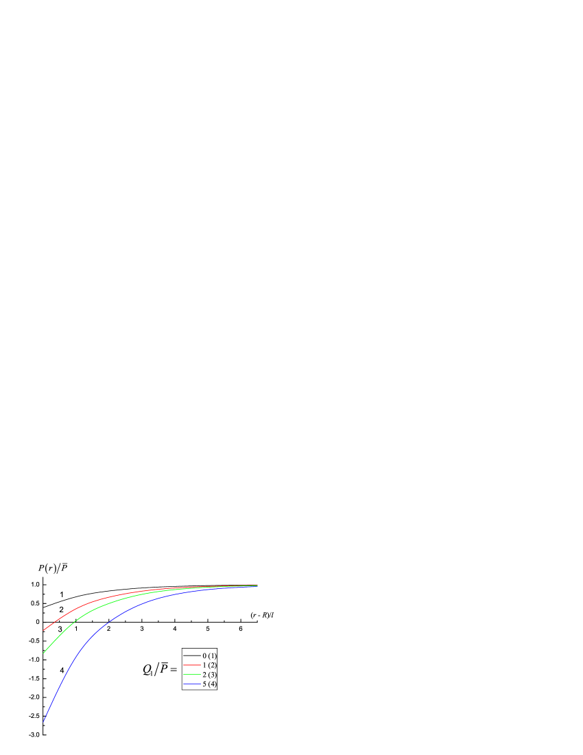
Figure 4: The calculated $P(r)/\bar{P}$ distribution is shown in the figure. The following parameters are taken: $R/l=20,\,j(R)/j_{D}=1$ and various values of $Q_{1}/\bar{P}$ ratio. We see an inversion of spin polarization, $P(r)<0$, appears for large enough value of $Q_{1}/\bar{P}$.

The calculated dependence of the relative spin polarization $P(R)/\bar{P}$ on the dimensionless current density $j(R)/j_{D}$ is shown in Fig. 5. As it is seen, the inversion of spin population ($P(R)<0$) appears also. However, for a nonmagnetic rod (curve 1, $Q_{1}/\bar{P}=0$) the inversion is absent. It means the inversion is the consequence of spin injection by the current. The negative polarization rises in magnitude with current growing, that is, with the injection level.

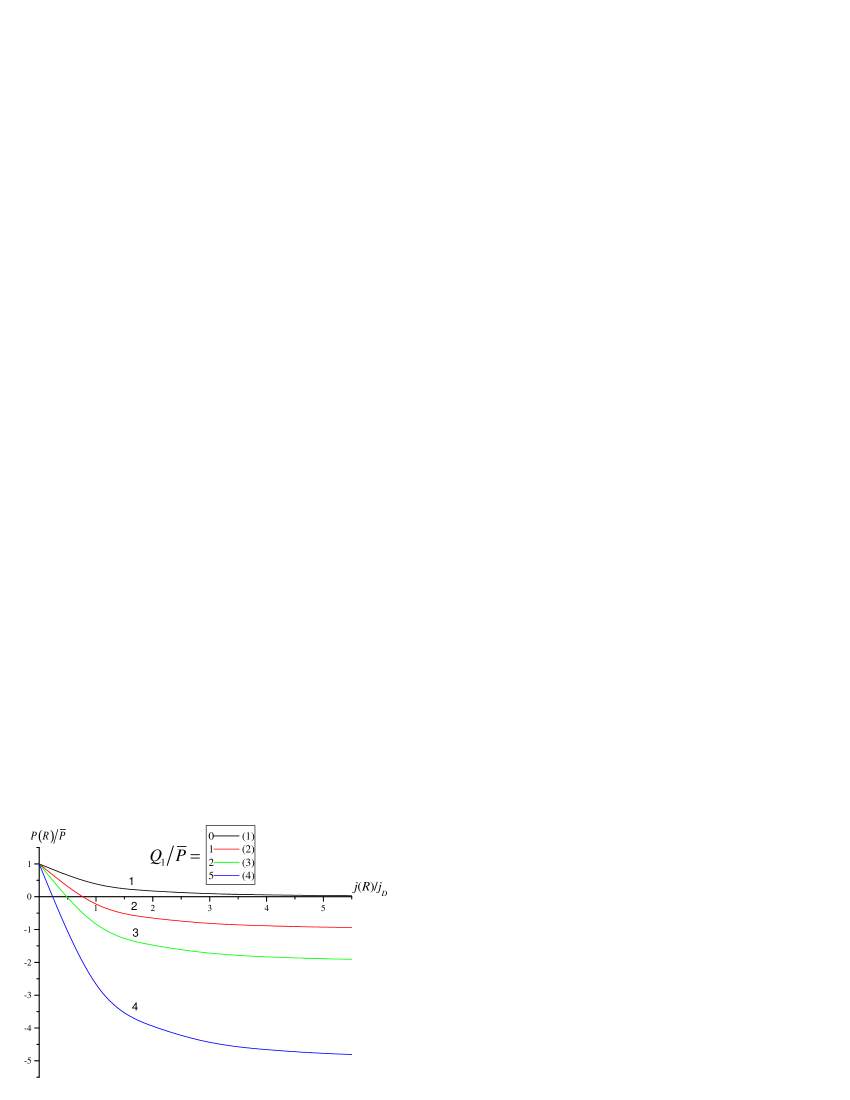
Figure 5: Spin polarization at the boundary between the rod and the film as a function of the (dimensionless) current density $j(R)/j_{D}$ at $R/l=20$ and various values of $Q_{1}/\bar{P}$ ratio.

6 Experimental observation of spin-injection luminescence

We measured the luminescence of the experimental structure (Fig. 3) by means of a Golay cell and the metallic filter to cut off frequencies below approximately 1 THz.

Measurements of luminescence intensity were carried out with the pulse current flowing in forward and backward directions. Pulses may be of different pulse period to pulse duration ratios (PPPDR) to have small and variable heating.

The results are presenting in Figs. 6 and 7. We see the measured intensity depends on the current direction. These observations cannot be explained by any thermomagnetic effects, such as Peltier or Ettingshausen effects [20]. For metals, the latter effects may be estimated as a fraction of a degree, while we have heating up to 10$\div$15 degrees. Moreover, the discussed dependence on current direction disappeared immediately after we replaced the steel rod by the nonmagnetic copper one. We conclude therefore, the direction of the current flowing influences due to magnetic properties of the rod and represents non-thermal action of the current.

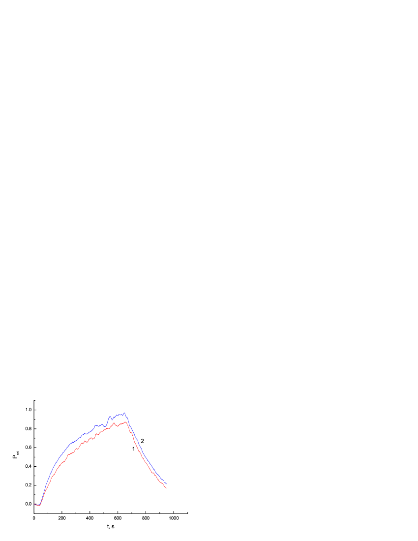
Figure 6: Measured intensity $I$ of the structure radiation intensity as a function of time for the forward (1) and backward (2) current directions, PPPDR being 5. Initially $I$ rises with time $t$ due to the current heating and spin injection. After the current is switched off, the radiation drops.

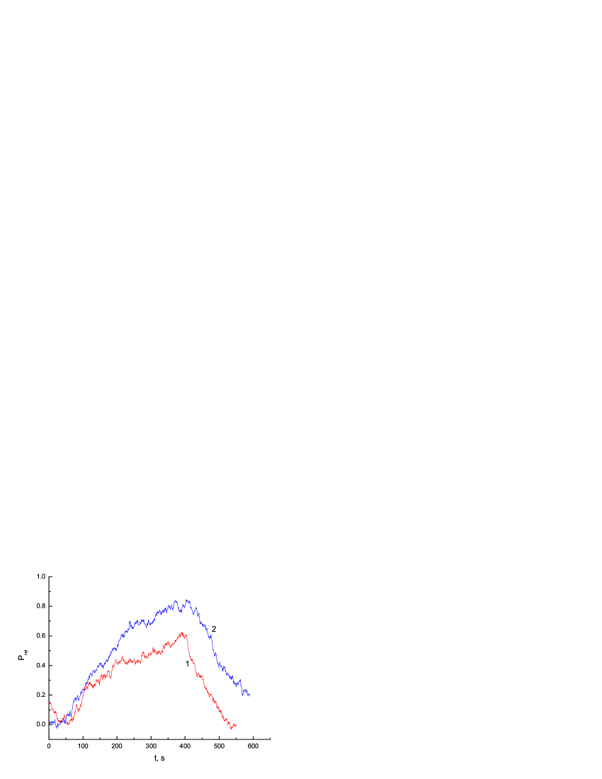
Figure 7: Measured intensity $I$ for the forward (1) and backward (2) current directions, PPPDR being 20. Thermal effect is greatly suppressed, but the difference between forward and backward current effects increases.

Based on the observations, we suggested the main role of magnetic properties of the rod and non-thermal action of the current. The luminescence really contains thermal and non-thermal contributions. However, the thermal contribution decreases with PPPDR increasing, while the non-thermal contribution remains stable. That is the main cause of the splitting curves 1, 2 in Figs. 6 and 7.

We may use now the results of spin-injection calculations derived recently in [15]. According to Eq. (20) from the Ref. [15], we represent the highest (in magnitude) negative value of the nonequilibrium spin polarization achieved in film near the boundary of the rod in the form

$$|\Delta P|=\left|\left[Q_{1}\left(\hat{\mathbf{M}}_{1}\cdot\hat{\mathbf{M}}(R)\right)-\bar{P}\right]\frac{j(R)}{j_{D}}\frac{K_{\nu}(R/l)}{K_{\nu+1}(R/l)}\right|,$$ (14)

where $K_{\nu}$ is the modified Bessel function of the second kind with index

$$\nu=\frac{1}{2}\frac{R}{l}\frac{j(R)}{j_{D}}.$$ (15)

The most significant consequence of the formulae (14) and (15) is the fact that the nonequilibrium polarization $\Delta P$ depends on the current both directly and via the index $\nu$, being nonsymmetrical with respect to changing the current sign, $j\to-j$. Therefore the spin injection contributes to $\Delta P$, and the contribution is different for forward and backward directions of the current. The absolute difference between the contributions, according to the formulae, have no small parameters and, in principle, may be sufficient to explain the splitting 1, 2 curves in Figs. 6 and 7.

7 Summary

The conduction electrons that participate in polarized current (s electrons) interact with the lattice magnetization (d electrons) in a ferromagnetic junction via two channels: (i) via the transfer of the transverse spins (perpendicular to the lattice magnetization) to the lattice, and (ii) via the transfer of the longitudinal spins parallel to the magnetization to the spin energy subbands. The latter can be considered as a change in the population of spin energy subbands, i.e., the injection of nonequilibrium spins. This injection leads to the creation of a nonequilibrium sd exchange effective field, which, in turn, affects the dynamics of the system, in particular: 1) the lowering of magnetic exchange instability threshold, and 2) creation of the inversion subband population and negative effective spin temperature.

We should provide some specific relations between the spin resistances of the layers $Z_{i}$, where $i=1,\,2,\,3$ labels the layers. In particular, $Z_{2}\ll Z_{1},\,Z_{3}$ condition leads to reduction in the threshold. The estimates for some typical samples show the threshold can be lowered by orders of magnitude, for example, from $\sim 6\times 10^{7}$ to $2\times 10^{5}$ A/cm². The minimum thresholds always correspond to the predominance of the spin-injection channel of the sd exchange interaction.

An external magnetic field $H$ which is near the critical value $H_{c}$ for a reorientation phase transition ($H=H_{c}-0$) can lead also to radical lowering of the exchange current threshold. The external magnetic field, being near the phase transition point and acting together with the exchange field, helps the exchange switching. We investigated also the junctions having variable lateral dimensions of the layers, the so called rod-to-film structures. Very high current density and spin-injection level may be achieved in the structures. Two interesting facts have been observed in our measurements: 1) the presence of non-thermal contributions to THz luminescence from the system in study, and 2) the difference between the radiation intensities under the forward and backward current directions. As it was shown (see Eqs. (14) and (15)), the spin injection in the junction depends substantially on the current direction. Therefore, the facts mentioned may be due to the radiation created by the nonequilibrium spins injected near the rod.

References

- [1] S.V. Vonsovskii, Magnetism (Wiley, New-York 1974).
- [2] Yu.V. Gulyaev, P.E. Zilberman, E.M. Epshtein, and R.J. Elliott, J. Exp. Theor. Phys. 100, 1005 (2005).
- [3] E.M. Epshtein, Yu.V. Gulyaev, and P.E. Zilberman, arXiv:cond-mat/0606102v2.
- [4] Yu.V. Gulyaev, P.E. Zilberman, A.I. Panas, and E.M. Epshtein, J. Exp. Theor. Phys. 107, 1027 (2008).
- [5] Yu.V. Gulyaev, P.E. Zilberman, A.I. Panas, and E.M. Epshtein, Physics–Uspekhi 52, 335 (2009).
- [6] A. Fert, Rev. Mod. Phys. 80, 1517 (2008).
- [7] P.A. Grünberg, Rev. Mod. Phys. 80, 1531 (2008).
- [8] J.C. Slonczewski, J. Magn. Magn. Mater. 159, L1 (1996).
- [9] L. Berger, Phys. Rev. B 54, 9353 (1996).
- [10] E.B. Myers, D.C. Ralph, J.A. Katine, R.N. Louie, and R.A. Buhrman, Science 285, 867 (1999).
- [11] C. Heide, P.E. Zilberman, and R.J. Elliott, Phys. Rev. B 63, 064424 (2001).
- [12] Yu.V. Gulyaev, P.E. Zilberman, E.M. Epshtein, and R.J. Elliott, JETP Lett. 76, 155 (2002).
- [13] M.D. Stiles and A. Zangwill, Phys. Rev. B 66, 014407 (2002).
- [14] M.D. Stiles, J. Xiao, and A. Zangwill, Phys. Rev. B 69, 054408 (2004).
- [15] Yu.V. Gulyaev, P.E. Zilberman, A.I. Panas, S.G. Chigarev, and E.M. Epshtein, J. Commun. Technol. Electron. 55, 668 (2010).
- [16] V.V. Osipov and N.A. Viglin, J. Commun. Technol. Electron. 48, 548 (2003).
- [17] A.M. Kadigrobov, Z. Ivanov, T. Claeson, R.I. Shekhter, and M. Jonson, Europhys. Lett. 67, 948 (2004).
- [18] Yu.V. Gulyaev, P.E. Zilberman, A.I. Krikunov, A.I. Panas, and E.M. Epshtein, JETP Lett. 85, 160 (2007).
- [19] N.A. Viglin, V.V. Ustinov, and V.V. Osipov, JETP Lett. 86, 193 (2007).
- [20] F.J. Blatt: Physics of Electronic Conduction in Solids (McGraw-Hill Book Company, 1968).