On correlations in high-energy hadronic processes and the CMS ridge:
A manifestation of quantum entanglement?

Abstract

We discuss the possibility of quantum entanglement for pairs of charged particles produced in high-energy $pp$-collisions at the LHC. Using a framework of interacting Wilson lines, we calculate 2-D and 1-D two-particle angular correlation functions in terms of the differences of the pseudorapidities and azimuthal angles of the produced particles. The calculated near-side angular correlation shows a localized maximum around $\Delta\phi\approx 0$, though it is less pronounced compared to the peak observed by the CMS Collaboration. We argue that this soft correlation is universal and insensitive to the specific properties of the matter (quark-gluon plasma, QCD vacuum, etc.) used to describe hadronic states—though such properties can be included to further improve the results.

I Introduction

The CMS collaboration at the Large Hadron Collider (LHC) of CERN observed last year CMS_2010_ridge significant two-particle angular correlations of charged particles, produced in proton-proton ($pp$) collisions at a center-of-mass energy $\sqrt{s}=7\ {\rm GeV}$. These correlations are of long-range nature in the pseudorapidity difference $2.0<|\Delta\eta|<4.8$ and appear on a three-dimensional (3-D) plot of the $\Delta\eta-\Delta\phi$ correlation function as a clearly seen ridge-like structure on the near-side $\Delta\phi\approx 0$. Here $\Delta\eta=\eta_{1}-\eta_{2}$ is the difference in the pseudorapidity $\eta=-\ln[\tan(\theta/2)]$ between the two produced particles, where $\theta$ is the polar angle relative to the beam axis, and $\Delta\phi=\phi_{1}-\phi_{2}$ is the difference in their azimuthal angle. The ridge becomes most pronounced for intermediate transverse momenta $1\ {\rm GeV}<p_{\perp}<3\ {\rm GeV}$ and in events with an average charged-particle multiplicity of at least $N\approx 90$, whereas simulations using Monte Carlo (MC) models do not predict such an effect—independent of multiplicity and transverse momentum. No evidence for such near-side long-range correlations has been found in the $pp$ or $p\bar{p}$ data before, though the novel ridge structure is reminiscent of correlations observed in nuclear collisions at the Relativistic Heavy Ion Collider (RHIC) at Brookhaven National Laboratory PHOBOS07 ; PHOBOS10 ; STAR10 . However, these correlations were assumed to arise from interactions of the produced particles with the medium and from collective effects in the initial-state interactions of the nuclei.

Adopting the notations of Corr_Def ; PHOBOS07 , the two-particle correlation function can be defined as follows:

$$R(\eta_{1},\phi_{1},\eta_{2},\phi_{2})=\Bigg{\langle}\!\!(\langle N\rangle-1)\!\left(\frac{\rho_{II}(\eta_{1},\phi_{1},\eta_{2},\phi_{2})}{\rho_{I}(\eta_{1},\phi_{1})\rho_{I}(\eta_{2},\phi_{2})}-1\right)\!\!\!\Bigg{\rangle}\ ,$$ (1)

where $\rho_{I}(\eta,\phi)$ and $\rho_{II}(\eta_{1},\phi_{1},\eta_{2},\phi_{2})$ denote single and double particle distributions in the final state, respectively Corr_Def . In what follows, we will express the correlation function in terms of parton distributions which differ, in general, from those of real particles (hadrons). This approximation is justified because the correlations under consideration emerge long before the hadronization starts, so that the process can be adequately described in terms of partons. In the context of the CMS experiment, $\rho_{II}(\eta_{1},\phi_{1},\eta_{2},\phi_{2})$ resembles $S_{N}$, i.e., the signal distribution, whereas the product of the single parton distributions plays the role of the random background distribution $B_{N}$—cf. Eqs. (4.2) and (4.3) in CMS_2010_ridge . Moreover, $\langle N\rangle$ is the number of tracks per event averaged over the multiplicity bin and $R(\Delta\eta,\Delta\phi)$ is determined by averaging over multiplicity bins and over $(\eta_{1}+\eta_{2})$ and $(\phi_{1}+\phi_{2})$—see Corr_Def . These quantities will be specified and discussed in detail within our theoretical framework later.

A wide pseudorapidity range of correlated charged-particle pairs indicates that the source of the correlation has to be primordial, in the sense that it emerges coincidentally with the particle production, but before hadronization occurs (see, e.g., CGC_2009 ; CGC_2010 ). Theoretical attempts to dig out the physical origin of the ridge structure in the high-multiplicity $pp$ data observed by CMS mainly concentrate on the properties of a particular state of matter—the Color Glass Condensate (CGC)—that was created during the high-energy collision (see, for instance, Refs. Shuryak ; CGC_2010 ; IHEP10 ). Other authors claim that the observed ridge may be the manifestation of an azimuthal quadrupole TK10 , or the result of reflective scattering effects in multiparticle production processes IHEP11 . Further references concerning the ridge formation mechanisms can be found in CMS_TH_new , where the CMS Collaboration have updated their analysis to include the full 2010 statistics.

We are going to approach the emergence of the ridge phenomenon from another side which has echoes of our previous works on the gauge invariance of transverse-momentum-dependent (TMD) parton distribution functions (PDF)s (see CS_all ; CKS_2010 , and SC09 for reviews). To be precise, we intend to discuss effects ensuing from nonlocal path-dependent interactions—the latter naturally arising in the gauge-invariant description of high-energy processes with charged particles in terms of Mandelstam fields Man62 . We will argue in what follows that the inclusion of semi-infinite gauge links (Wilson lines) gives rise to a phase that in some sense is akin to the intrinsic Coulomb phase found by Jakob and Stefanis (JS) JS91 in QED by employing Mandelstam’s gauge-invariant path-dependent formalism. The origin of the intrinsic Coulomb phase can be considered as a residual effect of the primordial separation of the particle from its oppositely charged counterpart and has no bearing on external charge distributions.

Adopting this viewpoint, we will work out a scheme which will enable us to calculate the leading-order contribution to the two-dimensional (2-D) $\Delta\eta-\Delta\phi$ correlation function of interacting Wilson lines. The justification for such a treatment is provided by the fact that Wilson lines can be recast in the form of particle worldlines in the context of first-quantized theories Pol79 . Therefore, this scheme lends itself to the actual experimental situation in which charged particles are emitted in the $pp$ collisions at a very high center of mass energy $\sqrt{s}$ of 0.9, 2.36, and 7 TeV, forming highly collimated jets before they finally hadronize. The key idea here is that as the number of such particle tracks increases, several pairs of them are created in unison (with regard to their separation in $\Delta\eta$ and $\Delta\phi$), so that the quantum mechanism of entanglement applies. Note in this context that it is not necessary to consider these pairs as being formed by particles with opposite polarities, as discussed by JS in the special case of the QED intrinsic Coulomb phase. In fact, the CMS data analysis CMS_2010_ridge has shown that the results for like-sign and unlike-sign pairs agree with each other within uncertainties. Also our calculation does not depend on the sign of the correlated pairs. As we will see below, the obtained result shows a clear and significant ridge-like structure in the plane of the differences in pseudorapidity and azimuthal angle between the interacting Wilson lines, which occurs around $\Delta\phi\approx 0$ and extends over a wide range of $\Delta\eta$, albeit the near-side peak is less prominent compared to that observed by CMS. The rest of the paper is organized as follows. In the next section, we recall the main features of the intrinsic Coulomb phase in QED in order to sketch the main idea underlying the present application. Our theoretical approach to understand the ridge structure and the comparison with the experimental findings of the CMS Collaboration are presented in Sec. III. In Sec. IV, we give a summary of our results and discuss them further. Finally, in Sec. V we draw our conclusions.

II Intrinsic Coulomb phase in QED

It is worth indulging in a quick detour into the nature of the “intrinsic” Coulomb phase JS91 which is an extreme case of quantum entanglement because it persists even for infinitely separated particles.

Within the JS path-dependent approach, charged fields are always accompanied by a soft-photon cloud in terms of a non-integrable phase factor which contains a timelike straight line stretching to infinity. In the presence of other charges, the charged field acquires a relativistic Coulomb phase, in accordance with the results obtained earlier by Kulish and Faddeev KF70 , and independently by Zwanziger Zwa_all . But, it also yields an additional phase that does not depend on external charge distributions and remains different from zero, even if the conventional Coulomb phase vanishes—hence, the name “intrinsic”. The origin of this phase was ascribed by JS to the asymptotic interaction of the charged particle with its oppositely charged counterpart that was removed “behind the moon” instantaneously after their common primordial creation. The mechanism of the particle creation, as well as that of their separation, is irrelevant for these considerations. What counts is that they have been created in common, i.e., entangled. Speaking in more technical terms, the intrinsic Coulomb phase is acquired during the parallel transport of the charged field along a timelike straight line from infinity to the point of interaction with the photon field and is absent in the local approach, i.e., for charged fields joined by a (gauge) connector (see, e.g., Ste83 for more details). It is different from zero only for a Mandelstam field, which has its own gauge contour attached to it, and keeps track of its full history since its primordial entangled creation with its antiparticle. Let us also mention that the existence of a balancing charge “behind the moon” was postulated before by several authors—see JS91 for related references—in an attempt to restore the Lorentz covariance of the charged sector of QED. Therefore, the discussed mechanism of phase entanglement originates from quite general features of gauge field theory and is insensitive to the specific properties of the particular process under consideration. We want to make it clear at this point that we are not advocating a violation of the principle of locality: nothing can cross a void linking cause to effect—except a phase.

The simplest non-Abelian generalization of the intrinsic Coulomb phase for the quark fields reads (in leading order of the strong coupling constant $\alpha_{s}$ indicated by the superscript $(1)$)

$$\Phi^{(1)}(\Gamma)=\ -4\pi\int_{{\Gamma}}\!dx_{\mu}\int d^{4}zD_{ab}^{\mu\nu}(x-z)t^{a}j_{\nu}^{b}(z)\ ,$$ (2)

where $D_{ab}^{\mu\nu}$ is the (free) gluon propagator, and the current $j_{\nu}^{b}(z)=t^{b}v_{\nu}\int_{\Gamma}d\tau\delta^{(4)}(z-v\tau)$ describes the residual effects of the oppositely charged counterpart in a semiclassical approximation. The integration path $\Gamma$ is the contour defined by the kinematics of the process and can have a complicated structure venturing off-the-light-cone in the transverse direction CS_all ; CS10 . Note that the phase (2) can be considered as the leading non-trivial term of the expansion of a non-Abelian path-ordered exponential KR87 in the ground state (abbreviated by GS), i.e.,

$$\Phi(\Gamma)=\exp\left[\sum_{n=1}^{\infty}\alpha_{s}^{n}\Phi^{(n)}(\Gamma)\right]=\left\langle{\rm GS}\left|{\cal P}\exp\Big{[}ig\int_{\Gamma}\!d\zeta^{\mu}\ t^{a}A^{a}_{\mu}(\zeta)\Big{]}\right|{\rm GS}\right\rangle\ .$$ (3)

As we shall show shortly, the path dependence of the phase factor in (3) becomes crucial in the application of the Mandelstam formalism in studying semi-inclusive processes in QCD.

III CMS ridge—theoretical considerations

The appearance of long-range correlations in nuclear collisions at RHIC RHIC05-10 and (very recently) in $pp$-collisions at the LHC CMS_2010_ridge has been studied within the color-glass-condensate approach in CGC_2009 ; CGC_2010 (see also the more recent papers Shuryak ; IHEP10 ). In our study we refrain from making any assumptions about the structure of the quark-gluon (QG) matter just-before/during/just-after the proton-proton collisions, and appeal instead to a field theoretic description of the particle tracks in terms of path-dependent exponentials along the lines exposed above. Nevertheless, the properties of the QG-matter can be taken into account within our approach by means of a specification of the ground state entering the evaluation of matrix elements with Wilson-line exponentials.

To make qualitative estimates, we will now expose our working method to treat the semi-inclusive process of the two-particle production in the proton-proton collision in more mathematical terms and start by writing

$$h(p_{1})+h(p_{2})\ \to\ y(p_{3})+y(p_{4})+{\cal X}\ .$$ (4)

In what follows, we try to understand this process from the point of view of the QCD factorized cross-section, our goal being to figure out what part(s) of this factorized expression is (are) responsible for the above-mentioned ridge-like structure. Keep in mind that the observed correlations have to be nonlocal and primordial so that our task consists in identifying which part in the factorized expression can serve as the root cause of such a phenomenon. The (symbolic) factorization formula reads

$${d\sigma}\sim H\otimes\tilde{\cal F}_{\rm D_{1}}\otimes\tilde{\cal F}_{\rm D_{2}}\otimes\tilde{\cal F}_{\rm F_{1}}\otimes\tilde{\cal F}_{\rm F_{1}}+{\rm power\ suppressed\ terms}\ ,$$ (5)

while a detailed discussion of this expression and references can be found, for instance, in Refs. S79 ; Col03 ; JMY04 ; BR05 ; CRS07 . Problems related to the factorization and universality of TMD PDFs, etc., are considered in Refs. BM07 ; CQ07 ; RM2010 . Note that these issues are not crucial for our discussion. We will demonstrate below that the correlations under consideration can be described by the interaction of Wilson lines without explicit reference to the factorization formula. The acronyms used in the above equation and below have the following meaning: PFF—parton fragmentation function; DF—distribution function; FF—fragmentation function, so that the subscripts ${\rm D,F}$ are labels for ‘distribution’ and ‘fragmentation’, respectively. Note that the right place to take into account TMD PDFs is the moderate $p_{\perp}$ region $1\ {\rm GeV/c}<p_{\perp}<3\ {\rm GeV/c}$, where the intrinsic transverse momenta of the partons become relevant, while at larger $p_{\perp}$ the transverse momentum is mostly generated by perturbative hard-gluon exchanges.

Given these circumstances, one has to dig out the origin of the long-range primordial correlations employing the above factorization theorem. We will argue that the observed two-particle correlation has its origin in the soft factors which are indispensable for the renormalization of the TMD PDFs CS_all . Each DF (or FF) has its own soft part, so that the above factorization becomes

$${d\sigma}\sim H\otimes[{\cal F}_{\rm D_{1}}\cdot S_{\rm D_{1}}]\otimes[{\cal F}_{\rm D_{2}}\cdot S_{\rm D_{2}}]\otimes[{\cal F}_{\rm F_{1}}\cdot S_{\rm F_{1}}]\otimes[{\cal F}_{\rm F_{1}}\cdot S_{\rm F_{2}}]+{\rm power\ suppressed\ terms}\ .$$ (6)

The soft terms can be properly defined in terms of expectation values of Wilson-line exponentials evaluated along particular (integration) gauge contours, specified in Refs. CS_all ; CKS_2010 , which enter expressions like

$$S_{\rm\alpha}=\left\langle{\rm GS}\left|{\cal P}\exp\Big{[}ig\int_{\Gamma}\!d\zeta^{\mu}\ t^{a}A^{a}_{\mu}(\zeta)\Big{]}\right|{\rm GS}\right\rangle\ ,$$ (7)

with the subscript $\alpha$ labeling the various factors in Eq. (6). These soft factors serve to eliminate overlapping divergences originating from interrelated short and large-scale effects that cannot be cured by (dimensional) regularization when calculating correlators of contour-dependent quark and gluon operators. It can be linked to a cusp in the gauge contour at light-cone infinity and gives rise to a non-integrable phase factor CS_all .

To implement our considerations, we define the following correlation function in terms of the soft factors of the fragmentation functions (the latter describing the hadronization process), considering it as a simplified version of the true correlation function given by (1):

$$K_{\rm soft}(\eta_{1},\phi_{1};\eta_{2},\phi_{2})=\frac{S_{\alpha\beta}(\eta_{1},\phi_{1},\eta_{2},\phi_{2})}{S_{\alpha}(\eta_{1},\phi_{1})S_{\beta}(\eta_{2},\phi_{2})}-1\ .$$ (8)

Taking into account that the soft factors enter the definition of TMD fragmentation functions multiplicatively, we assume that the soft correlation function (8) can be used as a (separately calculable) correction to the full correlation function $R(\Delta\eta,\Delta\phi)$ that also includes the non-soft contributions from the TMD PFFs. Our task is, therefore, to demonstrate that the soft function (8) gives rise to the long-range rapidity contributions that cannot be obtained without soft factors. The soft factors, which describe distribution functions of particle worldlines (tracks), are defined by

$$S_{\alpha\beta}(\eta_{1},\phi_{1},\eta_{2},\phi_{2})=\left\langle{\rm GS}\left|{\cal P}\exp\left[ig\int_{\Gamma_{\alpha{\phantom{\beta}}}}\!d\zeta^{\mu}\ t^{a}A^{a}_{\mu}(\zeta)\right]\cdot{\cal P}\exp\left[ig\int_{\Gamma_{\beta}}\!d\zeta^{\mu}\ t^{a}A^{a}_{\mu}(\zeta)\right]\right|{\rm GS}\right\rangle$$ (9)

and

$$S_{\alpha}(\eta_{1},\phi_{1})S_{\beta}(\eta_{2},\phi_{2})=\left\langle{\rm GS}\left|{\cal P}\exp\left[ig\int_{\Gamma_{\alpha{\phantom{\beta}}}}\!d\zeta^{\mu}t^{a}A^{a}_{\mu}(\zeta)\right]\right|{\rm GS}\right\rangle\cdot\left\langle{\rm GS}\left|{\cal P}\exp\left[ig\int_{\Gamma_{\beta}}\!d\zeta^{\mu}t^{a}A^{a}_{\mu}(\zeta)\right]\right|{\rm GS}\right\rangle$$ (10)

and are path-dependent quantities because they depend on the gauge contours. Referring again to Eq. (6), we note that the integration contours $\Gamma_{\alpha}$ and $\Gamma_{\beta}$ are similar in structure, but they are separated from each other by the transverse distance $\mbox{\boldmath$b$}_{\perp}$ which is equal to the impact parameter of the collision, as illustrated in the left panel of Fig. 1. Hence, the two-particle correlation function of experimental tracks transforms in our scheme into the correlation function of the worldlines of auxiliary particles moving along the gauge contours entering the soft factors and can be parameterized in terms of their separation in pseudorapidity and azimuthal angle. Pictorially, this theoretical setup of Wilson (or world-) lines looks like a sheaf of wheat within a small conus of less than about $10$ degrees corresponding to a $\Delta\eta$ of 2.44. Hence, pairs of these Wilson lines will be likely produced in association and may form an entangled quantum state, giving rise to long-range $\Delta\eta,\Delta\phi$ correlations. The evaluation of the above expressions below proceeds by calculating all Feynman graphs which emerge from the perturbative expansion of the path-ordered exponentials and retaining only the leading-order terms of order $g^{2}$.

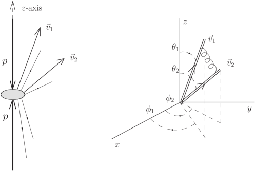
Figure 1: Left panel: Visualization of the $pp$-collision along the $z$ axis, with a multiparticle final state and two produced particles (propagating along the vectors $\vec{v}_{1}$ and $\vec{v}_{2}$) being detected and analyzed. Right panel: Schematic illustration of interacting soft factors (Wilson lines)—denoted by double lines—which enter the fragmentation functions of two particles with the momenta $p_{1}$ and $p_{2}$. The polar angles $\theta_{1,2}$ and the azimuthal angles $\phi_{1,2}$ correspond to the experimental situation in the CMS experiment, with the $z-$axis pointing along the beam direction. Only the one-gluon exchanges are shown which give rise to non-trivial angle-dependent contributions.

To start, note that the correlation function (1) depends on the Minkowski angle between the longitudinal parts of the Wilson lines, $(p_{1}^{\parallel}\cdot p_{2}^{\parallel})\sim\cosh\Delta Y$, (where $\Delta Y$ is the difference of the rapidities) and on the azimuthal angle $\Delta\phi$ between their transverse parts, i.e., $(p_{1}^{\perp}\cdot p_{2}^{\perp})\sim\cos\Delta\phi$ (see the right panel of Fig. 1 for an illustration). Thus, azimuthal correlations of the interacting Wilson lines (alias particle worldlines), entering the soft factors, can be linked to their transverse-momentum dependence, thus facilitating the computation. Then, in leading order $O(g^{2})$, the only non-trivial angular dependence stems from the correlator of two semi-infinite Wilson lines, evaluated along the rays defined by the dimensionless four-vectors $v_{1}$ and $v_{2}$. These vectors imitate the momentum vectors of the produced particles $p_{1,2}=mv_{1,2}$ with $v_{1,2}^{2}=1$. For the sake of convenience, we fix in Fig. 1 the longitudinal and the transverse axes of the mock CMS experimental setup along the directions $z$ (beam axis) and $x$, respectively.

The momentum vectors of the particles in the final state are defined as

$$p_{1,2}^{0}=m_{T}\cosh Y_{1,2},\quad p_{1,2}^{z}=m_{T}\sinh Y_{1,2},\quad p_{1,2}^{x}=p_{\perp}\cos\phi_{1,2},\quad p_{1,2}^{y}=p_{\perp}\sin\phi_{1,2}\ ,$$ (11)

where $Y_{1,2}$ are the rapidities, $\phi_{1,2}$ denote as before the azimuthal angles of the produced particles, and $m^{2}=m_{T}^{2}-p_{\perp}^{2}$. The above parametrization is more suitable for four-dimensional worldlines than that based on three-dimensional spherical coordinates with the pseudorapidity $\eta=-\ln[\tan(\theta/2)]$ and

$$p_{1,2}^{0}=E,\quad p_{1,2}^{z}=p_{\perp}\sinh\eta_{1,2},\quad p_{1,2}^{x}=p_{\perp}\cos\phi_{1,2},\quad p_{1,2}^{y}=p_{\perp}\sin\phi_{1,2}\ .$$ (12)

In the limit $p_{\perp}\gg m$, for which $\eta\to Y$, both parameterizations coincide. This approximation is natural, for instance, for pions, so that in what follows we will make use of the “worldline-friendly” parametrization (11).

Then, by definition, the leading-order non-trivial angle-dependent term of Eq. (8) reads

$$K^{(1)}(Y_{1},Y_{2},\phi_{1},\phi_{2};p_{\perp},m_{T})=\frac{[1+(ig)^{2}v_{1}^{\mu}v_{2}^{\nu}\int_{0}^{\infty}\int_{0}^{\infty}\!d\sigma_{1}d\sigma_{2}D_{\mu\nu}(z_{12})]^{-1}}{[1+(ig)^{2}v_{1}^{\mu}v_{1}^{\nu}\int\int\!d\sigma_{1}d\sigma_{2}D_{\mu\nu}(z_{1})]^{-1}[1+(ig)^{2}v_{2}^{\mu}v_{2}^{\nu}\int\int\!d\sigma_{1}d\sigma_{2}D_{\mu\nu}(z_{2})]^{-1}}-1\ ,$$ (13)

where $D_{\mu\nu}(z)$ is the free gauge-field propagator and $z_{12}^{\rho}=(v_{1}^{\rho}\sigma_{1}\pm v_{2}^{\rho}\sigma_{2}\pm b^{\rho})$, with $b_{\rho}$ being purely transverse, i.e., $b_{\rho}=(0,0,\mathbf{b}_{\perp})$, so that $z_{1,2}^{\rho}=(v_{1,2}^{\rho}\sigma_{1}\pm v_{1,2}^{\rho}\sigma_{2})$. Employing a covariant gauge, it is convenient to express the gluon propagator in the following general form (tacitly performing a dimensional regularization of the UV divergences in terms of $\omega=4-2\epsilon$ and by using the auxiliary infrared (IR) cutoff $\lambda^{2}$)

$$D_{\mu\nu}(z)=g_{\mu\nu}\partial^{2}D_{1}(z^{2})-\partial_{\mu}\partial_{\nu}D_{2}(z^{2})\ ,$$ (14)

where

$$\partial^{2}=2\omega\partial+4z^{2}\partial^{2},\ \partial_{\mu}\partial_{\nu}=2g_{\mu\nu}\partial+4z_{\mu}z_{\nu}\partial^{2},\ \partial\equiv\partial_{z^{2}}\ .$$ (15)

The above representation allows in Eq. (13) the separate calculation of the integrals over $\sigma_{1}$ and $\sigma_{2}$ by carrying out a Laplace transformation of the functions $D_{1,2}$ and their derivatives $D_{1,2}^{(k)}$:

$$D_{1,2}^{(k)}(z^{2};\epsilon,\mu^{2},\lambda^{2})=(-1)^{k}\int_{0}^{\infty}\!d\alpha\alpha^{k}{\rm e}^{-\alpha z^{2}}\ \tilde{D}_{1,2}(\alpha;\epsilon,\mu^{2},\lambda^{2})\ .$$ (16)

Hence, the angular dependence stems solely from the integral

$$\int_{0}^{\infty}\int_{0}^{\infty}\!d\sigma_{1}d\sigma_{2}{\rm e}^{-\alpha z_{\mu}z^{\mu}}=\int_{0}^{\infty}\int_{0}^{\infty}\!d\sigma_{1}d\sigma_{2}{\rm e}^{-\alpha(v_{1}\sigma_{1}-v_{2}\sigma_{2}-b)^{2}}\ .$$ (17)

In general, the scalar products $(v_{1,2}\cdot b)$ are not vanishing, so that the result of the integration in Eq. (17) is complicated. However, for our purposes it suffices to evaluate this expression using the following approximations: First, we employ the Feynman gauge and consider the gauge field as being Abelian, given that at the order $g^{2}$ of the expansion the nonlinear terms in the gluon field do not contribute. This gives

$$D_{\mu\nu}(z)=-ig_{\mu\nu}\int\!\frac{d^{4}k}{(2\pi)^{4}}\frac{{\rm e}^{-ik\cdot z}}{k^{2}-\lambda^{2}+i0}$$ (18)

with the result that in Eq. (14) $D_{2}=0$. Next, we restrict our attention to the case of collinear kinematics, i.e., when the transverse distance $\mathbf{b}_{\perp}$ equals zero, appealing to the fact that worldlines are collimated within a very narrow conus with $\Delta\eta$ values in the range $2.0<|\Delta\eta|<4.8$. In this case, the angular dependence stems only from Eq. (17), recalling that $v_{1,2}^{2}=1$, $\mathbf{b}_{\perp}=0$ and defining

$$A(Y_{1},Y_{2},\phi_{1},\phi_{2})=(v_{1}\cdot v_{2})=\frac{1}{m^{2}}\left(m_{T}^{2}\ \cosh\Delta Y-p_{\perp}^{2}\ \cos\Delta\phi\right)\ ,$$ (19)

where $\Delta\phi=\phi_{1}-\phi_{2}$, and $\Delta Y=Y_{1}-Y_{2}$.

                                          

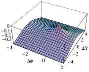
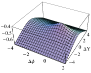
Figure 2: 2-D representation of the leading-order angular part $K^{(1)}(\Delta Y,\Delta\phi)$ of the total two-particle correlation function—given by Eq. (8)—in terms of interacting Wilson (world-) lines vs. $\Delta Y$ and $\Delta\phi$ for (from left to right) $[m_{T}=3.5,p_{\perp}=3.4],\ [m_{T}=5.0,p_{\perp}=4.9]$, and $[m_{T}=150.0,p_{\perp}=140.0]$ in units of MeV. The strong coupling constant and the UV- and IR-regulators are fixed to give $\alpha_{s}\ln\mu^{2}/\lambda^{2}=0.1$.

It is remarkable that $A$ (and, as a consequence, the whole function $K^{(1)}$) depends only on the differences of the rapidities and the azimuthal angles of the produced particles, so that we do not have to average over their sums. Hence, we have

$$A(Y_{1},Y_{2},\phi_{1},\phi_{2})=A(\Delta Y,\Delta\phi)\ ,$$

which represents a major advantage of parametrization (11). Then, we get

$$\int_{0}^{\infty}\int_{0}^{\infty}\!d\sigma_{1}d\sigma_{2}{\rm e}^{-\alpha(\sigma_{1}^{2}+\sigma_{2}^{2}\pm 2A\sigma_{1}\sigma_{2})}=\frac{\pm\pi\mp 2\arctan\sqrt{\frac{A^{2}}{1-A^{2}}}}{4\alpha\sqrt{1-A^{2}}}\ ,$$ (20)

while the UV and the IR singularities originate from the $\alpha$-integration in Eq. (16) and have been separated out from the angular part.

Therefore, performing the integrations in (13), one finds after renormalization the following expression for the angular-dependent part

$$K^{(1)}(\Delta Y,\Delta\phi;p_{\perp},m_{T})=\frac{\alpha_{s}\ C_{\rm F}}{2\pi}\ln\frac{\mu^{2}}{\lambda^{2}}\ \left[{A}\cdot\frac{\pm\pi\mp 2\arctan\sqrt{\frac{A^{2}}{1-A^{2}}}}{\sqrt{1-A^{2}}}-1\right]$$ (21)

in terms of the differences of the azimuthal angles and pseudorapidities, where $A$ is defined in Eq. (19) and $\mu$ and $\lambda$ are the UV- and IR-cutoff scales, respectively. The result for the angular part as a function of the absolute value $|\Delta Y|$ is shown graphically in Fig. 2 for different values of the parameters $m_{T}$ and $p_{\perp}$.

In order to make the ridge-like structure more visible, we first fix the value of $\Delta Y$ and display the 1-D–“slice” of the 2-D function $K(\Delta Y=4.8,\Delta\phi)$ in the left panel of Fig. 3. Following a similar procedure to that in Ref. CMS_2010_ridge , we average the two-particle azimuthal correlation function over $|\Delta Y|$ from $2.0$ to $4.8$ and plot the 1-D correlation function vs. $\Delta\phi$ in the right panel of Fig. 3. It can be compared with Fig. 8 (last 2 columns) given by the CMS Collaboration in Ref. CMS_2010_ridge .

The main observation from Fig. 2 is that the soft correlation function given by Eq. 8 reproduces the gross features of the near-side ridge structure found by the CMS Collaboration CMS_2010_ridge . In particular, it depends explicitly on the differences in rapidity and azimuthal angle between pairs of produced particles, as well as on the transverse momentum, and exhibits a localized maximum at $\Delta\phi\approx 0$ that extends to larger values of $\Delta Y$. However, it is much less pronounced than the experimental finding, as it also becomes clear from inspection of the 1-D correlation $K[\Delta\phi]$ in Fig. 3 which peaks at $\Delta\phi\approx 0$, decreasing significantly at $\Delta\phi\approx\pi$. The collimation in the near-side region is due to the $\cos\Delta\phi$ term and originates from the mutual interactions of the Wilson exponentials evaluated along the worldlines of the produced particles.

                   

Figure 3: 1-D soft correlation functions. Left panel: $K(\Delta Y,\Delta\phi)$ for fixed rapidity at the endpoint of the acceptance region $\Delta Y=4.8$ with a flat maximum at near side. Right panel: Integrated 2-D soft correlation function $K(\Delta\phi)=\int_{2}^{4.8}K(\Delta Y,\Delta\phi)\ d\Delta Y$ for $m_{T}=3.5,\ p_{\perp}=3.4$. The signature of the ridge is the smooth maximum at $\Delta\phi\approx 0$.

IV Summary of results and discussion

Let us summarize our results and discuss them further.

• In this work, we discussed the possibility of quantum entanglement for pairs of charged particles produced in high-energy $pp$-collisions at the LHC. We argued that the long-range correlations observed in such collisions in the CMS experiment can be assumed to arise from quantum entangled states of Wilson lines that inevitably enter the description of fragmentation functions.

• Using methods and ingredients of gauge field theory, as it applies to unintegrated parton distribution or fragmentation functions within transverse-momentum dependent factorization schemes, we calculated this correlation in terms of interacting Wilson lines in leading order of the coupling constant. Note, however, that the structure of the non-Abelian gauge links in the operator definitions of the TMD PDF/PFFs is quite complicated (see, e.g., BM07 ) and still a matter of dispute CKS_2010 ; Col11 . In the presented investigation, we have simplified significantly our task by taking into account only the one-gluon interactions of two semi-infinite Wilson lines. Moreover, we did not take into account the gluon TMDs and ignored evolution effects both in rapidity and the momentum.

• The principal result of our calculation is that the long-range near-side angular correlation has a pattern in the $\Delta Y-\Delta\phi$ space that bears the main characteristics of the near-side ridge observed by the CMS Collaboration. To be specific, the angular part of the correlation function (see Fig. 2) shows two distinct regions: a near-side localized ridge around $(\Delta Y,\Delta\phi)\approx 0$ and an away-side elongated ridge extending in $\Delta Y$ up to five units. The near-side ridge is much less prominent than the observed sharp peak in the CMS data. This may indicate that parton interactions with the medium and other collective effects may play an important role in further enhancing the particle correlations to the observed size of the ridge. However, overall, the angular structure of the computed correlation emulates the main characteristics of the near-side ridge qualitatively. The ridge structure is also observed in the 1-D azimuthal angular correlation averaged over $\Delta Y$ in the range $[2\div 4.8]$ with a shallow peak around $\Delta\phi\approx 0$.

• Given the high multiplicity of $N\approx 110$ in the CMS data, one may ask about the role played by multiparton correlations. This issue was addressed in CMS_2010_ridge via the zero-yield-at-minimum (ZYAM) method by calculating the associated yield, i.e., the number of other particles correlated with a specific particle. Such a detailed analysis is outside the scope of the present investigation. However, as far as multi-particle entangled states are concerned, it was shown quite recently Qbit_2011 that the decay rate of the so-called Greenberger-Horne-Zeilinger quantum states (which would resemble multi-particle entangled states in our worldline approach) increases quadratically with the number of particles $N$, thus entailing the contribution of correlations due to multiple sources to be suppressed in the relatively small rapidity range probed in the CMS experiment.

• In this work, we left the ground state in the considered correlators [cf. Eqs. (9) and (10)] unspecified. In a more realistic treatment, the ground state $\left.|{\rm GS}\right\rangle$, which enters the definitions of the soft factors, can be conceived of as being either the nonperturbative QCD vacuum, or, say, the color-glass condensate, etc. Therefore, our approach seems to be more akin to the Wilson-line representation of high-energy collisions (see e.g., Wilson_HE and Refs. cited therein) and less similar to the gluon-saturation picture.

V Conclusions

In conclusion, using a theoretical framework which emulates particle tracks produced in high-energy $pp$-collisions at the LHC by interacting Wilson lines, we discussed the possibility of quantum entanglement for pairs of charged particles. This soft correlation is universal and leads to 2-D and 1-D two-particle angular correlation functions which reproduce the characteristic ridge structure observed in the CMS experiment—though in less pronounced form. Hadronic properties may be taken into account in a refined analysis to improve the agreement with the data more quantitatively.

- (1) CMS Collaboration, JHEP 1009 (2010) 091 [arXiv:1009.4122 [hep-ex]].
- (2) B. Alver et al. [PHOBOS Collaboration], Phys. Rev. C 75 (2007) 054913 [arXiv:0704.0966 [nucl-ex]].
- (3) B. Alver et al. [PHOBOS Collaboration], Phys. Rev. C 81 (2010) 034915 [arXiv:1002.0534 [nucl-ex]].
- (4) B. I. Abelev et al. [STAR Collaboration], Phys. Rev. Lett. 105 (2010) 022301 [arXiv:0912.3977 [hep-ex]].
- (5) K. Eggert et al., Nucl. Phys. B 86 (1975) 201.
- (6) K. Dusling, F. Gelis, T. Lappi, and R. Venugopalan, Nucl. Phys. A 836 (2010) 159 [arXiv:0911.2720 [hep-ph]].
- (7) A. Dumitru et al., Phys. Lett. B697 (2011) 21-25 [arXiv:1009.5295 [hep-ph]].
- (8) E. Shuryak, arXiv:1009.4635 [hep-ph].
- (9) S. M. Troshin and N. E. Tyurin, arXiv:1009.5229 [hep-ph].
- (10) S. M. Troshin and N. E. Tyurin, arXiv:1106.5317 [hep-ph].
- (11) T. A. Trainor and D. T. Kettler, Phys. Rev. C84 (2011) 024910 [arXiv:1010.3048 [hep-ph]].
- (12) I. M. Dremin and V. T. Kim, Pisma Zh. Eksp. Teor. Fiz. 92 (2010) 720 [arXiv:1010.0918 [hep-ph]]; K. Werner, I. Karpenko, and T. Pierog, Phys. Rev. Lett. 106 (2011) 122004 [arXiv:1011.0375 [hep-ph]]; I. Bautista, J. D. de Deus, and C. Pajares, AIP Conf. Proc. 1343 (2011) 495-497 [arXiv:1011.1870 [hep-ph]]; A. Kovner and M. Lublinsky, Phys. Rev. D 83 (2011) 034017 [arXiv:1012.3398 [hep-ph]]; M. Y. Azarkin, I. M. Dremin, and A. V. Leonidov, Mod. Phys. Lett. A26 (2011) 963-966 [arXiv:1102.3258 [hep-ph]].
- (13) I. O. Cherednikov and N. G. Stefanis, Phys. Rev. D 77 (2008) 094001 arXiv:0710.1955 [hep-ph]; Nucl. Phys. B 802 (2008) 146 [arXiv:0802.2821 [hep-ph]]; Phys. Rev. D 80 (2009) 054008 [arXiv:0904.2727 [hep-ph]].
- (14) I. O. Cherednikov, A. I. Karanikas, and N. G. Stefanis, Nucl. Phys. B 840 (2010) 379 [arXiv:1004.3697 [hep-ph]].
- (15) N. G. Stefanis and I. O. Cherednikov, Mod. Phys. Lett. A 24 (2009) 2913 [arXiv:0910.3108 [hep-ph]]. N. G. Stefanis, I. O. Cherednikov, and A. I. Karanikas, PoS LC2010 (2010) 053 [arXiv:1010.1934 [hep-ph]].
- (16) S. Mandelstam, Annals Phys. 19 (1962) 1.
- (17) R. Jakob and N. G. Stefanis, Annals Phys. 210 (1991) 112.
- (18) A. M. Polyakov, Nucl. Phys. B164 (1979) 171.
- (19) P. P. Kulish and L. D. Faddeev, Theor. Math. Phys. 4 (1970) 745 [Teor. Mat. Fiz. 4 (1970)] 153.
- (20) D. Zwanziger, Phys. Rev. Lett. 30 (1973) 934; Phys. Rev. D 7 (1973) 1082; Phys. Rev. D 14 (1976) 2570.
- (21) N. G. Stefanis, Nuovo Cim. A 83 (1984) 205.
- (22) I. O. Cherednikov and N. G. Stefanis, arXiv:1008.0725 [hep-ph].
- (23) G. P. Korchemsky and A. V. Radyushkin, Nucl. Phys. B 283 (1987) 342.
- (24) J. Adams et al. [STAR Collaboration], Phys. Rev. Lett. 95 (2005) 152301 [arXiv:nucl-ex/0501016]; A. Adare et al. [PHENIX Collaboration], Phys. Rev. C 78 (2008) 014901 [arXiv:0801.4545 [nucl-ex]]; B. Alver et al. [PHOBOS Collaboration], Phys. Rev. Lett. 104 (2010) 062301 [arXiv:0903.2811 [nucl-ex]].
- (25) D. E. Soper, Phys. Rev. Lett. 43 (1979) 1847.
- (26) J. C. Collins, Acta Phys. Pol. B 34 (2003) 3103 [arXiv:hep-ph/0304122].
- (27) X. Ji, J. Ma, and F. Yuan, Phys. Rev. D 71 (2005) 034005 [arXiv:hep-ph/0404183].
- (28) A. V. Belitsky and A. V. Radyushkin, Phys. Rept. 418 (2005) 1 [arXiv:hep-ph/0504030].
- (29) J. C. Collins, T. C. Rogers, and A. M. Stasto, Phys. Rev. D 77 (2008) 085009 arXiv:0708.2833 [hep-ph].
- (30) C. J. Bomhof and P. J. Mulders, Nucl. Phys. B 795 (2008) 409 [arXiv:0709.1390 [hep-ph]].
- (31) J. Collins and J. W. Qiu, Phys. Rev. D 75 (2007) 114014 [arXiv:0705.2141 [hep-ph]].
- (32) T. C. Rogers and P. J. Mulders, Phys. Rev. D 81 (2010) 094006 [arXiv:1001.2977 [hep-ph]].
- (33) J. C. Collins and F. Hautmann, Phys. Lett. B 472 (2000) 129.
- (34) J. Collins, PoS LC2008 (2008) 028 [arXiv:0808.2665 [hep-ph]].
- (35) T. Sjostrand, S. Mrenna and P. Z. Skands, JHEP 0605 (2006) 026 [arXiv:hep-ph/0603175].
- (36) O. Nachtmann, Annals Phys. 209 (1991) 436; A. I. Shoshi, F. D. Steffen, and H. J. Pirner, Nucl. Phys. A 709 (2002) 131 [arXiv:hep-ph/0202012]; E. Meggiolaro, Z. Phys. C 76 (1997) 523; I. Balitsky, arXiv:hep-ph/0101042; H. J. Pirner, arXiv:hep-ph/0511148; F. Schrempp and A. Utermann, arXiv:hep-ph/0301177; E. V. Shuryak and I. Zahed, Phys. Rev. D 62 (2000) 085014 [arXiv:hep-ph/0005152]; A. Di Giacomo, H. G. Dosch, V. I. Shevchenko, and Yu. A. Simonov, Phys. Rept. 372 (2002) 319 [arXiv:hep-ph/0007223]; A. E. Dorokhov and I. O. Cherednikov, Annals Phys. 314 (2004) 321 [arXiv:hep-ph/0404040].
- (37) J. Collins, “Foundations of perturbative QCD,” Cambridge, UK: Univ. Pr. (2011) 624 p.
- (38) Th. Monz et al., Phys. Rev. Lett. 106 (2011) 130506 [arXiv:1009.6126 [quant-ph]].