Investigation on Anharmonicity, Vibrational Anisotropy and Thermal Expansion of an Amorphous Ni₄₆Ti₅₄ Alloy Produced by Mechanical Alloying using Extended X-ray Absorption Fine Structure

Abstract

A method to investigate anharmonicity, vibrational anisotropy and thermal expansion using correlated mean-square relative displacements (MSRD) parallel and perpendicular to the interatomic bonds obtained only from Extended X-ray Absorption Fine Structure (EXAFS) analysis based on cumulant expansion is suggested and applied to an amorphous Ni₄₆Ti₅₄ alloy produced by mechanical alloying. From EXAFS measurements taken on Ni and Ti K edges at several temperatures, the thermal behavior of $\text{MSRD}_{\parallel}$, $\text{MSRD}_{\perp}$ and of the cumulants $C_{1}^{*}$, $C_{2}^{*}$ and $C_{3}^{*}$ of the real distribution functions $\varrho_{ij}(r,T)$, and also the Einstein temperatures and frequencies associated with parallel and perpendicular motion were obtained, furnishing information about the anharmonicity of the interatomic potential, vibrational anisotropy and the contribution of the perpendicular motion to the total disorder and thermal expansion.

I Introduction

Many physical and chemical properties of a material depend on its atomic structure. Thus, in order to understand these properties, structural studies on crystalline and amorphous materials should be carried on. These studies depend on the use of techniques able to extract structural information such as average coordination numbers, average interatomic distances, structural and thermal disorders and so on. In this case, the first approach usually is to use x-ray diffraction (XRD) Cullity (1978); Warren (1968); Guinier (1963), which is the most common structural technique. XRD can be used mainly for crystals to find lattice parameters, crystallographic thermal expansion, uncorrelated mean-square displacements (MSD) and relative quantities of phases present in a sample Machado et al. (2005a, 2004a). However, XRD is a long-range probe, and information about a specific atomic species is not easy to obtain. When the material under study is amorphous, the difficulties increase, and determination of structural parameters for binary or multicomponent alloys usually require the use of experimental methods such as anomalous x-ray diffraction (AXRD), neutron diffraction (ND) with isotopic substitution (IS), or theoretical methods as molecular dynamics (MD), Monte Carlo (MC) or Reverse Monte Carlo (RMC) simulations, and sometimes a combination of two or more techniques. Unfortunately, more detailed studies, including investigations on thermal expansion, anharmonicity of interatomic potentials and vibrational anisotropy, are very difficult to be done on amorphous alloys using the cited techniques, which leads us to the extended x-ray absorption fine structure spectroscopy (EXAFS) technique. EXAFS is a powerful tool for obtaining the local atomic order around a specific atomic species Koningsberger and Prins (1988); Teo and Joy (1981) due to its selectivity. EXAFS oscillations $\chi(k)$ obtained on an edge of an element $A$ furnish information about interactions involving only the element $A$, and the procedure used to extract such information is almost the same for crystalline or amorphous samples Machado et al. (2004b); Machado et al. (2007). In this aspect, due to the high values of $2k$ probed by EXAFS, valuable information about the medium and mainly the short-range order can be obtained, a property very relevant for amorphous alloys since they basically exhibit structures only with this kind of order. In addition, studies on thermal properties are relatively easy to be carried on if high-quality EXAFS measurements at different temperatures were taken, which opens the possibility of more sofisticated investigations. For moderately disordered systems Dalba et al. (1999); Tranquada and Ingalls (1983), the use of the cumulant expansion analysis Bunker (1983); Crozier et al. (1988) can take into account thermal effects and also anharmonicity. Many investigations based on this method have been done since the proposal of EXAFS as a vibrational probe in the 1970s Beni and Platzman (1976); Sevillano et al. (1979), and information about static (or structural) disorder, thermal disorder, thermal expansion, anharmonicity effects and vibrational anisotropy were obtained Fornasini et al. (2004a); Ikemoto and Myianaga (2007); Araujo et al. (2006); Machado et al. (2009); Schnohr et al. (2009); Purans et al. (2008). The main point is that EXAFS is sensitive to the parallel and perpendicular correlated mean-square relative displacement Lee et al. (1981); Dalba and Fornasini (1997) (MSRD_∥ and MSRD_⟂, respectively) and to the asymmetry of the one-dimensional effective pair potential Frenkel and Rehr (1993); Yokoyama (1999), and this feature can be exploited to furnish structural and thermal information related to the alloys under study. Some crystalline alloys were studied considering this approach but to our knowledge $\text{MSRD}_{\perp}$ and quantities related to it were not found for any amorphous samples. The main problem in this case is the determination of the quantity equivalent to the crystallographic distance $R_{c}$, which in principle is needed to obtain $\text{MSRD}_{\perp}$. For crystalline materials, $R_{c}$ is related to the lattice parameters and can be obtained, for instance, from a Rietveld refinement procedure Rietveld (1969); Young et al. (1995). For amorphous samples, on the other hand, it is not easy to determine the amorphous XRD distance $R_{a}$ and, when it can be done, usually error bars are large and do not allow reliable values for $\text{MSRD}_{\perp}$. We developed a method to extract several properties such as vibrational anisotropy, anharmonicity, asymmetry of distribution functions and thermal expansion from EXAFS measurements only, and a detailed explanation of the procedure is given below. We illustrate it by investigating the structural properties of an amorphous Ni₄₆Ti₅₄ (a-Ni₄₆Ti₅₄) alloy produced by mechanical alloying Suryanarayana (2001). NiTi alloys are very interesting since they can exhibit shape memory and superelastic effects, excellent ductibility and good fatigue life, good corrosion resistance and biocompatibility Shabalovskaya (1996); Duerig et al. (1999); Otsuka and Shimizu (1986); Ju and Su (2001); Lee et al. (2001), being candidates to use as artificial bones or teeth roots Lipscomb and Nokes (1996). Other applications include the use of shape memory and superelastic NiTi bars and wires as structural elements in buildings DesRoches et al. (2004). Amorphous NiTi alloys can be produced in a wide compositional range which extends from 20% to about 70% Ni Buschow (1983), making this system very suitable for amorphization studies Machado et al. (2002); Machado et al. (2005b); Gasperini et al. (2008). Considering EXAFS measurements on edges of Ni and Ti at several temperatures, we obtained, besides average coordination numbers and interatomic distances, $\text{MSRD}_{\parallel}$ and $\text{MSRD}_{\perp}$, structural and thermal disorder, anharmonicity of the effective interatomic pair potential, vibrational anisotropy and thermal expansion considering correlated Einstein models for the temperature dependence of cumulants $C_{2}^{*}$ and $C_{3}^{*}$.

The structure of this article is as follows. Sec. II presents the theoretical fundamentals needed to the EXAFS analysis and cumulant expansion. Sec. III shows the experimental procedures used to produce the alloy and to obtain the EXAFS measurements. Results and detailed discussions are given in sec. IV, and sec. V summarize the conclusions obtained.

II Theoretical Background

To obtain structural information from EXAFS we considered the well known cumulant expansion method Bunker (1983); Koningsberger and Prins (1988); Fornasini (2001); Dalba and Fornasini (1997) which is valid for small to moderate disorder. The EXAFS signal on a K absorbing edge for a coordination shell $\ell$ of an absorbing atom of type $i$ and a backscatter of type $j$ can be written as Fornasini (2001); Dalba and Fornasini (1997); Koningsberger and Prins (1988); Stern et al. (1992)

$$\chi_{\ell}^{ij}(k,T)=\frac{S_{0}^{2}N_{ij}}{k}\text{Im}\biggl{[}f_{j}(k)e^{2i\delta(k)}\int_{0}^{\infty}{\varrho_{ij}(r,T)\frac{e^{-2r/\lambda}}{r^{2}}e^{2ikr}\,dr}\biggr{]}\,,$$ (1)

where $S_{0}^{2}$ is the amplitude factor associated with intrinsic process that contribute to the photoabsorption but not to EXAFS, $N_{ij}$ is the average coordination number of atoms of type $j$ around atoms of type $i$, $f_{j}(k)$ is the complex backscattering factor, $\delta(k)$ is the phaseshift associated with the absorbing atom, $\varrho_{ij}(r,T)$ is the partial radial distribution function (RDF) Stern et al. (1992), $\lambda$ is the photoelectron mean free path and $T$ is the temperature. The RDF is the real distribution of distances, and the effective distribution of distances is given by

$$\Upsilon_{ij}(r,T,\lambda)=\varrho_{ij}(r,T)\frac{e^{-2r/\lambda}}{r^{2}}\,.$$ (2)

It is important to note that the instantaneous interatomic distances $r_{ij}$ are distributed according to the real distribution $\varrho_{ij}(r,T)$, but in an EXAFS measurement the photoelectrons, which have a mean free path $\lambda$, probe the effective distribution $\Upsilon_{ij}(r,T,\lambda)$ due to the spherical photoelectron wave, to the weakening of this wave with $r$ and to the finite mean free path Bunker (1983). The function

$$\Xi_{ij}(k,T,\lambda)=\int_{0}^{\infty}{\varrho_{ij}(r,T)\frac{e^{-2r/\lambda}}{r^{2}}e^{2ikr}\,dr}$$ (3)

is called the characteristic function Reichl (2004) associated with the distribution $\Upsilon_{ij}(r,T,\lambda)$. This function can be though of as being the average value of $e^{2ikr}$, which can be expanded in a power series of the moments $\langle r^{n}\rangle$ as

$$\Xi_{ij}(k,T,\lambda)=\langle e^{2ikr}\rangle=\biggl{\langle}\Bigl{(}1+2ikr+\frac{(2ik)^{2}r^{2}}{2!}+\frac{(2ik)^{3}r^{3}}{3!}+\cdots\Bigr{)}\biggr{\rangle}=\langle 1\rangle+2ik\langle r\rangle+\frac{(2ik)^{2}}{2!}\langle r^{2}\rangle+\frac{(2ik)^{3}}{3!}\langle r^{3}\rangle+\cdots\,.$$ (4)

The characteristic function can also be written in terms of cumulants $C_{n}$ through

$$\Xi_{ij}(k,T,\lambda)=\exp{\Bigl{[}\sum_{n=1}^{\infty}{\frac{(2ik)^{n}}{n!}C_{n}}\Bigr{]}}\\ =\exp\Bigl{[}2ikC_{1}+\frac{(2ik)^{2}C_{2}}{2!}+\frac{(2ik)^{3}C_{3}}{3!}+\cdots\Bigr{]}\,.$$ (5)

Expanding the right hand side of eq. 5 and collecting terms of same order in $2ik$ results in

$$\Xi_{ij}(k,T,\lambda)=1+2ikC_{1}+\frac{C_{2}+C_{1}^{2}}{2!}(2ik)^{2}\\ +\frac{C_{3}+3C_{1}C_{2}+C_{1}^{3}}{3!}(2ik)^{3}+\cdots\,,$$ (6)

and, comparing eqs. 4 and 6, the cumulants are given by

$$C_{1} =\langle r\rangle$$ (7a)

$$C_{2} =\langle r^{2}\rangle-\langle r\rangle^{2}=\langle(r-\langle r\rangle)^{2}\rangle$$ (7b)

$$C_{3} =\langle r^{3}\rangle-3\langle r\rangle\langle r^{2}\rangle+2\langle r\rangle^{3}=\langle(r-\langle r\rangle)^{3}\rangle$$ (7c)

$$\vdots$$

$$C_{n} =\langle(r-\langle r\rangle)^{n}\rangle\,,n\geq 2\,.$$ (7d)

These are the cumulants of the effective distribution $\Upsilon(r,T,\lambda)$. When the real distribution

$$g_{ij}(r,T)=\frac{\varrho_{ij}(r,T)}{r^{2}}$$ (8)

is considered, the real cumulants $C_{n}^{*}$ are obtained, and the corresponding characteristic function is

$$\Lambda(k,T)=\int_{0}^{\infty}{\frac{\varrho_{ij}(r,T)}{r^{2}}\,dr}\,.$$ (9)

If this function is expanded, equations similar to eqs. 4, 5 and 7 are found but with cumulants $C_{n}^{*}$ instead of $C_{n}$. It is important to note that to analyze anharmonicity, asymmetries, vibrational anisotropy and thermal expansion we need the cumulants $C_{n}^{*}$. In particular, $C_{1}^{*}$ is the average interatomic distance, $C_{2}^{*}$ is related to the disorder and $C_{3}^{*}$ measures the asymmetry of the distribution function $g_{ij}(r,T)$. Some important quantities can be obtained directly from these three cumulants. To see that, let $\vec{u}_{j}$ and $\vec{u}_{0}$ be the instantaneous displacements of the backscatterer and absorber atom, respectively. Defining $\Delta\vec{u}=\vec{u}_{j}-\vec{u}_{0}$ as the instantaneous relative thermal displacement between the backscatterer and absorber atoms, the total MSRD is given by $\text{MSRD}=\langle(\Delta\vec{u})^{2}\rangle$, which can be decomposed in a MSRD parallel to the interatomic bond (MSRD${}_{\parallel}=\langle(\Delta u_{\parallel})^{2}\rangle$) and in a perpendicular one (MSRD${}_{\perp}=\langle(\Delta u_{\perp})^{2}\rangle$). If $\vec{R}_{0}$ is the relative position of the backscatter in the absence of thermal vibrations, the instantaneous relative position is

$$\vec{r}=\vec{R}_{0}+\Delta\vec{u}\,,$$

and the instantaneous relative distance is Fornasini (2001); Fornasini et al. (2004a)

$$r\simeq R_{0}+\Delta u_{\parallel}+\frac{(\Delta u_{\perp})^{2}}{2R_{0}}\,,$$ (10)

where

$$\Delta u_{\parallel}=\hat{R}_{0}\cdot\Delta\vec{u}=\hat{R}_{0}\cdot(\vec{u}_{j}-\vec{u}_{0})\,.$$

Then, the first cumulant $C_{1}^{*}$ is Dalba et al. (1999, 1998); Fornasini (2001); Fornasini et al. (2001)

$$C_{1}^{*}=\langle r\rangle\simeq R_{0}+\langle\Delta u_{\parallel}\rangle+\frac{\langle(\Delta u_{\perp})^{2}\rangle}{2R_{0}}\,,$$ (11)

where

$$r_{\parallel} =\langle\Delta u_{\parallel}\rangle\,, r_{\perp} =\frac{\langle(\Delta u_{\perp})^{2}\rangle}{2R_{0}}\,.$$ (12)

In a crystalline sample, the crystallographic distance $R_{c}$ is related to the lattice parameters and can be obtained, for instance, from a Rietveld refinement procedure Young et al. (1995); Rietveld (1969), and it is given by

$$R_{c}=R_{0}+\langle\Delta u_{\parallel}\rangle$$ (13)

In this case, eq. 11 becomes

$$C_{1}^{*}\simeq R_{c}+\frac{\langle(\Delta u_{\perp})^{2}\rangle}{2R_{0}}$$ (14)

Then, in principle, information about $\text{MSRD}_{\perp}$ can be obtained if $C_{1}^{*}$ and $R_{c}$ were known from EXAFS and XRD, respectively. The second cumulant is, to first order,

$$C_{2}^{*}=\bigl{\langle}(r-\langle r\rangle)^{2}\bigr{\rangle}\simeq\langle(\Delta u_{\parallel})^{2}\rangle=\text{MSRD}_{\parallel}=\langle[\hat{R}_{0}\cdot(\vec{u}_{j}-\vec{u}_{0})]^{2}\rangle=\langle(\hat{R}_{0}\cdot\vec{u}_{j})^{2}\rangle+\langle(\hat{R}_{0}\cdot\vec{u}_{0})^{2}\rangle-2\langle(\hat{R}_{0}\cdot\vec{u}_{j})(\hat{R}_{0}\cdot\vec{u}_{0})\rangle$$ (15)

The terms $\langle(\hat{R}_{0}\cdot\vec{u}_{j})^{2}\rangle$ and $\langle(\hat{R}_{0}\cdot\vec{u}_{0})^{2}\rangle$ are the uncorrelated mean square displacements of the backscatterer and absorber atoms, respectively, and can be obtained from XRD measurements (for crystalline samples). The factor $\langle(\hat{R}_{0}\cdot\vec{u}_{j})(\hat{R}_{0}\cdot\vec{u}_{0})\rangle$ is the displacement correlation function (DCF) Beni and Platzman (1976); Dalba and Fornasini (1997), and XRD is not sensitive to it. An isotropic Debye crystal Fornasini et al. (2004a, b) has $\text{MSRD}_{\perp}=2\text{MSRD}_{\parallel}$, so if both quantities can be found, it is possible to extract information about anisotropic vibrations, as was done recently for Cu Fornasini et al. (2004a) and InP Schnohr et al. (2009). The third cumulant, given by $C_{3}^{*}=\langle(r-\langle r\rangle)^{3}\rangle$, measures the asymmetry of the real unidimensional distribution $\varrho(r,T)$ and can be associated with the anharmonicity of an effective interatomic potential

$$V(r)\simeq k_{e}(r-r_{0})^{2}-k_{3}(r-r_{0})^{3}\,,$$ (16)

where $r_{0}$ is the minimum of $V(r)$, $k_{e}$ is the effective harmonic spring constant, and $k_{3}$ is the cubic anharmonicity constant.

It is usual to consider temperature dependences for $C_{2}^{*}$ and $C_{3}^{*}$ based on Einstein or Debye models Sevillano et al. (1979); Beni and Platzman (1976); Vaccari and Fornasini (2006); Dalba and Fornasini (1997) and, considering the correlated Einstein model, $C_{2}^{*}$ is given through

$$C_{2}^{*}=C_{2,\parallel,T}^{*}+C^{*}_{2,{\text{st}},\parallel}=\frac{\hbar^{2}}{2\mu k_{B}\Theta_{\parallel}}\coth{\bigl{(}\frac{\Theta_{\parallel}}{2T}\bigr{)}}+C^{*}_{2,{\text{st}},\parallel}\,,$$ (17)

where $h=2\pi\hbar$ is the Planck’s constant, $\Theta_{\parallel}$ is the Einstein temperature associated with vibrations parallel to the bonds, $\omega_{\parallel}=k_{B}\Theta_{\parallel}/\hbar$ is the parallel Einstein angular frequency, $\mu$ is the reduced mass for an absorber-scatterer pair, $k_{e,\parallel}=\mu\omega^{2}_{\parallel}$, $k_{B}$ is the Boltzmann’s constant and $C^{*}_{2,{\text{st}},\parallel}$ is the static or structural (independent of temperature) contribution to the $\text{MSRD}_{\parallel}$. $C_{3}^{*}$ is written as

$$C_{3}^{*}=\frac{3k_{3}\hbar^{6}}{2\mu^{3}k_{B}^{4}\Theta_{\parallel}^{4}}\biggl{\{}\Bigl{[}\coth{\bigl{(}\frac{\Theta_{\parallel}}{2T}\bigr{)}}\Bigr{]}^{2}-1\biggr{\}}+C_{3,{\text{st}}}^{*}\,,$$ (18)

where $C_{3,{\text{st}}}^{*}$ is the static or structural (independent of temperature) contribution to the asymmetry of $\varrho(r,T)$ and $k_{3}$ is related to the cubic anharmonic term of $V(r)$ (see eq. 16). In a similar way, $\text{MSRD}_{\perp}=\langle(\Delta u_{\perp})^{2}\rangle$ can be written as Vaccari and Fornasini (2006); Schnohr et al. (2009)

$$C_{\perp}^{*}=\text{MSRD}_{\perp}=\langle(\Delta u_{\perp})^{2}\rangle=\frac{\hbar^{2}}{\mu k_{B}\Theta_{\perp}}\coth{\bigl{(}\frac{\Theta_{\perp}}{2T}\bigr{)}}\,.$$ (19)

Here, $\Theta_{\perp}$ is the Einstein temperature associated with vibrations perpendicular to the bonds. The temperatures $\Theta_{\perp}$ and $\Theta_{\parallel}$ should be the same only in isotropic materials. If a crystalline sample is under investigation, EXAFS measurements at some different temperatures furnish $C_{1}^{*}$, $C_{2}^{*}$ and $C_{3}^{*}$ and, considering eqs. 17–19 together with eq. 14 and $R_{c}$ obtained from XRD measurements, the quantities $\Theta_{\parallel}$, $\Theta_{\perp}$, $\text{MSRD}_{\parallel}$, $\text{MSRD}_{\perp}$ and $k_{3}$ can in principle be obtained, furnishing information about anharmonicity, asymmetric distribution functions, anisotropic vibrations and also, from $\Delta C_{1}^{*}$, thermal expansion, which is different from the XRD thermal expansion due to the $\text{MSRD}_{\perp}$ in eq. 11. The problem now is how to obtain such information for an amorphous sample. The first point is that the crystallographic distance $R_{c}$ should be substituted for an amorphous XRD distance $R_{a}$, that is, from eq. 13,

$$R_{a}=R_{0}+\langle\Delta u_{\parallel}\rangle$$ (20)

which should, in principle, be obtained by XRD. However, determination of average interatomic distances for amorphous materials is not easy and, when it can be done, usually the error bars are large, making the $\text{MSRD}_{\perp}$ obtained from inversion of eq. 11 unreliable. We have developed a method to obtain all data above using only EXAFS measurements, which could also be used to crystalline samples, but it needs several EXAFS measurements at different temperatures and on edges of both atomic species (for a binary alloy) to work. We illustrate the method in sec. IV, by investigating an amorphous Ni₄₆Ti₅₄ alloy.

III Experimental Details

The Ni₄₆Ti₅₄ alloy was prepared by milling Ni (Merck, purity $>$ 99.5 %) and Ti (Alfa Aesar, purity $>$ 99.5 %) crystalline powders under argon atmosphere in a steel vial considering a ball to powder ratio of 5:1. The vial was mounted on a high energy Spex 8000 shaker mill and the powders were milled for 12 h.

EXAFS measurements on Ni and Ti K edges were taken in the transmission mode at beam line D04B-XAFS1 of the Brazilian Synchrotron Light Laboratory - LNLS. Three ionization chambers were used as detectors. a-Ni₄₆Ti₅₄ samples were formed by placing the powder on a porous membrane (Millipore, 0.2 $\mu$m pore size) and they were placed between the first and second chambers. Crystalline Ni and Ti foils furnished by LNLS were used as energy references and were placed between the second and third chambers. The beam size at the samples was 3 mm $\times$ 1 mm. The energy and average current of the storage ring were 1.37 GeV and 190 mA, respectively. EXAFS data were acquired at 30, 100, 200 and 300 K on Ni K edge and at 20 and 300 K on Ti K edge. The raw EXAFS data were analyzed following standard procedures using ATHENA and ARTEMIS Ravel and Newville (2005) programs. Fourier transforms were performed considering Hanning window functions in the following ranges: 3.1–14.0 Å^-1 (Ni K edge) and 3.5–12.9 Å^-1 (Ti K edge) for the photoelectron momentum $k$ and 1.0–2.8 Å (Ni K edge) and 2.0–3.3 Å (Ti K edge) for the uncorrected phase radial distance $r$. Amplitudes and phase shifts were obtained from ab initio calculations using the spherical waves method Rehr (1991) and FEFF8.02 software. Each measurement was fitted simultaneously with multiple $k$ weightings of 1–3 to reduce correlations between the fitting parameters. It should be noted that using the above procedure on an EXAFS analysis, the real cumulants $C_{n}^{*}$ are obtained Araujo et al. (2006); Schnohr et al. (2009), not the effective ones.

IV Results and Discussion

Due to the fact that we had many EXAFS data at several temperatures an on Ni and Ti K edges, we could use several constraints during the fits. Fig. 1 shows the EXAFS $k\chi(k)$ oscillations obtained from the measurements, and fig. 2 shows the magnitudes and imaginary parts of their Fourier transforms. It is interesting to note that the maxima of magnitudes and imaginary parts do not coincide, which is an indication of the asymmetry of the $g_{ij}(r)$ functions Crozier et al. (1988). Besides that, only the first shell is seen, as is expected for amorphous samples.

Figure 1: EXAFS $k\chi(k)$ oscillations obtained on Ni and Ti K edges for a-Ni₄₆Ti₅₄.

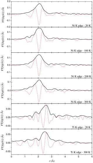
Figure 2: Magnitudes and imaginary parts of the Fourier transforms of the EXAFS $k\chi(k)$ data shown in fig. 1 for a-Ni₄₆Ti₅₄.

We made many tests considering different combinations of the experimental data and we will discuss here in details two models, defined as

Model A

all experimental data were used without constraints related to MSRD_⟂.

Model B

all experimental data were used together with the constraints related to MSRD_⟂.

To help the “visualization” of the possible constraints that can be introduced during the fitting process, fig. 3 presents a diagram showing all relations used in the various EXAFS analyses we made. In the diagram, $c_{i}$ is the concentration of atoms of type $i$, where $i=1$ for Ni and $i=2$ for Ti.

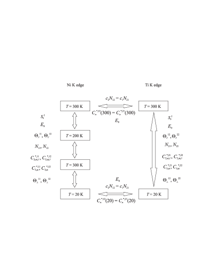
Figure 3: Diagram showing the possible constraints that can be used in the EXAFS analyses.

In Model A we did not consider any constraints for the first cumulant $C_{1}^{*}$ related to the MSRD_⟂, and we did not consider perpendicular Einstein temperatures. All other constraints shown in fig. 3 were introduced in order to decrease correlations. The cumulants $C_{2}^{*,ij}$ and $C_{3}^{*,ij}$ associated with each pair $ij$ were constrained to follow eqs. 17 and 18, respectively. Then, we obtained the threshold energy $E_{0}$, $N_{ij}$ (average coordination numbers), $C^{*,ij}_{2,{\text{st}},\parallel}$ and $C^{*,ij}_{3,{\text{st}}}$, $\Theta_{\parallel}^{ij}$, $k_{3}^{ij}$ and $C_{1}^{*,ij}=\langle r_{ij}\rangle$. Figure 4 shows the real parts of the Fourier filtered first shells obtained on Ni and Ti K edges. The agreement between the simulations and the experimental data is very good, and it happens for all measurements on both edges at all temperatures. Tables 1, 2 and 3 present the values obtained for the relevant quantities above considering model A, and fig. 5 shows the temperature dependence of $C_{2}^{*,ij}$ and $C_{3}^{*,ij}$ (see eqs. 17 and 18).

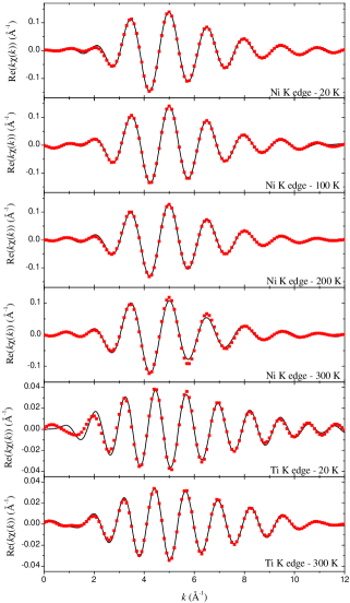
Figure 4: Real part of the Fourier filtered first shells of a-Ni₄₆Ti₅₄ (solid black lines) on Ni and Ti K edges at all temperatures investigated and their simulations (red squares).

Table 1: Average coordination numbers and structural components of cumulants $C^{*}_{2}$ and $C^{*}_{3}$ obtained from the EXAFS fits shown in fig. 4 for a-Ni₄₆Ti₅₄ considering model A.

Bond Type	$N$	$C^{*}_{2,{\text{st}}}$ ($\times 10^{-3}$ Å2)	$C^{*}_{3,{\text{st}}}$ ($\times 10^{-4}$ Å3)
Ni-Ni	$6.3\pm 1.0$	$5.3\pm 0.2$	$-0.72\pm 0.01$
Ni-Ti	$7.1\pm 0.6$	$15.1\pm 0.8$	$-4.2\pm 0.4$
Ti-Ti	$5.8\pm 0.3$	$3.1\pm 0.4$	$-1.4\pm 0.2$

Table 2: Parallel Einstein temperatures, parallel effective harmonic spring constants, parallel Einstein frequencies and cubic anharmonic force constants obtained from the EXAFS fits shown in fig. 4 for a-Ni₄₆Ti₅₄ considering model A.

Bond Type	$\Theta_{\parallel}$ (K)	$k_{e,\parallel}$ (eV/Å2)	$\nu_{\parallel}$ (THz)	$k_{3}$ (eV/Å3)
Ni-Ni	$251\pm 36$	3.3	5.2	$6.8\pm 1.5$
Ni-Ti	$326\pm 12$	5.0	6.8	$144\pm 5$
Ti-Ti	$257\pm 27$	2.8	5.4	$6.5\pm 2.3$

Table 3: First cumulant $C_{1}^{*,ij}$ obtained from the EXAFS fits shown in fig. 4 for a-Ni₄₆Ti₅₄ considering model A.

$T$ (K)	$C_{1}^{*,\text{Ni-Ni}}$ (Å)	$C_{1}^{*,\text{Ni-Ti}}$ (Å)	$C_{1}^{*,\text{Ti-Ti}}$ (Å)
20	$2.406\pm 0.004$	$2.447\pm 0.006$	$2.814\pm 0.003$
100	$2.413\pm 0.003$	$2.445\pm 0.005$	—
200	$2.418\pm 0.005$	$2.479\pm 0.006$	—
300	$2.455\pm 0.011$	$2.508\pm 0.005$	$2.852\pm 0.002$

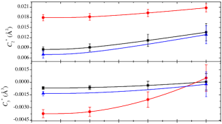
Figure 5: Cumulants $C_{2}^{*,ij}$ and $C_{3}^{*,ij}$ for a-Ni₄₆Ti₅₄ obtained for Ni-Ni (black squares), Ni-Ti (red circles) and Ti-Ti (blue triangles) as functions of temperature considering eqs. 17 and 18 respectively.

From Table 1 and fig. 5 it can be seen that the contribution of the parallel structural disorder $C_{2,\text{st},\parallel}^{*,ij}$ to the total MSRD_∥ is large, and it is the dominant factor even at 300 K for Ni-Ti pairs. We believe this fact can be associated with the fact that the sample is amorphous and also with fabrication technique used to produce the alloy. The third cumulant $C_{3}^{*,ij}$ indicates asymmetric distributions $\varrho_{ij}(r,T)$ at low temperatures due mainly to the contribution of the structural part since $C_{3,{\text{st}}}^{*,ij}$ is negative, but the asymmetry decreases with temperature. It is interesting to note the thermal behaviour of $C_{3}^{*,\text{Ni-Ti}}$, which is different from $C_{3}^{*,\text{Ni-Ni}}$ and $C_{3}^{*,\text{Ti-Ti}}$. This fact can be associated with the parallel Einstein temperatures obtained, since homopolar pairs have similar values and they are smaller than the value obtained for $\Theta_{\parallel}^{\text{Ni-Ti}}$ (see Table 2), and also with the anharmonicity of $V(r)$, indicated by the cubic anharmonic constants $k_{3}^{ij}$. The average interatomic distances (first cumulant) $C_{1}^{*,ij}$ indicate a thermal expansion for Ni-Ni and Ti-Ti pairs and a negative (although very small) thermal expansion for Ni-Ti pairs from 20 K to 100 K followed by a positive thermal expansion. From $\Delta C_{1}^{*,ij}$ the thermal expansion coefficients $\alpha_{ij}(T)$ can be estimated, and that will be done latter.

Now we can discuss model B. Since we had many constraints all structural values were obtained with enough accuracy to proceed to the next step. We fixed all values shown in Tables 1, 2 and 3 except $C_{1}^{*,ij}$, which were then constrained to follow eq. 11 with $\langle(\Delta u_{\perp}^{ij})^{2}\rangle$ given by eq. 19. Since we knew $C_{1}^{*,ij}$ from model A, we could analyze the new values obtained for $C_{1}^{*,ij}$ in order to avoid possible spurious results. The values obtained for the first cumulant were almost the same, and we were able to find $\Theta_{\perp}^{ij}$, $\text{MSRD}_{\perp}^{ij}$, $\langle\Delta u_{\parallel}^{ij}\rangle$, $R_{0}^{ij}$ and the corresponding amorphous distance $R_{a}^{ij}$ given by eq. 20. The fits obtained for model B are almost identical to those shown in Fig. 4 and will not be shown. Fig. 6 shows the thermal behavior of $C^{*,ij}_{\perp}$ given by eq. 19 and Fig. 7 compares the values obtained for $C_{1}^{*,ij}$ using models A and B. As it can be seen from Fig. 7 and also from Tables 3 and 4, the values obtained from both models are very similar. Table 5 shows other relevant structural parameters obtained.

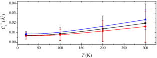
Figure 6: Cumulants $C_{\perp}^{*,ij}$ for a-Ni₄₆Ti₅₄ obtained for Ni-Ni (black squares), Ni-Ti (red circles) and Ti-Ti (blue triangles) as a function of temperature considering eq. 19.

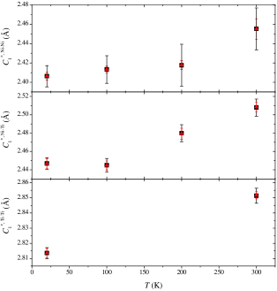
Figure 7: Comparison between cumulants $C_{1}^{*,ij}$ obtained from model A (red triangles) and model B (black squares).

Table 4: First cumulant $C_{1}^{*,ij}$ obtained from the EXAFS fits shown in Fig. 4 for a-Ni₄₆Ti₅₄ considering model B.

$T$ (K)	$C_{1}^{*,\text{Ni-Ni}}$ (Å)	$C_{1}^{*,\text{Ni-Ti}}$ (Å)	$C_{1}^{*,\text{Ti-Ti}}$ (Å)
20	$2.406\pm 0.011$	$2.447\pm 0.006$	$2.814\pm 0.004$
100	$2.413\pm 0.014$	$2.445\pm 0.007$	—
200	$2.418\pm 0.021$	$2.480\pm 0.009$	—
300	$2.455\pm 0.022$	$2.508\pm 0.009$	$2.851\pm 0.005$

Table 5: Rest distances $R_{0}^{ij}$, perpendicular Einstein temperatures, perpendicular effective harmonic spring constants and perpendicular Einstein frequencies obtained from the EXAFS fits for a-Ni₄₆Ti₅₄ considering model B.

Bond Type	$R_{0}^{ij}$ (Å)	$\Theta_{\perp}$ (K)	$k_{e,\perp}$ (eV/Å2)	$\nu_{\perp}$ (THz)
Ni-Ni	$2.400\pm 0.006$	$230\pm 121$	2.7	4.8
Ni-Ti	$2.438\pm 0.002$	$269\pm 140$	3.4	5.6
Ti-Ti	$2.810\pm 0.001$	$233\pm 52$	2.3	4.9

Due to similar $\Theta_{\perp}^{ij}$, the thermal behavior of $C^{*,ij}_{\perp}$ shown in Fig. 6 is similar. The perpendicular Einstein temperatures are smaller than the corresponding $\Theta_{\parallel}^{ij}$, the difference being larger for Ni-Ti pairs, indicating the presence of vibrational anisotropy for all pairs specially for Ni-Ti ones. The corresponding force constants and frequencies indicate a loosening of the perpendicular bond strengths when compared to the parallel ones. So, bending vibrational modes are more easily excited than stretching modes. Fig. 8 shows the ratio $\gamma_{ij}=C_{\perp}^{*,ij}/C_{2,\parallel,T}^{*,ij}$ obtained using eq. 17 and eq. 19. The values found are greater than 2, indicating the vibrational anisotropy, which is higher for the Ni-Ti pairs.

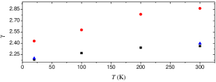
Figure 8: Ratio $\gamma_{ij}=C_{\perp}^{*,ij}/C_{2,\parallel,T}^{*,ij}$ obtained from EXAFS for Ni-Ni (black squares), Ni-Ti (red circles) and Ti-Ti (blue triangles) pairs in a-Ni₄₆Ti₅₄.

The values obtained for the first cumulants $C_{1}^{*,ij}$ shown in Fig. 7 and Tables 3 and 4 indicate a thermal expansion for Ni-Ni and Ti-Ti pairs for all temperatures and for Ni-Ti pairs after 100 K. However, these pairs seem to have a negative thermal expansion from 20 K to 100 K. Considering eqs. 11, 12 and 19, the perpendicular contribution $r_{\perp}^{ij}$ to $C_{1}^{*,ij}$ can be calculated and it is shown, together with the parallel contribution $r_{\parallel}^{ij}$, in Table 6.

Table 6: First cumulant $C_{1}^{*,ij}$ obtained from the EXAFS fits shown in Fig. 4 for a-Ni₄₆Ti₅₄ considering model B.

$T$ (K)	$r_{\parallel}^{\text{Ni-Ni}}$ (Å)	$r_{\perp}^{\text{Ni-Ni}}$ (Å)	$r_{\parallel}^{\text{Ni-Ti}}$ (Å)	$r_{\perp}^{\text{Ni-Ti}}$ (Å)	$r_{\parallel}^{\text{Ti-Ti}}$ (Å)	$r_{\perp}^{\text{Ti-Ti}}$ (Å)
20	$0.004\pm 0.005$	$0.0015\pm 0.0008$	$0.007\pm 0.004$	$0.0014\pm 0.0007$	$0.002\pm 0.002$	$0.0015\pm 0.0003$
100	$0.011\pm 0.007$	$0.002\pm 0.001$	$0.005\pm 0.004$	$0.002\pm 0.001$	—	$0.0019\pm 0.0006$
200	$0.014\pm 0.013$	$0.003\pm 0.003$	$0.039\pm 0.005$	$0.002\pm 0.002$	—	$0.003\pm 0.001$
300	$0.051\pm 0.012$	$0.004\pm 0.004$	$0.066\pm 0.004$	$0.003\pm 0.003$	$0.037\pm 0.002$	$0.004\pm 0.002$

From Table 6 it can be seen that the perpendicular contribution $r_{\perp}^{ij}$ associated with the rigid shift of the potential minimum is smaller than the term $r_{\parallel}^{ij}$, which is related to the anharmonicity and to the shape of the effective potential, and their difference increases as the temperature is raised. This fact suggests that the thermal expansion in a-Ni₄₆Ti₅₄ is caused mainly by changes in the shape of the potential and the rigid shift of the potential minimum is a secondary effect.

The thermal expansion coefficient $\alpha$ can be written as

$$\alpha(T)=\frac{1}{r}\frac{dr}{dt}=\frac{1}{C_{1}^{*}}\frac{dC_{1}^{*}}{dt}=\frac{1}{C_{1}^{*}}\frac{dr_{\parallel}}{dt}+\frac{1}{C_{1}^{*}}\frac{dr_{\perp}}{dt}=\alpha_{\parallel}+\alpha_{\perp}$$ (21)

The contribution $\alpha_{\perp}$ to the thermal expansion associated with perpendicular vibrations can be found exactly and typical values are $\alpha_{\perp}^{\text{Ni-Ni}}=5.1\times 10^{-6}$ K^-1 at 300 K and $\alpha_{\perp}^{\text{Ni-Ti}}=2.4\times 10^{-6}$ K^-1 at 100 K (the largest and the smallest values, respectively). The total thermal expansion can be estimated from $\Delta C_{1}^{*,ij}$ and, for Ni-Ti pairs at 100 K, it is negative and has the value $\alpha^{\text{Ni-Ti}}=-9.6\times 10^{-6}$ K^-1. All other values are positive and increase with temperature, ranging from $\alpha^{\text{Ni-Ni}}=3.6\times 10^{-5}$ K^-1, at 100 K, to $\alpha^{\text{Ni-Ni}}=1.5\times 10^{-4}$ K^-1, at 300 K. The contribution $\alpha_{\perp}$ to the total thermal expansion is always much smaller than $\alpha_{\parallel}$ except for Ni-Ti pairs at 100 K, indicating that the anharmonicity of the effective potencial is the dominant effect related to thermal expansion for the amorphous Ni₄₆Ti₅₄ alloy studied.

V Conclusion

We investigated the structure, anharmonicity, asymmetry of pair distribution functions, vibrational anisotropy and thermal expansion of an amorphous Ni₄₆Ti₅₄ alloy produced by mechanical alloying considering EXAFS data only. The detailed study described here was only possible due to the experimental data available on Ni and Ti K edges and at several temperatures, which allowed us to use many constraints to obtain reliable values for the cumulants $C_{1}^{*}$, $C_{2}^{*}$ and $C_{3}^{*}$, making it possible to extract the perpendicular contributions to the MSRD and $C_{1}^{*,ij}$. The method should also work for crystalline samples, but we believe that EXAFS measurements on edges of all atomic species present in the sample should be used. This procedure may be the only way to extract such structural information for amorphous samples, so more tests on other alloys would be important.

Concerning the Ni₄₆Ti₅₄ alloy, it presents asymmetric $\varrho_{ij}(r,T)$ functions at low temperatures due to the structural contribution but the asymmetry decreases with temperature until 300 K. After that, the asymmetry incrases again. There is vibrational anisotropy mainly for Ni-Ti pairs, indicating that bending modes are looser than stretching ones, and Ni-Ti pairs exhibits a negative thermal expansion around 100 K. It would be very interesting to study the crystalline shape memory NiTi phase in order to associate these properties with the mechanical properties of this alloy.