Nonlinear analysis of spacecraft thermal models

Abstract

We study the differential equations of lumped-parameter models of spacecraft thermal control. Firstly, we consider a satellite model consisting of two isothermal parts (nodes): an outer part that absorbs heat from the environment as radiation of various types and radiates heat as a black-body, and an inner part that just dissipates heat at a constant rate. The resulting system of two nonlinear ordinary differential equations for the satellite’s temperatures is analyzed with various methods, which prove that the temperatures approach a steady state if the heat input is constant, whereas they approach a limit cycle if it varies periodically. Secondly, we generalize those methods to study a many-node thermal model of a spacecraft: this model also has a stable steady state under constant heat inputs that becomes a limit cycle if the inputs vary periodically. Finally, we propose new numerical analyses of spacecraft thermal models based on our results, to complement the analyses normally carried out with commercial software packages.

Keywords: spacecraft thermal control, nonlinear oscillations, perturbation methods

1 Introduction

The thermal analysis of a spacecraft is important to ensure that the temperatures of its elements are kept within their appropriate ranges [1, 2, 3, 4, 5]. This analysis is usually carried out numerically by commercial computer software packages. These software packages employ “lumped parameter” models that describe the spacecraft as a discrete network of nodes, with one heat-balance equation per node. The equations for the thermal state evolution are coupled nonlinear first order differential equations, which can be integrated numerically. Given the thermal parameters of the model and its initial state, the numerical integration of the differential equations provides the solution of the problem, namely, it yields the evolution of the node temperatures. However, it does not provide any information on the qualitative behavior of the set of solutions nor knowledge of the response of the model to changes in the parameter values. Besides, a detailed model with many nodes is difficult to handle, and its integration for a sufficiently long time of evolution can take considerable computer time and resources. Therefore, it is very useful to study, on the one hand, simplified models with few nodes that lend themselves to analytic solutions, and, on the other hand, the reduction of complex models to simpler ones. These studies are especially helpful early in the design process, when the concept of the spacecraft is still open, and also at the end of the process, to simplify the full thermal model for the final assessment of the mission.

The differential equations for heat balance are nonlinear due to the presence of radiative couplings, which involve the fourth powers of the temperatures (according to the Stefan-Boltzmann law of thermal radiation). The computation of steady states, in particular, boils down to the solution of a set of fourth-degree algebraic equations. Most analytical approaches to the solution of the heat balance equations, either for transient or steady states, involve a sort of linearization of the radiative couplings such that they become analogous to conductive couplings [6, 7, 8, 9, 10]. But one must beware that the “radiative conductances” so defined actually depend on the temperatures (the unknown variables). Therefore, the linearization procedure is sound only when those radiative conductances can be considered constant, namely, when the temperatures are sufficiently close to their steady state values. We can see, in particular, that the linear equations are not suitable for calculating the steady state values of the temperatures. Moreover, one may question that the steady state is unique. Even assuming that it is and that the steady state temperatures are known, the linear equations are not suitable in the presence of variable external heat inputs of such a magnitude that they make the node temperatures depart considerably from their steady state values.

For the given reasons, it is advisable to study the full nonlinear equations and only consider their linearization once we have a qualitative understanding of the possible behavior of their solutions. This is the philosophy applied in our preceding work [11]. The present work continues the development of nonlinear analytic methods for the study of simple models of spacecrafts (in particular, satellites) that we have begun in Ref. [11]. We study there the simplest model, namely, a one-node (isothermal) model. In that case, the steady state temperature is obtained at once, the heat-balance equation without external heat input is integrable in terms of known functions, and the equation with periodic external heat input admits a full qualitative analysis. Naturally, as we increase the number of nodes, the corresponding systems of equations become increasingly difficult to handle. Indeed, a two-node model is already of such a complexity that the existing studies of this model are based on some sort of linearization: Oshima & Oshima [6] assume radiative conductances that depend on a temperature $T_{0}$ that is “to be defined in each problem,” whereas Pérez-Grande et al [10] choose the temperature on which the conductance between two nodes depends to be an average of the two nodes temperatures. Thus, Pérez-Grande et al’s radiative conductances are not really constant. In any event, both procedures are somewhat arbitrary and, in fact, only agree if the temperatures are sufficiently close to their steady state values and, in addition, all the temperatures are almost equal in the steady state.

The purpose of the present study is to provide a nonlinear analysis of a two-node model of a small compact satellite in a low orbit and to generalize this analysis to a many-node thermal model of a spacecraft. We employ Pérez-Grande et al’s two-node satellite model [10], in which the two nodes are formed by the satellite’s interior and its outer shell (its “skin”). Therefore, the model consists in a system of two energy-balance ordinary differential equations (ODE’s), in which both nodes are thermally coupled to one another but only the outer shell radiates heat away. Naturally, this two-node model is more general than the one-node model studied in Ref. [11], but it reduces to the latter if the thermal coupling between the satellite’s interior and its outer shell is strong, as we show here. On the other hand, if the thermal coupling is weak, the two-node model can significantly differ from the one-node model. In fact, the corresponding system of two non-autonomous ODE’s for this two-node model under periodic heat input is equivalent to an autonomous system of three ODE’s, to which the qualitative methods of Ref. [11] are not applicable and which could have chaotic behavior and very complicated attractors, as is well known [12, 13]. We consider this possibility here.

A general many-node thermal model of a spacecraft consists in a system of many energy-balance ODE’s. As a first step in this generalization, we find it useful to study the general two-node model in which both nodes radiate heat away. This model already requires the use of sophisticated mathematical methods, but its temperature space is still two-dimensional, allowing us to obtain stronger results than for the fully general case. The fully general many-node thermal model presents some difficulties already in a linear analysis, for we have to deal with nontrivial high-dimensional matrices.

An important issue in the study of a differential equation is the stability of its solutions. As regards autonomous equations, it is important to determine the stability of their equilibrium states (steady states). For non-autonomous equations, one may consider the more general question of the stability of a given trajectory under a perturbation of the initial conditions, where stability is normally interpreted in the sense of Lyapunov [13]. A different notion of stability is structural stability, which refers to the entire set of solutions and means that its qualitative character is “robust” against perturbations [12, 13]. We study the stability of the heat balance equations, namely, the question of the stability of the steady states of the autonomous equations and the related question of the stability of the limit cycle of the general equations with periodic heat input. We also study the structural stability of the equations under a variation of the heat inputs.

Thus, our goal is to carry out a fairly complete study of the lumped parameter thermal models employed in the thermal analysis of spacecrafts. Pérez-Grande et al’s two-node satellite model is studied in Sect. 2, where the energy balance equations are formulated as a system of two non-dimensional ODE, which are nonlinear and non-autonomous. Then, we consider an autonomous system that plays the role of a time average of the actual system. The analysis of the autonomous system begins with the calculation of its steady states, finding only a physically relevant one, namely, a stable sink of the ODE system’s flow. Two examples with different parameters, corresponding to strong and weak thermal coupling, are solved numerically. After introducing the thermal driving, we employ a perturbation method that generalizes the method in Ref. [11] and we corroborate its results numerically. In Sect. 3, we introduce the general $N$-node model and then study the corresponding autonomous system, beginning with the general two-node model. We prove that the results for the restricted two-node model hold for the general two-node model and, furthermore, that most of those results can be extended to the general $N$-node model. Finally, we present our conclusions, regarding the design of spacecraft.

2 Two-node model of a satellite

A lumped-parameter thermal model of a continuous system describes the system as a discrete network of isothermal regions (nodes) that represent a partition of the thermal capacitance of the system and that are linked by conductive and radiative thermal couplings [1, 2, 3, 4, 5, 6]. The equation governing the conductive heat transfer is the standard Fourier partial differential equation. This PDE is actually employed for thermal modelling of simple spacecraft geometries, treating the external radiative heat input and heat dissipation as boundary conditions [9]. However, when we consider the radiative thermal coupling between different parts of a spacecraft, we have a much more complex situation: the internal radiative couplings are not a boundary condition and are non-local, thus giving rise to an integro-differential equation for the heat transfer. The discretization of this equation in terms of a lumped-parameter model is a very convenient approach.

In a lumped-parameter thermal model, there is one heat-balance ODE per node controlling the evolution of its temperature. A single-node model, suitable for a small and compact satellite, has been first studied by Oshima & Oshima [6] and has been revisited by Tsai [8]. Oshima & Oshima [6] also study the two-node model, but they linearize it from the outset and assume constant heat inputs. Here, we focus on Pérez-Grande et al’s two-node satellite model [10], with one node corresponding to the satellite’s outer shell and the other to its interior. This model allows for a periodic time dependence of the heat inputs. To be precise, the heat input to the satellite’s shell consists, on the one hand, of the periodic solar irradiation and the planetary albedo, and, on the other hand, of the constant planetary IR radiation. The internal heat is due to the equipment dissipation and is taken constant. Let $T_{\mathrm{e}}$ and $T_{\mathrm{i}}$ denote, respectively, the outer and inner node temperatures; then, the energy balance equations for them are

$$C_{\mathrm{e}}\,\dot{T_{\mathrm{e}}} = \dot{Q}_{\mathrm{s}}\,f_{\mathrm{s}}(\nu t)+\dot{Q}_{\mathrm{a}}\,f_{\mathrm{a}}(\nu t)+\dot{Q}_{\mathrm{p}}+K_{\mathrm{ie}}(T_{\mathrm{i}}-T_{\mathrm{e}})+R_{\mathrm{ie}}(T_{\mathrm{i}}^{4}-T_{\mathrm{e}}^{4})-A\varepsilon\sigma\,T_{\mathrm{e}}^{4},$$ (1)

$$C_{\mathrm{i}}\,\dot{T_{\mathrm{i}}} = \dot{Q}_{\mathrm{i}}+K_{\mathrm{ie}}(T_{\mathrm{e}}-T_{\mathrm{i}})+R_{\mathrm{ie}}(T_{\mathrm{e}}^{4}-T_{\mathrm{i}}^{4}).$$ (2)

Here $C_{\mathrm{e}}$ and $C_{\mathrm{i}}$ are the thermal capacities of the two satellite’s nodes, $\nu$ is the orbital frequency, $K_{\mathrm{ie}}$ and $R_{\mathrm{ie}}$ are the conductive and radiative couplings, respectively, $A$ is the satellite’s surface area, $\varepsilon$ its emissivity, and $\sigma$ is the Stefan-Boltzmann constant. The heat inputs are written as $\dot{Q}$ with a subscript that denotes their type, namely, solar irradiation, albedo, planetary IR radiation, or internal heat dissipation. The functions $f_{\mathrm{s}}$ and $f_{\mathrm{a}}$ are periodic with period one and give the time variations of the respective heat inputs.

Following Refs. [10, 11], we assume that $f_{\mathrm{s}}$ and $f_{\mathrm{a}}$ are given by:

$$f_{s}(x)=1,\;0\leq x\leq x_{1}\;{\rm or}\;1-x_{1}\leq x\leq 1;\;f_{s}(x)=0,\;x_{1}<x<1-x_{1};$$

$$f_{a}(x)=\cos(2\pi x),\;0\leq x\leq x_{2}\;\textrm{or}\;1-x_{2}\leq x\leq 1;\;f_{a}(x)=0,\;x_{2}\leq x\leq 1-x_{2};$$

$$f_{s,a}(x)=f_{s,a}(x-1),\;x\geq 1.$$

The values of $f_{s}$, alternating between one and zero, correspond to the orbit in the sunshine or eclipse, respectively. The fraction of the period in the sunshine or eclipse is determined by $x_{1}$, which is smaller than one half. Its value depends on the angle between the orbital plane and the solar vector [1, 2, 4]. The albedo heat input has a more complex time dependence, due to the change of the view factor from the whole satellite to the lit side of the planet along the orbit: the maximum albedo occurs at the minimum angle between the satellite’s local vertical and the solar vector, and it diminishes as the angle grows. The sinusoidal dependence assumed for $f_{a}$ is a suitable approximation of the actual dependence [2]. One must further assume that the fraction of the period with albedo heat input, namely, $2x_{2}$, is such that $x_{2}<x_{1}$.

The solar irradiation heat input to the satellite is the product of the solar constant, the satellite surface’s absorptivity and its projected area (which we take to be a quarter of its total area); namely,

$$\dot{Q}_{\mathrm{s}}=G_{\mathrm{s}}\,\alpha_{\mathrm{s}}\,A/4\,.$$

The albedo varies with time, as the atmospheric conditions and other factors change, so one must consider an average value. To calculate $\dot{Q}_{\mathrm{a}}$, it is necessary, in addition, to consider the already mentioned view factor, for the reflected light does not impinge on the satellite uniformly. This has the consequence of reducing the effective area to about a half of its nominal value when the sun is just above the satellite. Therefore, the maximum albedo heat input is $\dot{Q}_{\mathrm{a}}=2a\,\dot{Q}_{\mathrm{s}}\,,$ where $a$ denotes the average albedo coefficient. The planetary IR irradiation heat input is given by

$$\dot{Q}_{\mathrm{p}}=(A/2)\varepsilon\sigma\,T_{\mathrm{p}}^{4}\,,$$

where $T_{\mathrm{p}}$ is the planet’s (Earth’s) blackbody-equivalent temperature, the projected area is a half of the real area (like for albedo absorption), and the satellite’s surface IR absorptivity is taken equal to its IR emissivity $\varepsilon$. The value of $T_{\mathrm{p}}$ derives from the planet’s heat balance equation [1]

$$4\sigma T_{\mathrm{p}}^{4}=(1-a)\,G_{\mathrm{s}}\,.$$

The standard value of the average albedo coefficient of the Earth is $a=0.3$, which gives $\sigma\,T_{\mathrm{p}}^{4}=239.7\;\mathrm{W}\mathrm{m}^{-2}$ (using the value of $G_{\mathrm{s}}$ in Table 1). In conclusion, the IR irradiation heat input can be computed with the formula:

$$\dot{Q}_{\mathrm{p}}=\varepsilon A\,(119.9\;\mathrm{W}\mathrm{m}^{-2}).$$ (3)

Pérez-Grande et al’s two-node thermal model is applicable to micro-satellites. Specifically, we have in mind a micro-satellite with the shape of a cube of $0.5$ m side and with mass of about 50 kg, mostly covered by solar cells. The relevant values of the satellite and orbital parameters for two model examples are collected in Table 1 and employed in Sects. 2.3 and 2.6.

We can write equations (1) and (2) in a non-dimensional form by defining

$$b = A\varepsilon\sigma/(C_{\mathrm{e}}\nu),$$

$$q_{\mathrm{s}} = b^{1/3}\,\dot{Q}_{\mathrm{s}}/(C_{\mathrm{e}}\nu),\quad q_{\mathrm{a}}=b^{1/3}\,\dot{Q}_{\mathrm{a}}/(C_{\mathrm{e}}\nu),$$

$$q_{\mathrm{p}} = b^{1/3}\,\dot{Q}_{\mathrm{p}}/(C_{\mathrm{e}}\nu),\quad q_{\mathrm{i}}=b^{1/3}\,\dot{Q}_{\mathrm{i}}/(C_{\mathrm{e}}\nu),$$

$$k = K_{\mathrm{ie}}/(C_{\mathrm{e}}\nu),\quad r=R_{\mathrm{ie}}/(C_{\mathrm{e}}\nu\,b),$$

$$c = C_{\mathrm{i}}/C_{\mathrm{e}}\,,$$

and defining non-dimensional temperature variables

$$\theta_{\mathrm{e}}=b^{1/3}\,T_{\mathrm{e}}\,,\;\theta_{\mathrm{i}}=b^{1/3}\,T_{\mathrm{i}}\,,$$

and a time variable $\nu t$ (which is still denoted by $t$ for notational simplicity). Thus, we obtain the non-dimensional ODE’s

$$\dot{\theta}_{\mathrm{e}} = q_{\mathrm{p}}+q_{\mathrm{s}}\,f_{s}(t)+q_{\mathrm{a}}\,f_{a}(t)+k(\theta_{\mathrm{i}}-\theta_{\mathrm{e}})+r(\theta_{\mathrm{i}}^{4}-\theta_{\mathrm{e}}^{4})-\theta_{\mathrm{e}}^{4},$$ (4)

$$c\,\dot{\theta}_{\mathrm{i}} = q_{\mathrm{i}}+k(\theta_{\mathrm{e}}-\theta_{\mathrm{i}})+r(\theta_{\mathrm{e}}^{4}-\theta_{\mathrm{i}}^{4}).$$ (5)

This system of two non-autonomous nonlinear ODE’s is difficult to solve. As a first step, we remove the oscillating terms by averaging $f_{\mathrm{s}}$ and $f_{\mathrm{a}}$, like in Ref. [11].

2.1 Steady state temperatures

If $q_{\mathrm{e}}$ denotes the time average of the external heat input $q_{\mathrm{p}}+q_{\mathrm{s}}\,f_{\mathrm{s}}(t)+q_{\mathrm{a}}\,f_{\mathrm{a}}(t)$, then the averaging of the dynamical equations (4) and (5) results in the autonomous system:

$$\dot{\theta}_{\mathrm{e}} = q_{\mathrm{e}}+k(\theta_{\mathrm{i}}-\theta_{\mathrm{e}})+r(\theta_{\mathrm{i}}^{4}-\theta_{\mathrm{e}}^{4})-\theta_{\mathrm{e}}^{4},$$ (6)

$$c\,\dot{\theta}_{\mathrm{i}} = q_{\mathrm{i}}+k(\theta_{\mathrm{e}}-\theta_{\mathrm{i}})+r(\theta_{\mathrm{e}}^{4}-\theta_{\mathrm{i}}^{4}).$$ (7)

Instead of the one-node model averaged equation [11], which is straightforward to solve, we have now a system of two autonomous nonlinear ODE’s. The standard way of analyzing these systems begins with the localization of their fixed points [18].

The fixed points of Eqs. (6) and (7) are the solutions of two fourth degree algebraic equations. These two equations can be solved by first eliminating one unknown, namely, $\theta_{\mathrm{i}}$, as is easily done by adding both equations, which yields $\theta_{\mathrm{e}}^{4}=q_{\mathrm{e}}+q_{\mathrm{i}}$. Thus, the outer node temperature is given by $\theta_{\mathrm{e}}=(q_{\mathrm{e}}+q_{\mathrm{i}})^{1/4}$. It only depends on the total heat input, like the steady state temperature in the one-node model [11]. Once $\theta_{\mathrm{e}}$ is known, we can substitute for it in one of the algebraic equations, say the second one, to obtain a fourth degree algebraic equation for $\theta_{\mathrm{i}}\,,$ namely,

$$q_{\mathrm{i}}+k\theta_{\mathrm{e}}+r\theta_{\mathrm{e}}^{4}-k\theta_{\mathrm{i}}-r\theta_{\mathrm{i}}^{4}=0.$$ (8)

According to the fundamental theorem of algebra [14], this equation has four complex roots (solutions), of which an even number (0, 2 or 4) are real. We are interested in just the real positive roots. To this end, we apply Descartes’s rule of signs, which says that no equation can have more positive roots than it has changes of signs in the coefficients [15]. Clearly, there is only one change of sign, so there is one positive root at the most. If we replace $\theta_{\mathrm{i}}\rightarrow-\theta_{\mathrm{i}}$ in the equation, we also deduce that there is one negative root at the most. Therefore, the equation can have a positive and a negative root or no real roots at all. Given that the corresponding polynomial is positive for $\theta_{\mathrm{i}}=0$ and becomes negative as $\left|\theta_{\mathrm{i}}\right|\rightarrow\infty$, there is at the least one real root. Thus, the equation must have a positive and a negative root, in addition to a pair of complex conjugate roots.

The equation $\theta_{\mathrm{e}}^{4}=q_{\mathrm{e}}+q_{\mathrm{i}}$ also has a positive root, a negative root, and a pair of complex conjugate roots, but these are just the four complex fourth roots of a positive real number. When we consider the two fourth-degree equations together, the total number of roots is $4\times 4=16$, but only one has positive $\theta_{\mathrm{e}}$ and $\theta_{\mathrm{i}}$ . The positive root of Eq. (8) has a complicated expression in terms of radicals of the coefficients of the equation [14, 15]. Assuming that the coefficients have numerical values, it is much more convenient to find the root by numerical methods.

The existence of one and only one couple of positive steady-state temperatures is, of course, in accord with our physical intuition. In fact, one may wonder why there are other real solutions with negative absolute temperatures and why the flow given by Eqs. (6) and (7) crosses the axes $\theta_{\mathrm{e}}=0$ or $\theta_{\mathrm{i}}=0$. In this regard, let us notice that those equations are not valid when $\theta_{\mathrm{e}}$ or $\theta_{\mathrm{i}}$ vanish, because the thermal capacities $C_{\mathrm{e}}$ and $C_{\mathrm{i}}$ can only be taken constant in an interval of temperatures, which is usually long but cannot be extended to zero absolute temperature. In fact, the third law of thermodynamics implies that any thermal capacity vanishes as the absolute temperature approaches zero [16].

2.2 Stability of the steady state

To determine the stability of the steady state we have to calculate the Jacobian matrix of the vector field defined by the ODE’s [13, 18, 21], namely, of the vector field

$$\left\{q_{\mathrm{e}}+k(\theta_{\mathrm{i}}-\theta_{\mathrm{e}})+r(\theta_{\mathrm{i}}^{4}-\theta_{\mathrm{e}}^{4})-\theta_{\mathrm{e}}^{4}\,,\;c^{-1}\left[q_{\mathrm{i}}+k(\theta_{\mathrm{e}}-\theta_{\mathrm{i}})+r(\theta_{\mathrm{e}}^{4}-\theta_{\mathrm{i}}^{4})\right]\right\}.$$ (9)

If the Jacobian matrix is nonsingular, the fixed point is simple and the signs of the eigenvalues of the Jacobian matrix determine the nature and stability of the fixed point. In particular, if both eigenvalues are negative or, more generally, have negative real parts, the fixed point is an asymptotically stable sink, at least, locally.

The Jacobian matrix

$$J=\left(\begin{array}[]{cc}-k-4(r+1)\theta_{\mathrm{e}}^{3}&k+4r\theta_{\mathrm{i}}^{3}\\ \left(k+4r\theta_{\mathrm{e}}^{3}\right)/c&\left(-k-4r\theta_{\mathrm{i}}^{3}\right)/c\end{array}\right).$$ (10)

is indeed nonsingular, for

$$\det J=J_{11}J_{22}-J_{12}J_{21}=\frac{4\,\theta_{\mathrm{e}}^{3}\left(k+4r\theta_{\mathrm{i}}^{3}\right)}{c}>0.$$

The eigenvalue equation

$$(J_{11}-\l)(J_{22}-\l)-J_{12}J_{21}=J_{11}J_{22}-J_{12}J_{21}-(J_{11}+J_{22})\l+\l^{2}=0$$

has discriminant

$$\Delta=(J_{11}+J_{22})^{2}-4(J_{11}J_{22}-J_{12}J_{21})=(J_{11}-J_{22})^{2}+4J_{12}J_{21}\,.$$ (11)

It is positive, given that $J_{12}J_{21}>0$. Therefore, both eigenvalues are real and different. This implies that the matrix $J$ is diagonalizable. The larger eigenvalue

$$\l=\frac{1}{2}\left(J_{11}+J_{22}+\sqrt{\Delta}\right)$$

is negative if $\sqrt{\Delta}<-(J_{11}+J_{22})$, that is to say, if $\Delta<(J_{11}+J_{22})^{2}$, equivalent to $J_{11}J_{22}-J_{12}J_{21}>0$. In consequence, both eigenvalues are negative, so the fixed point is a stable sink and, to be specific, it is a node.

The local asymptotic stability of the fixed point is, again, in accord with our physical intuition. Furthermore, we expect that the fixed point be a global sink in the positive temperature quadrant. This can be proved with the help of Bendixson’s criterion [18]: if on a simple connected region the divergence of the ODE’s vector field does not change sign, then the ODE’s has no closed trajectories lying entirely in that region. This criterion is applicable, for the divergence equals $J_{11}+J_{22}$, which is always negative in the positive temperature quadrant. The absence of closed trajectories must be combined with the Poincaré-Bendixson theorem [18, 21, 13], which restricts the generic behavior of an autonomous system of two first-order ODE’s to having “simple” attracting sets, namely, fixed points or limit cycles. On account of the trivial fact that the flow points towards the interior of the positive temperature quadrant, we conclude that the flow must end at its unique sink in the quadrant, which is therefore globally stable in it.

2.3 Numerical examples

After establishing that the flow has a globally stable sink, it is useful to see the aspect of the flow for sensible values of the parameters by plotting the ODE’s vector field (9). In addition, the computation of the eigenvalues and eigenvectors of the respective Jacobian matrices provides a very precise local picture of the flow around the fixed points. that confirms and completes the global picture provided by the vector fields. We examine two examples: one in which the two nodes are strongly coupled (large values of $K_{\mathrm{ie}}$ and $R_{\mathrm{ie}}$) and another in which the coupling is weak (small $K_{\mathrm{ie}}$ and $R_{\mathrm{ie}}$). The corresponding values of all the parameters are given in Table 1.

	Example 1	Example 2
Outer node area $A$ (m2)	$1.5$	idem
Outer node heat capacity $C_{\mathrm{e}}$ (J K-1)	18 000	idem
Inner node heat capacity $C_{\mathrm{i}}$ (J K-1)	13 500	24 000
Conductance $K_{\mathrm{ie}}$ (W K-1)	10	1
Radiative coupling constant $R_{\mathrm{ie}}$ (W K-4)	$3.6\cdot 10^{-8}$	$9\cdot 10^{-9}$
Solar absorptivity $\alpha_{\mathrm{s}}$	0.8	idem
Emissivity $\varepsilon$	0.7	idem
Internal heat dissipation (W)	40	80
Solar constant $G_{\mathrm{s}}$ (W m-2)	1 370	idem
Earth’s albedo coefficient $a$	0.3	idem
Orbital frequency $\nu$	(1.5 h)-1	idem
Solar time fraction $2x_{1}$	0.6	idem
Albedo time fraction $2x_{2}$	0.5	idem

Table 1: Satellite and orbital parameters for two numerical examples.

2.3.1 Example 1: strong coupling

From the parameters in Table 1, we can obtain the non-dimensional parameters as follows. We first calculate the denominator $C_{\mathrm{e}}\,\nu=18\hskip 1.0pt000\,\mathrm{JK}^{-1}\,(1.5\cdot 3600\,\mathrm{s})^{-1}=3.333$ W K^-1, and then calculate:

$$b = \frac{1.5\cdot 0.7\cdot 5.67\cdot 10^{-8}}{3.333}\,\mathrm{K}^{-3}=1.786\cdot 10^{-8}\,\mathrm{K}^{-3},$$

$$k = \frac{10}{3.333}=3,\quad r=\frac{3.6\cdot 10^{-8}\,\mathrm{K}^{-3}}{3.333\,b}=0.6047,$$

$$q_{\mathrm{s}} = b^{1/3}\frac{1370\cdot 0.8\cdot 1.5/4}{3.333\,\mathrm{K}^{-1}}=0.3223,\quad q_{\mathrm{i}}=\frac{40\,b^{1/3}}{3.333\,\mathrm{K}^{-1}}=0.03137,\quad c=\frac{13\hskip 1.0pt500}{18\hskip 1.0pt000}=0.75.$$

To calculate $q_{\mathrm{e}}$ we need the average of the periodic functions $f_{\mathrm{s}}$ and $f_{\mathrm{a}}$, which yields $q_{\mathrm{e}}=q_{\mathrm{p}}+2x_{1}q_{\mathrm{s}}+q_{\mathrm{a}}/\pi$ [11]. We have that $q_{\mathrm{a}}=2aq_{\mathrm{s}}=0.6\cdot 0.3223=0.1934$, and, on account of Eq. (3),

$$q_{\mathrm{p}}=\frac{b^{1/3}(0.7\cdot 1.5\cdot 119.9)}{3.333\,\mathrm{K}^{-1}}=0.09872,$$

so that

$$q_{\mathrm{e}}=0.09872+0.6\cdot 0.3223+0.1934/\pi=0.3537.$$

With the given values of the non-dimensional parameters, we can compute the fixed point by using, for example, Newton’s method, with initial values $\theta_{\mathrm{e}}=\theta_{\mathrm{i}}=1$. The solution is $\theta_{\mathrm{e}}^{*}=0.7877,\;\theta_{\mathrm{i}}^{*}=0.7952$ (to which correspond $T_{\mathrm{e}}^{*}=301.4~{}\mathrm{K},\;T_{\mathrm{i}}^{*}=304.2~{}\mathrm{K}$). We can also compute the eigenvalues of the Jacobian matrix at $\left(\theta_{\mathrm{e}}^{*},\theta_{\mathrm{i}}^{*}\right)$, which must be negative, according to Sect. 2.2. The computation of the eigenvalues yields $\{-10.74,-1.024\}$, which are indeed negative; besides, they are very different in absolute value, due to the magnitude of the discriminant $\Delta$ (11). Therefore, the flow converges to the node much faster in the direction of the eigenvector corresponding to the eigenvalue $-10.74$ than in the direction of the eigenvector corresponding to $-1.024$. The former eigenvector is $(-0.6759,0.7370)$ (or a multiple thereof), whereas the latter is $(0.6362,0.7716)$. The consequent local flow pattern is borne out by the plot of the vector field flow in the square $[0,2]\times[0,2]$ that is shown in Fig. 1.

Figure 1: Temperature flow of a model with strong coupling. The steady state is marked by a dot. Multiplying $\theta_{\mathrm{e}}$ and $\theta_{\mathrm{i}}$ by $b^{-1/3}=382.6$ K one obtains the absolute temperatures $T_{\mathrm{e}}$ and $T_{\mathrm{i}}$.

The qualitative features of the flow can be deduced from the results in Sects. 2.1 and 2.2. As the coupling parameters $k$ and $r$ are large in comparison with the heat input $q_{\mathrm{i}}$, we can make $q_{\mathrm{i}}=0$ in Eq. (8) for $\theta_{\mathrm{i}}$, which implies that $\theta_{\mathrm{i}}=\theta_{\mathrm{e}}$. Notice that any $q_{\mathrm{i}}>0$ gives rise to $\theta_{\mathrm{i}}>\theta_{\mathrm{e}}$, as is natural on physical grounds. Thus, we put $\theta_{\mathrm{i}}=\theta_{\mathrm{e}}+\delta$ in Eq. (8), expand it to first order in $\delta$, and solve the resulting linear equation for $\delta$ to obtain

$$\delta=\frac{q_{\mathrm{i}}}{k+4r\theta_{\mathrm{e}}^{3}}\,.$$

The resulting numerical value $\delta\simeq 0.0075$ coincides with the difference $\theta_{\mathrm{i}}^{*}-\theta_{\mathrm{e}}^{*}$ found in the numerical computation. As regards the Jacobian matrix $J$ and the discriminant $\Delta$, given by Eqs. (10) and (11), respectively, we can make in these equations $\theta_{\mathrm{i}}=\theta_{\mathrm{e}}=0.7877$. Thus, the discriminant

$$\Delta=(J_{11}-J_{22})^{2}+4J_{12}J_{21}\simeq 93.6.$$

This yields a difference between eigenvalues $\sqrt{\Delta}\simeq 9.7$, which is very close to the already found value. Of course, the large value of $\sqrt{\Delta}$ is the cause of the appearance of a “fast variable” and a “slow variable”, such that the flow is first attracted to the almost diagonal curve in Fig. 1, along which it flows towards the fixed point. Therefore, the temperatures of the two nodes quickly become approximately equal and then the common temperature evolves towards its steady value. This type of evolution justifies the isothermal model studied in Ref. [11].

2.3.2 Example 2: weak coupling

As a second example, we consider smaller values of the thermal couplings between nodes. In practice, the conductance $K_{\mathrm{ie}}$ can be substantially reduced through a reduction of the joints between the satellite’s core and its outer shell, in addition to the use of thermally insulating material. The radiative coupling $R_{\mathrm{ie}}$ can also be reduced by using materials with low absorptivities and emissivities for the relevant surfaces. The new values of $K_{\mathrm{ie}}$ and $R_{\mathrm{ie}}$ are displayed in the last column of Table 1. On the other hand, as seen in the table, we assume larger internal heat capacity and dissipation, to enhance the differences with the preceding example.

Among the five non-dimensional parameters entering in Eqs. (6) and (7), the non-dimensional external heat input keeps its former value, namely, $q_{\mathrm{e}}=0.3537$, but $k,\,r,\,q_{\mathrm{i}}$ and $c$ adopt new values, namely,

$$k=0.3,\quad r=0.1512,\quad q_{\mathrm{i}}=0.06274,\quad c=1.333.$$

Using these values, we compute the fixed point (with Newton’s method and starting with the same initial values $\theta_{\mathrm{e}}=\theta_{\mathrm{i}}=1$); we obtain $\theta_{\mathrm{e}}^{*}=0.8033,\;\theta_{\mathrm{i}}^{*}=0.8966$ (to which correspond $T_{\mathrm{e}}^{*}=307.3~{}\mathrm{K},\;T_{\mathrm{i}}^{*}=343.0~{}\mathrm{K}$). We obtain the eigenvalues $\{-2.835,-0.4036\}$ and the respective eigenvectors $(-0.9803,0.1975)$ and $(0.3067,0.9518)$. The eigenvalues are not as different in absolute value as in the preceding example (now $\sqrt{\Delta}=2.432$). Nevertheless, the convergence is still considerably slower in the $(0.3067,0.9518)$ direction.

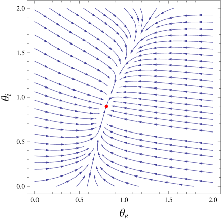
Figure 2: Temperature flow of a model with weak coupling. Multiplying $\theta_{\mathrm{e}}$ and $\theta_{\mathrm{i}}$ by $382.6$ K one obtains $T_{\mathrm{e}}$ and $T_{\mathrm{i}}$.

The flow in the square $[0,2]\times[0,2]$ is shown in Fig. 2. Since there is a relatively fast variable, the flow is again initially attracted to a curve; but now this curve, which approximately goes along the eigenvector $(0.3067,0.9518)$, is not close to the diagonal. In fact, for some initial values of the temperatures, the difference between the two temperatures oscillates, taking both signs (the trajectory crosses the diagonal). Notice that the reduction to an isothermal model is not appropriate in the weakly coupled case.

We remark that it is possible to reduce further the value of the discriminant $\Delta$ while keeping $q_{\mathrm{e}}>0,\,q_{\mathrm{i}}>0,\,k>0,\,r>0$ and $c>0.$ In fact, keeping $q_{\mathrm{e}}=0.3537$, one can get $\Delta\simeq 0.02$ for small values of the other parameters (especially, $k$ and $r$ but also $c$ and $q_{\mathrm{i}}$). Thus, there are no fast and slow variables. However, those small values of $k,\,r,\,c$ and $q_{\mathrm{i}}$ correspond to hardly realizable values of the physical parameters.

2.4 Driven two-node model

In this section, we study the original Eqs. (4) and (5), without averaging the periodic driving term $q_{\mathrm{p}}+q_{\mathrm{s}}\,f_{\mathrm{s}}(t)+q_{\mathrm{a}}\,f_{\mathrm{a}}(t).$ As in Ref. [11], it is convenient to redefine this term as

$$f(t)=q_{\mathrm{p}}+q_{\mathrm{s}}\,f_{\mathrm{s}}(t)+q_{\mathrm{a}}\,f_{\mathrm{a}}(t)-q_{\mathrm{e}}\,,$$ (12)

such that it has vanishing average over a period and represents the deviations about the mean. The addition of $f(t)$ converts the autonomous system of the two ODE’s (6) and (7) in an autonomous system of three ODE’s, the third equation being $\dot{t}=1$ (the new system is called the suspended system). Three-dimensional autonomous systems can have very complex flows as is well known; in particular, they and can have chaotic attractors [12, 13].

Complex three-dimensional flows, in particular, chaotic flows, can arise from simpler flows through instabilities and bifurcations. Drazin [13] distinguishes four routes to chaos, three of which can operate in our case. (i) subcritical instability, (ii) a sequence of bifurcations, (iii) period doubling, and (iv) intermittent transition. They all have some common elements, but the second route is not relevant to our problem, for it requires, according to Drazin’s description, a phase space of high dimension (it is the route that is believed to lead to fluid turbulence). We cannot rule out the other three routes. All the transitions to chaos take place as a parameter of a nonlinear system is increased and, hence, a simple attractor gives rise to a chaotic attractor. The transition can occur through a succession of instabilities or at once, as in the case of a subcritical instability. The parameter for instability and chaos in our system is the magnitude of the driving heat oscillation $f$. However, if the magnitude of $f$ is not large, we can prove the existence of one and only one attracting limit cycle. But let us specify before what kind of limit cycle appears in our system.

Notice that the flow of the three Eqs. (6), (7) and $\dot{t}=1$ (the suspended averaged system) is attracted to the line described by the fixed point of just Eqs. (6) and (7) as $t$ goes from $-\infty$ to $\infty$. This line is turned into a cycle if, taking advantage of the periodicity in $t$, we restrict the flow to $t\in[0,1)$ and identify the two-dimensional temperature plane at $t=1$ with the one at $t=0$. The analogous lower dimensional operation is used in Ref. [11]. Geometrically, the operation described in Ref. [11] amounts to rolling the temperature-time plane $\mathbb{R}^{2}$ along time into the cylinder $\mathbb{R}\times S^{1}$, where the circular time component $S^{1}$ reflects the periodicity. The cylinder is best represented by using polar coordinates in a plane, the angular coordinate being time. With one more temperature dimension, the three-dimensional Euclidean space $\mathbb{R}^{3}$ is turned into a generalized “cylinder” $\mathbb{R}^{2}\times S^{1}$. We can actually restrict the temperature plane $\mathbb{R}^{2}$ to the positive quadrant and represent its product with $S^{1}$ in three-dimensional space by using a set of cylindrical coordinates in which time is the angular coordinate. In the representations in which time is an angular coordinate, the limit cycle of the undriven model is just a circle (around which winds the line described by the fixed point as $t$ goes from $-\infty$ to $\infty$).

In the two-dimensional case of Ref. [11], the limit cycle for $f=0$ is deformed by the driving but still remains an attracting limit cycle. This constitutes an example of structural stability and is proved with qualitative methods (based on the Poincaré-Bendixson-Dulac theory) and also with a perturbation method. In three (or more) dimensions, we can only employ perturbation theory. In fact, the existence and uniqueness of the limit cycle in a range of the perturbation parameter is a consequence of the averaging theorem stated by Guckenheimer & Holmes [12]. In the next section, we generalize the perturbation method of Ref. [11], which allows us to compute the limit cycle and, thus, constitutes a constructive proof of its existence and uniqueness. The conclusion is that the two-node model behaves as a sort of driven nonlinear oscillator and can be related to the typical cases studied in classic textbooks [17, 18]. This conclusion is valid in a range of magnitudes of $f$ that is sufficient for realistic applications (as remarked at the end of Sect. 2.6).

2.5 Perturbation method

We introduce a formal perturbation parameter $\epsilon$ and write Eqs. (4) and (5) as

$$\dot{\theta}_{\mathrm{e}} = q_{\mathrm{e}}+\epsilon\,f(t)+k(\theta_{\mathrm{i}}-\theta_{\mathrm{e}})+r(\theta_{\mathrm{i}}^{4}-\theta_{\mathrm{e}}^{4})-{\theta_{\mathrm{e}}}^{4},$$ (13)

$$c\,\dot{\theta}_{\mathrm{i}} = q_{\mathrm{i}}+k(\theta_{\mathrm{e}}-\theta_{\mathrm{i}})+r(\theta_{\mathrm{e}}^{4}-\theta_{\mathrm{i}}^{4}).$$ (14)

Then, we define the vector $\left(\theta_{\mathrm{e}},\theta_{\mathrm{i}}\right)$ and assume an expansion of the form

$$\theta_{j}(t)=\sum_{n=0}^{\infty}\epsilon^{n}\theta_{(n)j}(t)\,,$$

where $j=\mathrm{e}$ or $\mathrm{i}$. When we substitute this expansion into Eqs. (13) and (14), we obtain at the first order in $\epsilon$ a couple of linear equations that we can write as

$$\dot{\theta}_{(1)j}=\sum_{i}J_{ji}(t)\,{\theta}_{(1)i}+F_{j}(t)\,,$$ (15)

where the vector $F=(f,0)$ and $J_{ji}(t)$ is the Jacobian matrix (10) calculated at the point $\theta_{(0)j}(t)$ that solves the zeroth order equation (the unperturbed equation). Eq. (15) is to be solved with the initial condition $\theta_{(1)j}(0)=0$.

Since the unperturbed equation is an averaged equation, our perturbation method can be understood as a method of averaging. Indeed, the natural solution of an nonhomogeneous linear equation like Eq. (15) is obtained by variation of parameters [19], which is a simple method of averaging [20]. Thus, the first step to solve Eq. (15) consists in solving the corresponding homogeneous equation. Given an initial condition $\theta_{(1)j}(t_{0})$, the formal solution of the homogeneous equation can be expressed in vector form as

$$\theta_{(1)}(t)=U(t,t_{0})\cdot\theta_{(1)}(t_{0}),$$ (16)

where $U(t,t_{0})$ is the matrix solution of the homogeneous equation, namely,

$$\frac{dU}{dt}=J\cdot U,$$

and $U(t_{0},t_{0})$ is the identity. Note that the columns of $U$ are linearly independent solutions of the homogeneous equation, so its general solution is a combination of them with arbitrary coefficients. In particular, one can reinterpret $\theta_{(1)}(t_{0})$ in Eq. (16) as a couple of arbitrary coefficients and $\theta_{(1)}(t)$ as the general solution. One can then find a solution of the nonhomogeneous equation by assuming that the coefficients are functions of $t$:

$$\theta_{(1)}(t)=U(t,t_{0})\cdot A(t).$$

Taking the derivative of this equation with respect to $t$, substituting in it the derivatives of $\theta_{(1)}$ and $U$, and simplifying, one obtains an equation for $A(t)$, namely,

$$U\cdot\dot{A}=F.$$

Solving it, the solution of the nonhomogeneous equation with the initial condition $\theta_{(1)j}(0)=0$ is found to be

$$\theta_{(1)}(t)=U(t)\cdot\left(\int_{0}^{t}U(\tau)^{-1}\cdot F(\tau)\,d\tau\right),$$ (17)

where $U(t)=U(t,0)$.

This solution can be compared with the solution of the one-dimensional equation in Ref. [11]: if we denote by $I(t)$ the corresponding one-dimensional matrix $U(t)^{-1}$, both expressions coincide. Moreover, the formula for $I(t)$ given there has a higher dimensional analog:

$$U(t)=\exp\left[\int_{0}^{t}J(\tau)\,d\tau\right].$$ (18)

However, for this formula to be valid, $J$ should commute with its integral, namely, with the integral in the exponential in that formula [19]. Actually, one must solve the homogeneous equation to find $U$, and the solution cannot be reduced to quadratures.

Let us compare the one-node case [11] with the present two-node case: in the former case, $\theta_{(1)}(t)$ can be expressed in terms of quadratures of known (but complicated) functions, namely, of $f(t)$ and $\theta_{(0)}(t)$, but, in the latter case, there is no expression in terms of quadratures and, moreover, the explicit expression of $\theta_{(0)}(t)$ is not available. Nevertheless, following the procedure in Ref. [11], we look for asymptotic expressions valid for long times. Then, $\theta_{(0)}(t)$ approaches its fixed point $\theta^{*}$ and the Jacobian matrix tends to the corresponding limit. Therefore, formula (18) is applicable and Eq. (17) becomes

$${\theta}_{(1)}(t)=\int_{0}^{t}\exp\left[(t-\tau)J\right]\cdot F(\tau)\,d\tau=\int_{0}^{t}\exp\left[\tau J\right]\cdot F(t-\tau)\,d\tau.$$ (19)

Naturally, this is the solution of Eq. (15) with constant $J$, which is a linear ODE system with constant coefficients. A linear ODE system with constant coefficients is solved by finding the eigenvalues and eigenvectors of the coefficient matrix [19]. Given that the eigenvalues of $J$ are two different real numbers, $J$ is diagonalizable. Furthermore, the eigenvalues are negative, so that the ODE system is equivalent to the equation of a driven overdamped linear oscillator. The evolution of the temperatures consists of a transient part, which depends on the initial conditions but decays exponentially, and a periodic part, which is independent of the initial conditions and represents the limit cycle (at the first perturbative order). The periodic part can be obtained by extending the upper integration limit of the last integral in Eq. (19) from $t$ to $\infty$:

$${\theta}_{(1)}^{\infty}(t)=\int_{0}^{\infty}\exp\left[\tau J\right]\cdot F(t-\tau)\,d\tau.$$ (20)

It is convenient to express this formula in the basis of the eigenvectors of $J$, but only for numerical calculations, because the analytical expressions of the eigenvalues and eigenvectors of $J$ in terms of the parameters ($q_{\mathrm{e}},\,q_{\mathrm{i}},\,k,\,r$ and $c$) are cumbersome.

Given that ${\theta}_{(1)}^{\infty}(t)$ is a periodic function, it can be expanded in a Fourier series. This is done by inserting the Fourier series of $F(t)$ in the integral of Eq. (20) and integrating term by term. Alternately, we can solve Eq. (15) by substituting into it the Fourier series of both ${\theta}_{(1)}^{\infty}(t)$ and $F(t)$ and then solving for the Fourier coefficients of ${\theta}_{(1)}^{\infty}(t)$. The result is

$${\theta}_{(1)}^{\infty}(t)=\sum_{m=-\infty}^{\infty}e^{2\pi imt}\left(2\pi imI-J\right)^{-1}\cdot F(m)\,,$$ (21)

where $I$ is the $2\times 2$ identity matrix and $F(m)$ are the Fourier coefficients of $F(t)$. For numerical work, this formula can be conveniently expressed in the basis of the eigenvectors of $J$, like formula (20). For eigenvalues of such a small magnitude that the integrand of Eq. (20) decreases too slowly with $\tau$, Eq. (21) is preferable. But Eq. (20) is generally suitable for both numerical and analytical work. In particular, it is suitable for analyzing the convergence of the perturbative method, as we do next.

2.5.1 The perturbation method at higher order

The accuracy of a first order calculation in perturbation theory depends on the convergence properties of the perturbative expansion. The simplest test of convergence consists in calculating the second order and comparing it with the first one.

The calculation of the second order equation yields

$$\dot{\theta}_{(2)j}=\sum_{i}J_{ji}(t)\,{\theta}_{(2)i}+\frac{1}{2}\sum_{kl}H_{j,kl}(t)\,{\theta}_{(1)k}(t)\,{\theta}_{(1)l}(t)\,,$$ (22)

where $H_{j,kl}(t)$ is the second derivative (Hessian) tensor of the vector field of Eqs. (13) and (14) calculated at the point $\theta_{(0)j}(t)$. Although the second order equation seems more complex than the first order one, it is also a nonhomogeneous linear vector ODE. The only difference is that the driving $F_{j}$ is replaced with

$$\widetilde{F}_{j}=\frac{1}{2}\sum_{kl}H_{j,kl}\,{\theta}_{(1)k}\,{\theta}_{(1)l}\,,$$

which is also a known function, assuming that the first order equation is already solved. Furthermore, the initial condition for Eq. (22) is, likewise, $\theta_{(2)j}(0)=0$. Therefore, the nonhomogeneous linear ODE solution (17) and the expression of the limit cycle (20) hold after replacing $F$ with $\widetilde{F}$.

Since the nonhomogeneous linear ODE solution given by Eq. (17) is proportional to the driving heat input, to compare the first and second order terms of the perturbative expansion, we only need to compare the respective driving terms. This comparison is not easy in general, but we can easily compare their perturbative contributions to the limit cycle. To do this, we need a property of contractive operators: let $A$ be a matrix with eigenvalues that have negative real parts, in particular, the matrix of a linear ODE system with a sink; then, there are constants $k>0,\;b>0$ such that

$$\left|e^{tA}\cdot x\right|\leq k\,e^{-tb}\left|x\right|$$

for all $t\geq 0$ and $x$ (theorem 1 of chapter 7 in Ref. [21]). From Eq. (20), and using this property,

$$\left|{\theta}^{\infty}_{(1)}(t)\right|\leq\int_{0}^{\infty}\left|e^{\tau J}\cdot F(t-\tau)\right|d\tau\leq\int_{0}^{\infty}k_{J}\,e^{-\tau b_{J}}\left|F(t-\tau)\right|d\tau\leq m_{f}\,\frac{k_{J}}{b_{J}}\,,$$

where $m_{f}=\max_{t}\left|F(t)\right|=\max_{t}\left|f(t)\right|$ and $k_{J}$ and $b_{J}$ are constants, once the matrix $J$ is given. Of course, there is a similar bound for $\left|{\theta}^{\infty}_{2}(t)\right|$ with $\widetilde{F}$ instead of ${F}$ . Notice that $\widetilde{F}$ is proportional to the square of ${\theta}_{(1)}$, which shows that $\left|{\theta}^{\infty}_{(1)}\right|$ is required to be small. In turn, $\left|{\theta}^{\infty}_{(1)}\right|$ is small if $m_{f}$ is. In conclusion, the crucial condition for convergence of the perturbation series (up to the second order) is a sufficiently small amplitude of the driving heat oscillation.

The preceding conclusion can be extended to higher orders of perturbation theory. Indeed, the $n$-th order perturbative equation is also an nonhomogeneous linear vector ODE in which the homogeneous part is given by the Jacobian matrix $J$ and the driving term is a combination of lower order solutions, namely, ${\theta}_{(m)}$ for $1\leq m\leq n-1$. One can express all these solutions ${\theta}_{(m)}$ in terms of just ${\theta}_{(1)}$ or the driving $F$, if one so wishes. However, one must take into account that the number of terms involved in the $n$-th order driving term, that is, the number of combinations of ${\theta}_{(1)}$ (or $F$) involved, grows rapidly with $n$. This growth could hinder the convergence of the perturbative series. The relevant combinatorial factors are independent of the dimension and, therefore, the argument for the convergence of the series in the one-node case [11] still holds (the argument is based on a graphical analysis in terms of “rooted trees”). Although the perturbative series converges for sufficiently small amplitude of $f$, the effective calculation of the bound to this amplitude would now be even harder that in the one-node case.

2.6 Numerical solutions of the equations with driving

It is useful to compute a few numerical solutions of Eqs. (4) and (5) to see how they converge to the limit cycle. We use a classical fourth-order Runge-Kutta method with step-size $1/100$ and select the parameters values of Example 1 (Table 1), which yield

$$q_{\mathrm{s}} = 0.3223,\quad q_{\mathrm{p}}=0.09872,\quad q_{\mathrm{a}}=2aq_{\mathrm{s}}=0.1934,$$

$$q_{\mathrm{i}} = 0.03137,\quad k=3,\quad r=0.6047,\quad c=0.75.$$

We can take advantage of the results in Subsect. 2.3.1 for the corresponding averaged equations. Their fixed point (see Fig. 1) becomes a straight line in $\mathbb{R}^{3}$ when we add the time dimension. The driving $f(t)$ deforms this line into a curve (consisting of repetitions of the limit cycle). To integrate the equations with driving, it is convenient to choose initial conditions that are in a neighborhood of that fixed point.

We choose as initial conditions nine points $(\theta_{\mathrm{e}},\theta_{\mathrm{i}})$ placed on a $3\times 3$ grid centered on the fixed point, with spacing of $0.05$ between points. To visualize the integral curves, we must find suitable representations of them. Unlike in the case of the averaged equations, the representation in the plane $(\theta_{\mathrm{e}},\theta_{\mathrm{i}})$ is inadequate, for the curves cross. A two-dimensional representation is possible by selecting one temperature and plotting its time evolution, like was done with the only temperature of the one-node model in Ref. [11]. In fact, a useful comparison with the one-node model is provided by selecting the outer node temperature $\theta_{\mathrm{e}}$. The plot of $\theta_{\mathrm{e}}(t)$ for the four initial conditions defined by the corners of the $3\times 3$ grid is displayed in Fig. 3, which can be compared with Fig. 1 of Ref. [11] (the dashed line in Fig. 3 also stands for the temperature equivalent driving $\left[q_{\mathrm{e}}+f(t)\right]^{1/4}$).

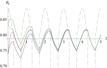
Figure 3: Numerical integration of the driven model corresponding to Example 1, showing the convergence of $\theta_{\mathrm{e}}(t)$ to the limit cycle. The four initial conditions correspond to pairing two different values of $\theta_{\mathrm{e}}$ with two of $\theta_{\mathrm{i}}$. The dashed line represents the temperature equivalent driving $\left[q_{\mathrm{e}}+f(t)\right]^{1/4}$.

If we want to observe the evolution of $\theta_{\mathrm{e}}$ and $\theta_{\mathrm{i}}$ simultaneously, a three-dimensional plot is necessary. However, the plotting of several integral curves in the same graph makes it confusing, so we choose to plot only one, namely, the curve with initial conditions at the fixed point. This plot is displayed in Fig. 4. Notice that the amplitude of the oscillation is sufficiently small for the evolution to stay in a small neighborhood of the sink of the averaged equations, where the linear equations (15) are good approximations (compare the amplitude with the ranges displayed in Fig. 1). The limit cycle can be mentally visualized in this three-dimensional plot by identifying, for example, the plane $t=5$ with the plane $t=4$. Of course, a three-dimensional plot in cylindrical coordinates such that $t$ were the angular coordinate and the temperature planes were orthogonal to it would be more suitable for representing the limit cycle, but that plot would not provide a clear rendering of the line converging to the limit cycle.

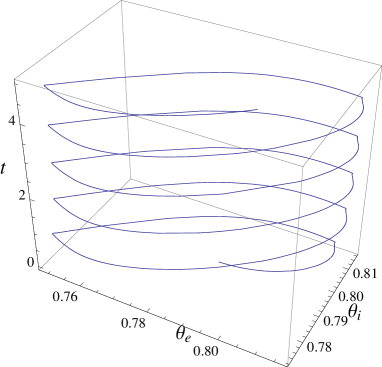
Figure 4: Numerical evolution of the two temperatures of the driven model corresponding to Example 1.

Like in the one-node model [11], one can derive a reasonable approximation of the limit cycle from Eqs. (20) or (21). Since the magnitude of the eigenvalues of $J$ is not small (they are $\{-10.74,-1.024\}$), it is more efficient to use the integral expression (20), because the decrease of the integrand with $\tau$ allows us to compute the integral to a good accuracy by restricting it to a few periods of $f$.

It is interesting to explore what happens for other values of the parameters, especially, for increasing magnitudes of the driving $f$ which could compromise the convergence of the perturbation series. According to Eq. (12) and on account of the proportionality between $q_{\mathrm{a}}$ and $q_{\mathrm{s}}$ (for fixed albedo), $f$ is proportional to $q_{\mathrm{s}}$, that is to say, the driving heat oscillation is proportional to the solar constant. This constant would be larger if we considered a satellite orbiting an inner solar system planet, for example. We have carried out numerical integrations with the values of $q_{\mathrm{s}}$, $q_{\mathrm{a}}$ and $q_{\mathrm{p}}$ (all proportional to the solar constant) increased by a given factor. Nothing remarkable happens with a factor as large as one hundred. However, a factor of about one hundred ninety seems to provoke an instability. For factors larger than 250, the periodic limit-cycle behavior seems to become quasi-periodic, and it even seems to become chaotic for larger factors. We have not studied the transition to chaos in any detail, because such large values of the heat inputs are far from being realistic.

3 Many-node model of a spacecraft

Let us now consider a general many-node thermal model of a spacecraft (it could be a satellite, in particular). The energy balance equations are [6]

$$C_{i}\,\dot{T_{i}}=\dot{Q}_{i}(t)+\sum_{j=1}^{N}{}^{{}^{\prime}}\left[K_{ij}(T_{j}-T_{i})+R_{ij}(T_{j}^{4}-T_{i}^{4})\right]-R_{i}\,{T_{i}}^{4},\quad i=1,\ldots,N,$$ (23)

where $N$ is the number of nodes, and the prime in the sum symbol means that the value $j=i$, namely, the self-coupling, is omitted. $\dot{Q}_{i}(t)$ contains the total heat input to the $i$-node from outside of the spacecraft and from its internal heat dissipation (if there is any). The conductive and radiative couplings are denoted $K$ and $R$, respectively. The couplings between two arbitrary nodes $i$ and $j$ satisfy $K_{ij}=K_{ji}$ and $R_{ij}=R_{ji}\,$. The $i$-node coefficient of radiation to the environment is given by $R_{i}=A_{i}\varepsilon_{i}\sigma$, where $A_{i}$ denotes the outside looking area and $\varepsilon_{i}$ denotes the emissivity. Eqs. (23) basically coincide with the ones implemented in commercial software packages, for example, ESATAN^TM [22].

Like in the two-node case, our first step is to assume in Eqs. (23) that the $\dot{Q}_{i}$ are constant, by replacing the functions $\dot{Q}_{i}(t)$ with their averages. The steady state temperatures are the roots of a system of $N$ algebraic equations of fourth degree. Systems of algebraic equations are notably more difficult to solve than single algebraic equations, but some general facts about them are known. For example, the number of complex roots of a systems of $N$ fourth-degree algebraic equations is $4^{N}$, generically speaking. However, we are only interested in the roots with real and positive $T_{i},\;i=1,\ldots,N$. The problem of finding the physical steady state for the two-node model of Sect. 2 is solved in Sects. 2.1 and 2.2, where we show that, indeed, there is only one root in the positive quadrant and it corresponds to an asymptotically stable state. We now deal with the general problem and prove that there is one and only one asymptotically stable state in the positive orthant.

3.1 Averaged equations: their stable steady state

Let us recall the results for the two-node steady state in Sect. 2.1. The total number of complex roots of the two algebraic equations is indeed $4^{2}=16$. However, to conclude that there are 4 real roots of which only one is in the positive quadrant, we need to reduce the two equations to a single fourth-degree equation and apply Descartes’s rule of signs to it. Unfortunately, this is a very specific procedure tailored to those two algebraic equations. In fact, the general two-node model given by Eqs. (23) with $N=2$ and constant $\dot{Q}_{i},\;i=1,2,$ gives rise to two fourth-degree algebraic equations that do not lend themselves to be reduced to a single fourth-degree algebraic equation. Nonetheless, one can reduce the two equations to a single sixteenth-degree equation; but its analysis is inconclusive, whether we use Descartes’s rule of signs or other standard methods of determining the number of real roots of an algebraic equation [15].

Instead of attempting to find the zeros of the ODE’s vector field directly by solving algebraic equations, we can resort to an indirect method, namely, to a topological method. For a vector field and a closed curve in the plane, one can introduce the Poincaré index of the curve with respect to the vector field, which is the number of turns that the vector makes when a point goes along the curve and returns to its original position [18, 24]. The Poincaré index of a curve is a topological invariant, for it only depends on the singularities (zeros) of the vector field enclosed by the curve. In particular, when the curve encloses no singularities, the index vanishes. Therefore, a non-vanishing index proves the existence of a singularity in the given region. In particular, we can take as test region the positive quadrant: to convert it into a finite region, we can bound it with a curve such that the distance of every point on it to the origin is sufficiently large for the vector field to adopt its asymptotic form, with only its highest degree terms. For the general two-node model, we can then find, in particular, the expression of the vector field on the boundary of a large square with a vertex on the origin and two sides on the positive coordinate semi-axes, and then check that the vector always points inwards. This shows that the index in the square is $+1$, which proves the existence of, at least, one steady state with real and positive $T_{1}$ and $T_{2}$.

To complete the argument, we need to determine the index of the possible steady states. First, let us study their stability. The Jacobian matrix at the point $(T_{1},T_{2})$ is

$$J=\left(\begin{array}[]{cc}[-K_{12}-4(R_{12}+R_{1})T_{1}^{3}]/C_{1}&(K_{12}+4R_{12}\,T_{2}^{3})/C_{1}\\ \left(K_{12}+4R_{12}\,T_{1}^{3}\right)/C_{2}&\left[-K_{12}-4(R_{12}+R_{2})T_{2}^{3}\right]/C_{2}\end{array}\right).$$ (24)

When $R_{2}=0$, its eigenvalues are real and negative (provided that $T_{1},T_{2}>0$), as proved in Sect. 2.2. The proof holds when $R_{2}\neq 0$, so that any fixed point in the physical region must be a sink and, specifically, a node. Now, we can combine this result with the available topological information: since the Poincaré index of a sink is easily seen to be $+1$ [18, 24] and the index is additive, there can only be one sink (in the physical region).

The preceding analysis of the general two-node model can be extended to higher dimensions, for the two-dimensional notion of the index of a curve with respect to a vector field can be generalized to higher dimensions [24], giving rise to the Poincaré-Hopf theorem [25]. Furthermore, the negativity of the eigenvalues of the Jacobian matrix also holds in higher dimensions. However, the proof is not as simple as in the case $N=2$. Indeed, in the general case, we need to introduce some notions of the theory of matrices and then prove a preliminary property of the Jacobian matrix (stated below as a lemma).

The $N$-node equations Jacobian matrix elements are given by:

$$J_{ij} = C_{i}^{-1}\left(K_{ij}+4R_{ij}T_{j}^{3}\right),\quad\mathrm{if}\;i\neq j,$$ (25)

$$J_{ii} = C_{i}^{-1}\left[-\sum_{j=1}^{N}{}^{{}^{\prime}}\left(K_{ij}+4R_{ij}T_{i}^{3}\right)-4R_{i}\,{T_{i}}^{3}\right].$$ (26)

This matrix has positive off-diagonal and negative diagonal elements (if the temperatures are positive). This property can be expressed by saying that $-J$ is a $Z$-matrix [26]. Furthermore, we can prove that it is also a nonsingular $M$-matrix, namely, a $Z$-matrix such that its inverse is non-negative. The condition that its inverse be non-negative is, in fact, just one among a number of equivalent conditions that turn a $Z$-matrix into a nonsingular $M$-matrix: Ref. [26] lists fifty different conditions! In our case, it is convenient to apply the conditions of semipositivity (related to the conditions of diagonal dominance, see Ref. [26]). Thus, we state:
Lemma: The opposite of the Jacobian matrix of Eqs. (23) is a nonsingular $M$-matrix.
Proof: Instead of applying the semipositivity conditions to $-J$, we apply them to its transpose, which is equivalent, since a matrix and its transpose are simultaneously nonsingular $M$-matrices. A matrix is semipositive if there exists a strictly positive vector that stays strictly positive when multiplied by the matrix. Let $v=(C_{1},\ldots,C_{N})$, so

$$\left[-J^{t}\cdot v\right]_{i} = -\sum_{j=1}^{N}{}^{{}^{\prime}}J_{ji}\,C_{j}-J_{ii}\,C_{i}=-\sum_{j=1}^{N}{}^{{}^{\prime}}\left(K_{ji}+4R_{ji}{T_{i}}^{3}\right)+$$ (27)

$$+\sum_{j=1}^{N}{}^{{}^{\prime}}\left(K_{ij}+4R_{ij}T_{i}^{3}\right)+4R_{i}\,{T_{i}}^{3}=4R_{i}\,{T_{i}}^{3}\geq 0.$$

Therefore, the vector $-J^{t}\cdot v$ is strictly positive if no $R_{i}$ vanishes, but it is just positive if some of these coefficients do vanish. Then, the matrix and the vector must fulfill additional conditions [26], which are, in our case:

$$\sum_{j=1}^{i}\left(-J^{t}\right)_{ij}C_{j}>0\,,\quad i=1,\ldots,N.$$

These conditions hold if we choose a node order such that $R_{N}\neq 0$, which is possible, unless $R_{i}=0$ for all $i=1,\ldots,N$. In conclusion, $-J^{t}$ and hence $-J$ are nonsingular $M$-matrices, q.e.d.

Once we know that $-J$ is a nonsingular $M$-matrix, we can use a crucial property of its eigenvalues: their real parts are positive [26]. In fact, an $M$-matrix actually plays the rôle of “a poor man’s positive definite matrix.” In particular, the condition that the eigenvalues of $J$ have negative real parts (in the physical region) is sufficient to affirm the asymptotic stability of any steady state, even if the eigenvalues have non-vanishing imaginary parts. Therefore, any physical steady state has to be a sink. Taking this into account, we can state the following theorem:
Theorem: Eqs. (23) with constant $\dot{Q}_{i},\;i=1,\ldots,N,$ have in the positive orthant a unique steady state that is asymptotically stable.
Proof: We first prove the existence of a steady state in the positive orthant. Using the boundary of a large hypercube drawn from the origin in the directions of positive $T_{i}$ ($i=1,\ldots,N$), it is easy to show that the vector field defined by Eqs. (23) (with constant $\dot{Q}_{i}$) points inwards. Indeed, on the hypercube side $T_{i}=0$, the $i$-component of the vector field is trivially positive, while on the opposite side, $T_{j}<T_{i}$ for each $j\neq i$, making the $i$-component negative for large $T_{i}$. Therefore, one deduces that the Poincaré-Hopf index is non-vanishing and actually is $(-1)^{N}$. Although this non-vanishing index proves the existence of a steady state, it does not prove that it is unique. However, we already know that any physical steady state is a sink, and a sink has Poincaré-Hopf index $(-1)^{N}$. On account of the additivity of the Poincaré-Hopf indices, it follows that the sink in the positive orthant is unique, q.e.d.

Of course, we have only proved local stability. In Subsec. 2.2, we have also established the global stability of the restricted two-node steady state by appealing to some general theorems due to the topological restrictions of two-dimensional flows. Thus, the proof given in Subsec. 2.2 is also valid for the general two-node model. In three or more dimensions, there are no equivalent topological restrictions and the question of global stability is moot. This is natural, given that autonomous systems of three ODE’s can have very complex flows and, in particular, can have chaotic attractors.

Since $J$ is diagonalizable with real eigenvalues in the case of the two-node model, we would like to know if this holds for $N>2$. Let us consider, for example, the three-node model. It gives rise to a $3\times 3$ Jacobian matrix and, hence, to a third-degree algebraic equation for the eigenvalues. If the discriminant of this equation were positive, then its roots would be three different real numbers [14] and, therefore, the Jacobian matrix would be diagonalizable (like in the case of the two-node model). Unfortunately, the discriminant of a third-degree algebraic equation is a complicated fourth-degree polynomial in its coefficients. Furthermore, the coefficients of the eigenvalue equation for a $3\times 3$ matrix are complicated polynomials in the matrix elements. As a polynomial in these matrix elements, the discriminant has sixth degree and consists of 144 monomials with positive and negative signs. Thus, it is very difficult to decide on the overall sign of this discriminant, despite that the Jacobian matrix elements have definite signs.

The question of whether or not the Jacobian matrix is diagonalizable with real eigenvalues can be considered from a different point of view. Given the expressions of the Jacobian matrix elements (25) and (26), the matrix is simplified somewhat by multiplying it on the left by the diagonal matrix $D=\mathrm{diag}(C_{1},\ldots,C_{n})$, which removes the factors $C_{i}^{-1}$. If $D\cdot J$ were symmetric, $D^{1/2}\cdot J\cdot D^{-1/2}$ would be symmetric as well, as is easily proved. Therefore, $J$ would be similar to a symmetric matrix and hence would be diagonalizable with real eigenvalues. The matrix elements of the symmetric and antisymmetric parts of $D\cdot J$ are, respectively, $K_{ij}+2R_{ij}\left(T_{i}^{3}+T_{j}^{3}\right)$ and $2R_{ij}\left(T_{i}^{3}-T_{j}^{3}\right)$ (for $i\neq j$). If the latter matrix element is of small magnitude with respect to the former for each pair of nodes, then $D\cdot J$ is nearly symmetric and $J$ is likely to be diagonalizable with real eigenvalues. This can be deduced by considering that the eigenvalues of a matrix and their respective eigenvectors vary continuously with the matrix elements and that the eigenvectors of a symmetric matrix are orthogonal. Therefore, if a variation of the elements of a symmetric matrix is to turn two real eigenvalues into a couple of complex conjugate eigenvalues, then it must have sufficient magnitude to change the directions of the respective eigenvectors so much that they coincide.

It is pertinent here to comment that the procedures used in the literature for linearizing the $N$-node ODE’s (23) amount to an ad-hoc symmetrization of the matrix $D\cdot J$, either by assuming that the steady-state node temperatures are approximately uniform [6] or, more accurately, by assuming that they fulfill $\left|T_{i}-T_{j}\right|\ll(T_{i}+T_{j})/2$, for each pair of nodes $ij$ such that $R_{ij}\neq 0$ [10].

3.2 Slowest variable and convergence to the steady state

We have proved above that the eigenvalues of the Jacobian matrix $J$ have negative real parts and, furthermore, we have argued that they are likely real. In this section, we focus on the eigenvalue of smallest absolute value, corresponding to the slowest thermal mode, and we prove that, indeed, it is real. The slowest mode is especially important because it eventually determines the dynamics and the convergence to the steady state. For the proof, we appeal to Perron’s theorem for positive matrices: a positive matrix has a unique real and positive eigenvalue with a strictly positive eigenvector and, furthermore, that eigenvalue has maximal modulus among all the eigenvalues [26]. Since the inverse of $-J$ is non-negative, it is a good candidate for Perron’s theorem: if it is actually strictly positive, its maximal modulus eigenvalue corresponds to the minimal modulus eigenvalue of $J$.

However, it is not easy to find whether or not the inverse of $-J$ is strictly positive. We can apply instead the following theorem: an irreducible $Z$-matrix is a nonsingular $M$-matrix if and only if its inverse is strictly positive [26]. A matrix is said to be reducible if it can be put in a block upper-triangular form by a simultaneous permutation of its files and columns. Therefore, we only need to show that $J$ is irreducible. It would certainly be so if $K_{ij}$ or $R_{ij}$ did not vanish for any pair of indices (except when $i=j$); but some (or many) of the conductive and radiative couplings are expected to vanish simultaneously. Let us assume that we can relabel the nodes and hence permute simultaneously the files and columns of $J$ to make it block upper-triangular. Given that an element $J_{ij}$ only vanishes if both $K_{ij}$ and $R_{ij}$ vanish, according to Eq. (25), both elements $J_{ij}$ and $J_{ji}$ vanish or do not vanish simultaneously. In consequence, an order of nodes that makes $J$ block upper-triangular also makes it block diagonal. A matrix that can be put in a block diagonal form by a simultaneous permutation of its files and columns is said to be completely reducible. However, $J$ is completely reducible if and only if the node model splits into two disconnected node models, which corresponds to modelling two separated spacecrafts.

In conclusion, the matrix $J$ is irreducible for a single spacecraft model and we can apply Perron’s theorem to $(-J)^{-1}$: the largest eigenvalue of the latter corresponds to the negative eigenvalue of $J$ of smallest magnitude and, therefore, to the slowest variable. Furthermore, the corresponding eigenvector is positive and, actually, the only positive eigenvector. Therefore, the sink is eventually approached either from the zone corresponding to simultaneous temperature increments or from the zone corresponding to simultaneous temperature decrements, as already observed for the two-node models in Sect. 2.3. In other words, the slow mode corresponds to a simultaneous increase or decrease of the (non-uniform) temperature throughout the spacecraft whereas faster modes correspond to temperature increases in one or more parts of the spacecraft that are accompanied by decreases in other parts.

3.3 Driven many-node model

If we assume that the heat inputs $\dot{Q_{i}}(t)$ are periodic, the non-autonomous equations (23) is a generalization of the driven two-node model studied in Sects. 2.4 and 2.5. Thus, we can use the equations in Sect. 2.5, if we replace the $\theta_{i}$ with $T_{i}$ and use the driving term

$$F_{i}(t)=\frac{\dot{Q_{i}}(t)-\langle{\dot{Q_{i}}}\rangle}{C_{i}}\,,\quad i=1,\ldots,N,$$

where $\langle{\dot{Q_{i}}}\rangle$ is the mean value of $\dot{Q_{i}}(t)$ over the period of oscillation. The first order perturbative correction $T_{(1)j}(t)$ to the solution of the averaged equations is the solution of the system of linear ODE’s (15), where $\theta_{(1)j}$ must be substituted by $T_{(1)j}$. The subsequent steps are independent of the dimension. Therefore, the integral expression (20) of the limit cycle holds (after replacing $\theta$ with $T$).

If we use the basis of the eigenvectors of $J$ (assuming that $J$ is diagonalizable), the limit cycle ${T}_{(1)}^{\infty}(t)$ becomes a sum of contributions, each one corresponding to an eigenvector. In particular, if $f$ is the component of $F$ along some eigenvector with an eigenvalue $\l$ that is large compared with the heat-input frequency, the corresponding contribution to ${T}_{(1)}^{\infty}(t)$ is approximately equal to $f(t)/\l$. In a many-node model such that the magnitudes of the $J$-eigenvalues span a long range, surely only a few of the slowest modes make significant contributions to ${T}_{(1)}^{\infty}(t)$. This observation suggests an effective method of computing a numerical approximation of the limit cycle: one is to begin with the contributions of the slowest modes and keep adding modes until the addend becomes negligible with respect to the partial sum.

As regards the full perturbation series $\sum_{i}{T}_{(i)}^{\infty}(t)$, one could be more concerned about its convergence now than in the two-node case, since we cannot affirm that the steady state of the averaged system is globally stable. However, exploratory numerical work carried out for models with few nodes for various values of the parameters suggests that the steady state of the averaged system is globally stable and that the perturbation series has good convergence properties. Of course, these numerical results have heuristic value only.

4 Summary and discussion

This work is devoted to the study of the nonlinear ODE’s employed in spacecraft thermal control, with emphasis on analytic methods. We have first studied a satellite model consisting of two nodes, namely, the satellite’s exterior and interior parts. Comparing the results obtained for this model with the results for the one-node model in Ref. [11], we see that the addition of one node does not give rise to any essentially new features, as long as the heat inputs vary moderately. In fact, with constant heat input and when the thermal coupling between the two nodes is sufficiently strong, as in Example 1 in Subsect. 2.3.2, the two-node model naturally evolves towards the one-node model. This evolution pattern is ascertained by two results: (i) the existence of a globally stable steady state in which the temperatures of the two nodes become almost equal; and (ii) the appearance of a fast dynamical variable, such that the two-node model dynamics converges to a one-node model dynamics before reaching the steady state.

When the coupling between the two nodes is weak, as in Example 2 in Subsect. 2.3.2, there is also a physical steady state and a fast variable, but the heat balance is reached in a more complicated way. The ratio of the inner to the outer node temperatures in the steady state is still close to one, e.g., $T_{\mathrm{i}}/T_{\mathrm{e}}=1.116$ in Example 2, but the ratio between the increments of the respective temperatures, given by the positive eigenvector, can now be considerable: it is $\Delta T_{\mathrm{i}}/\Delta T_{\mathrm{e}}=3.103$ in Example 2. Therefore, the transition to the slow dynamics does not imply that the node temperatures approach each other over the typical time of the fast variable, although they do so over the typical time of the slow variable.

A periodic heat input produces nonlinear driven oscillations of the temperatures, namely, a limit cycle. This can be proved by taking the oscillating heat input as a perturbation and expanding the nonlinear system in series, thus converting it into a set of linear systems. At the first order, the linear equation valid on long times is just the equation of driven overdamped linear oscillations and it has the standard solution. We find that the perturbative series is convergent in a range of amplitudes of the driving heat input that is sufficient for the applications. Moreover, the perturbative series allows one to calculate, order by order, the limit cycle and the convergence of the temperatures to it. We have found numerical evidence of more complex behaviors, probably including quasiperiodicity and chaos, but these behaviors take place for unrealistic amplitudes of the driving heat input.

Most of the above conclusions can be extended to the general $N$-node thermal model of a spacecraft, by employing topological methods and the theory of non-negative matrices. For constant heat input, the general $N$-node model also has an attractive steady state in the physical region and the dynamics converges to a slow variable corresponding to a simultaneous increase or decrease of the (non-uniform) temperature throughout the spacecraft. However, we are unable to prove the global stability of the steady state. In this regard, we must notice that most proofs in the theory of differential equations have local nature and, in fact, global properties can only be proved with powerful mathematical tools. One such tool is the topological index, but it only provides partial information. Another powerful tool is the existence of a Lyapunov function [12, 13]: a global strict Lyapunov function allows one to determine the global stability of a sink. Unfortunately, there are no general methods for finding suitable Lyapunov functions. For ODE’s with physical origin, sometimes it is possible to find a physically motivated Lyapunov function, for example, an energy, entropy, etc. Thus, there could be a physically motivated Lyapunov function for the $N$-node model ODE system, but it is certainly hard to find.

When driven by a periodic heat input, the $N$-node model also becomes a nonlinear oscillator. But one could be more concerned about the range of convergence of the perturbative series for this model than about the series for the two-node model. At any rate, when the dynamics is confined to a neighborhood of the steady state, no high order terms of the perturbative series are needed. The amplitude of the two-node model limit cycle is indeed small and the linear first-order equation suffices; but its steady state is, of course, globally stable anyhow. Regarding $N$-node models, we believe that the relevant values of the parameters do not produce large amplitudes either and that the linear first-order equations may suffice. Notice, however, that those equations do not coincide with previous types of linearization, in which the coefficient matrix of the ODE system is forced to be related to a symmetric matrix by defining radiative conductances that depend on somewhat arbitrary temperatures (as in Refs. [6, 7, 10]). In contrast, the linear equations are not equivalent to the equations of a model with only conductive thermal couplings and the actual Jacobian matrix of the ODE system is not related to any symmetric matrix.

Regarding the practical use of $N$-node thermal models, we must notice that the diagonalization of the Jacobian matrix at the steady state usually yields (negative) eigenvalues of very different magnitude, like in our two examples of a two-node model. The fast variables indicate the regions of the spacecraft where the heat inputs and outputs quickly balance, establishing a dynamical balance long before the steady state is reached. The last and longest stage of this dynamical balance corresponds to the slowest variable, with definite ratios of the temperature increments. We believe that it is interesting to distinguish the response of the different modes in regard to spacecraft thermal control. Standard software packages for spacecraft thermal analysis do not regard this aspect of the solution of the equations.

Besides, our results have some bearing on an interesting problem of lumped-parameter models, namely, the problem of node condensation: a model is normally constructed heuristically and it can be useful to reduce its number of nodes while preserving the required performance of its design. In a spacecraft thermal model, if a couple of nodes $ij$ are such that their steady temperatures fulfill $T_{i}\simeq T_{j}$ and $\Delta T_{i}\simeq\Delta T_{j}$, it may be advisable to replace them by a single node, because that will not result in a loss of accuracy in the description of the temperature distribution. According to our results, this type of condensation can be achieved at no great computational cost: one only needs to compute the steady temperatures and then the positive eigenvector of the corresponding Jacobian matrix.

The determination of a spacecraft’s thermal modes and their use for node condensation are beyond the scope of current thermal software packages. Therefore, the analytic approach proposed here can be a useful complement to the analysis that is normally carried out with those software packages.

Acknowledgments

I thank Angel Sanz-Andrés for conversations.

References

- [1] F. Kreith, Radiation Heat Transfer for Spacecraft and Solar Power Plant Design. Intnal. Textbook Co., Scranton, Penn. (1962)
- [2] C.A. Wingate, Spacecraft Thermal Control. In: Fundamentals of Space Systems, V.L. Pisacane and R.G. Moore (eds.), Oxford Univ. Press (1994)
- [3] R.A. Henderson, Thermal control of spacecraft. In: Spacecraft Systems Engineering, Second Edition, P. Fortescue and J. Stark (eds.), Wiley, Chichester (1995)
- [4] G. Gilmore (ed.), Spacecraft Thermal Control Handbook. The Aerospace Press, El Segundo (2002)
- [5] C.J. Savage, Thermal control of spacecraft. In: Spacecraft Systems Engineering, Third Edition, P. Fortescue, J. Stark and G. Swinerd (eds.), Wiley, Chichester (2003)
- [6] K. Oshima and Y. Oshima, An analytical approach to the thermal design of spacecrafts. Rep. No. 419, Inst. of Space and Aeronautical Science of Tokio (1968)
- [7] C. Arduini, G. Laneve and S. Folco, Linearized techniques for solving the inverse problem in the satellite thermal control. Acta Astronautica 43, 473–479 (1998)
- [8] J.-R. Tsai, Overview of satellite thermal analytical model. Journal of Spacecraft and Rockets, 41, 120–125 (2004)
- [9] M.A. Gadalla, Prediction of temperature variation in a rotating spacecraft in space environment. Applied Thermal Engineering 25, 2379–2397 (2005)
- [10] I. Pérez-Grande, A. Sanz-Andrés, C. Guerra and G. Alonso, Analytical study of the thermal behaviour and stability of a small satellite. Applied Thermal Engineering 29, 2567–2573 (2009)
- [11] J. Gaite, A. Sanz-Andrés and I. Pérez-Grande, Nonlinear analysis of a simple model of temperature evolution in a satellite. Nonlinear Dynamics 58, 405–415 (2009)
- [12] J. Guckenheimer and P. Holmes, Nonlinear Oscillations, Dynamical Systems, and Bifurcations of Vector Fields. Springer (1983)
- [13] P.G. Drazin, Nonlinear Systems. Cambridge texts in applied mathematics, Cambridge U.P. (1992)
- [14] J.-P. Tignol, Galois’ Theory of Algebraic Equations. World Scientific, Singapore (2001)
- [15] J. Hymers, A treatise on the theory of algebraical equations. Cambridge (1858)
- [16] H.B. Callen, Thermodynamics and an Introduction to Thermostatistics. Second Edition, Wiley (1985)
- [17] A.H. Nayfeh and D.T. Mook, Nonlinear Oscillations. Wiley Classics Library (1979)
- [18] A.A. Andronov, A.A. Vitt and S.E. Khaikin, Theory of Oscillators. Dover, N.Y. (1987)
- [19] W. Hurewicz, Lectures on Ordinary Differential Equations. Technology Press, MIT (1958)
- [20] A.H. Nayfeh, Perturbation Methods. Wiley Classics Library (2000)
- [21] M.W. Hirsch and S. Smale, Differential Equations, Dynamical Systems, and Linear Algebra. Pure and Applied Mathematics, Academic Press, N.Y. (1974)
- [22] ESATAN-TMS Thermal Engineering Manual. Prepared by ITP Engines UK Ltd., Whetstone, Leicester, UK (2009)
- [23] I. Shafarevich, Basic algebraic geometry. Springer (1974)
- [24] V.I. Arnold, Ordinary Differential Equations. MIT Press, Cambridge (1973)
- [25] M. Hazewinkel, Poincaré-Hopf theorem. In: The Encyclopaedia of Mathematics, (Springer, 2002), available online at http://eom.springer.de/p/p110160.htm
- [26] A. Berman and R.J. Plemmons, Nonnegative Matrices in the Mathematical Sciences. Classics in Applied Mathematics, vol. 9, SIAM (1994)