Estimating Effects and Making Predictions from Genome-Wide Marker Data

Abstract

In genome-wide association studies (GWAS), hundreds of thousands of genetic markers (SNPs) are tested for association with a trait or phenotype. Reported effects tend to be larger in magnitude than the true effects of these markers, the so-called “winner’s curse.” We argue that the classical definition of unbiasedness is not useful in this context and propose to use a different definition of unbiasedness that is a property of the estimator we advocate. We suggest an integrated approach to the estimation of the SNP effects and to the prediction of trait values, treating SNP effects as random instead of fixed effects. Statistical methods traditionally used in the prediction of trait values in the genetics of livestock, which predates the availability of SNP data, can be applied to analysis of GWAS, giving better estimates of the SNP effects and predictions of phenotypic and genetic values in individuals.

, , and

1 Introduction

The rules for the genetic inheritance of traits, discovered by Mendel, are most obvious for traits controlled by a single gene, for example, individuals who carry two defective variants in the gene CFTR develop cystic fibrosis. However, most of the traits that are of importance in medicine, agriculture and evolution are influenced by many genes and by nongenetic or “environmental” factors. For example,height in humans involves many physiological processes and many genes but is also influenced by nongenetic factors such as nutrition and health care. These traits are called quantitative or complex traits and include common genetic diseases such as heart disease, breast cancer, diabetes and psychiatric disorders.

Until recently few of the genes which harbor variants for complex genetic traits had been identified. The availability of genome-wide panels of densely spaced, genetic markers has led to a revolution in the study of the genetics of complex traits. These genetic markers are single nucleotide polymorphisms (SNPs) which are positions in the DNA sequence where the nucleotides can vary (e.g., G or T). Individuals carry pairs of homologous chromosomes and so have one of three genotypes at a G/T SNP—GG, GT or TT. Assays are now available that determine the genotype of an individual at 100,000 to over 1 million SNPs spread over all of the chromosomes of the species.

SNPs usually have no direct effect on a trait under study. However, any polymorphism that does affect the trait will be located on a chromosome close to one or more of the genotyped SNPs because the genotyped SNPs are chosen to cover all chromosomes in, at least, moderate density. Polymorphisms that are located close to each other on a chromosome can occur together more often than expected by chance, so that they are correlated or in linkage disequilibrium (LD). Thus, for every polymorphism that affects a trait, there is likely to be a SNP nearby that is in LD with the causal polymorphism and hence correlated or associated with the trait. Since the SNPs cover the whole genome, experiments that test for association between a trait and a panel of SNPs that cover the whole genome are called genome wide association studies (GWAS). GWAS have discovered numerous SNPs that are associated with, for example, complex diseases such as Crohn’s disease and type II diabetes 1 , 2 . Typically there are multiple SNPs associated with a complex trait, each one with a small effect, or a small increase in the risk of a particular disease.

One purpose of a GWAS might be to find the genes and polymorphisms that affect the trait. Hopefully this will elucidate the biology of the trait and, in human medicine, may lead to new therapeutics. In this case we would like to have unbiased and accurate estimates of the effects of SNPs on the trait on which to base further experimentation. Another use of the GWAS is to use the SNPs to predict the phenotypic or genetic value of individuals. For example, in agriculture it would be very useful to predict the genetic merit of bulls for milk production using DNA markers such as SNPs, because it is not possible to observe the phenotype (milk yield) in bulls and, even if it were possible, it is the genetic value of the bull that will be passed on to his descendants. Also, if we could predict the risk of a specific disease in individuals based on DNA markers this would be useful in diagnosis, treatment, prognosis and prevention. The DNA markers cannot predict the environmental effect on a complex trait, only the genetic value for that trait. Hence, the genetic value and phenotypic value predicted from DNA markers are the same. The question to be considered is as follows: how can this prediction be made as accurately as possible?

Statistical analysis of GWAS may test hypotheses (e.g., there are no SNPs associated with this trait) or estimate the effect of a SNP on the trait (e.g., how much does this SNP affect the probability that a person will develop diabetes). In such estimation problems the tendency has been to treat the effect of a SNP as a fixed effect and use estimators that are classically unbiased, at least approximately, such as the maximum likelihood estimate of the relative risk of disease. However, in GWAS hundreds of thousands of SNPs are tested, but frequently the estimated effects are reported only for the significant markers, for example, 1 . Under these conditions, it has been known for some time that the reported effects tend to be larger in magnitude than the true effects of these markers. This effect is known as the “Beavis effect” in agricultural genetics 3 , 4 as cited in 5 , and has been described as a form of the “winner’s curse” 6 . Methods to correct for this bias have been published 3 , 6 , 7 , 8 , 9 , 10 , 11 , 12 , 13 , 14 , 15 . We argue that the classical definition of unbiasedness is not useful in this context and propose to use a different definition of unbiasedness that is a property of the estimator we advocate in this paper. This definition of unbiasedness has a strong theoretical underpinning 16 , 17 and has traditionally been used and applied in agricultural genetics 16 , 17 , 18 , 19 , 20 .

Another motivation for the statistical analysis of GWAS might be to use the SNP genotypes to predict the value of a trait that has not yet been observed, for example, to predict the future risk of a disease for an individual person. This has parallels to predicting a person’s risk of disease based on their family history of that disease. Generally, when such prediction is carried out, the variable being predicted is regarded as a random variable. Then the prediction might use the multiple regression of the trait or phenotypic value on the SNP genotypes. If the biased estimates of the SNP effects described in the previous paragraph are used in this regression equation, then the predictions will exaggerate the variation in risk between individuals.

In this paper we suggest an integrated approach to the estimation of the SNP effects and to the prediction of trait values that overcomes the bias in both. It relies on treating the SNP effects as random, instead of fixed, effects. There is a well-established statistical tradition of prediction of trait values in the genetics of livestock and we introduce this methodology in the first section of the paper. This methodology predates the availability of SNP data and uses the equivalent of family history, that is, phenotypic values on relatives of the individual whose phenotype we wish to predict. Then we show how this approach can be applied to analysis of GWAS giving better estimates of the SNP effects and predictions of phenotypic and genetic values in individuals. In fact, there is equivalence between models of genetic value based on SNPs and one based on relationships between individuals, and this equivalence is explained. We then give results from the analysis of GWAS. Finally we discuss how this approach will cope with future developments such as whole genome resequencing.

2 Prediction

2.1 Prediction of Phenotypic Values from Pedigree Data

To illustrate our approach, we will describe a specific example and then generalize. Imagine that we have data consisting of the milk yields of cows that belong to a number of half-sib families (all cows within a half sib family have the same sire) and we wish to predict the milk yields of future cows within any of these half-sib families. The milk yields of cows within a family are correlated and we can use this to predict the yield of a future cow from the same family ($y_{\mathrm{future}})$. In general, the predictor of a random variable that has the lowest mean square error of prediction is the conditional mean given the data available for prediction 16 , 17 , 19 , 21 . This predictor is called the best predictor 17 , 20 . In the case of predicting the milk yield of a future cow conditional on the milk yields observed on existing cows in the same family ($\mathbf{y}_{\mathrm{existing}}$), the best predictor ($\hat{y}$) is the expected value of the milk yield of a future cow. That is,

$$\hat{y}=\mathrm{E}(y_{\mathrm{future}}|\mathbf{y}_{\mathrm{existing}}).$$

If the $y$ follows a multivariate normal distribution, then E($y_{\mathrm{future}}|\mathbf{y}_{\mathrm{existing}})$ is the linear regression of$y_{\mathrm{future}}$ on $\mathbf{y}_{\mathrm{existing}}$. If

$$V(\matrix{y_{\mathrm{future}}&\mathbf{y}_{\mathrm{existing}}})=\mathbf{V}=\left[\matrix{{V}_{\mathrm{future}}&\mathbf{v}\cr\mathbf{v}^{\prime}&\mathbf{V}_{\mathrm{existing}}}\right],$$

then $\hat{y}=\mathbf{v}^{\prime}\mathbf{V}_{\mathrm{existing}}^{-1}y_{\mathrm{existing}}$. Since all cows within a family share the same relationship with each other, the diagonal elements of $\mathbf{V}$ are all equal, as are the off-diagonal elements. That is, $\mathbf{V}=\mathbf{I}\sigma_{e}^{2}+\mathbf{J}\sigma_{s}^{2}$, where $\mathbf{I}$ is the identity matrix, $\mathbf{J}$ is a matrix of all ones, $\sigma_{e}^{2}+\sigma_{s}^{2}$ is the variance of milk yield and $\sigma_{s}^{2}$ is the covariance between the milk yields of cows from the same family.

An equivalent model, generalized to $n$ milk yield records from $f$ sire families, that leads to the same prediction is as follows:

$$\mathbf{y}=\mathbf{Zs}+\mathbf{e},$$

where

• $\mathbf{y}$ is an $n\times 1$ vector of milk yields for all cows over $f$ families,

• $\mathbf{Z}$ is an $n\times f$ matrix that allocates cows to families,

• $\mathbf{s}$ is an $f\times 1$ vector of sire effects $\sim\mathrm{N}(0,\mathbf{I}\sigma_{s}^{2})$,

• $\mathbf{e}$ is an $n\times 1$ vector of independent errors or environmental effects $\sim\mathrm{N}(0,\mathbf{I}\sigma_{e}^{2})$.

The best predictor of $\mathbf{s}$ is

$$\hat{\mathbf{s}}=\mathbf{Z}^{\prime}(\mathbf{ZZ}^{\prime}\sigma_{s}^{2}+\mathbf{I}\sigma_{e}^{2})^{-1}\mathbf{y}$$

and the best predictor of $y$ for a future cow is

$$\hat{y}=\mathbf{z}_{\mathrm{future}}^{\prime}\hat{\mathbf{s}},$$

where $\mathbf{z}_{\mathrm{future}}$ is a vector of zeros with a single one, to indicate to which family the future cow belongs.

For the $i$th sire, $\hat{s}_{i}$ can also be written as $y_{i}n_{i}/(n_{i}+\lambda))$, where $y_{i}$ is the mean of $y$ for the $n_{i}$ cows in the $i$th family and $\lambda=\sigma_{e}^{2}/\sigma_{s}^{2}$. This is a linear model and $\hat{s}_{i}$ is an estimate of the sire effect ($s_{i}$), but it is not the conventional estimate derived from treating sire effects as fixed effects which would be $\tilde{s}_{i}=y_{i}$. Estimates such as $\tilde{s}$ are unbiased in the traditional sense, that is, they have the property

$$\mathrm{E}(\tilde{s}|s)=s.$$ (1)

By contrast, $\hat{s}$ is not unbiased in the sense of (1) because it is a “shrunk” estimate.

In what respect is $\hat{y}$ the best predictor of $y?$ It has the minimum prediction error variance $\operatorname{var}(\hat{y}-y)$. Similarly, $\hat{s}$ has the minimum $\operatorname{var}(\hat{s}-s)$. $\hat{s}$ also has the property 16 , 19 , 20 , 21

$$\mathrm{E}(s|\hat{s})=\hat{s}.$$ (2)

Equation (2) defines a type of unbiasedness which is only meaningful when $s$ is regarded as a random effect. It can be stated as follows: If, on the basis of this analysis, one selects a group of sires whose average value of $\hat{s}$ is $k$ and one produces one more daughter from each of these sires, then the expected mean milk yield of these future daughters is $k$.

In practice, the statistical model for milk yields would include some fixed effects ($\mathbf{c}$), as well as the random effect of sire, in a mixed model. That is,

$$\mathbf{y}=\mathbf{Xc}+\mathbf{Zs}+\mathbf{e}.$$

Also, the sires might be related and so $\mathbf{s}\sim\mathrm{N}(0,\mathrm{A}_{s}\sigma_{s}^{2})$, where $\mathbf{A}_{s}$ is the numerator relationship matrix (which is twice the kinship matrix 18 ) derived from the pedigree of the animals. The solutions from the equations

$$\left[\matrix{\mathbf{X^{\prime}X}&\mathbf{X^{\prime}Z}\cr\mathbf{Z^{\prime}X}&\mathbf{Z^{\prime}Z+A}_{{s}}^{-1}\lambda}\right]^{-1}\left[\matrix{\mathbf{X^{\prime}y}\cr\mathbf{Z^{\prime}y}}\right]$$

are Best Linear Unbiased Estimates (BLUEs) of the fixed effects and Best Linear Unbiased Predictors (BLUPs) of the random effects 16 , 20 . In fact, we can model the observed phenotypes in terms of the genetic value of each individual ($\mathbf{a}$) as

$$\mathbf{y}=\mathbf{Xc}+\mathbf{Ta}+\mathbf{e},$$

where $\mathbf{a}$ is a vector of additive genetic values$\sim$$\mathrm{N}(0,\mathbf{A}\sigma_{{a}}^{2})$ where $\mathbf{A}$ is a numerator relationship matrix like $\mathbf{A}_{s}$ but recording the relationships between individuals, including the relationships caused by cows with the same sire. The BLUP equations become

$$\left[\matrix{\mathbf{X^{\prime}T}&\mathbf{X^{\prime}T}\cr\mathbf{T^{\prime}X}&\mathbf{T^{\prime}T}+\mathbf{A}^{-1}\frac{\sigma_{e}^{2}}{\sigma_{a}^{2}}}\right]^{-1}\left[\matrix{\mathbf{X^{\prime}y}\cr\mathbf{T^{\prime}y}}\right].$$

In livestock genetics this is known as an “animal model” because the genetic value of each individual is explicitly included in the model together with the relationship between all animals. This model has also been used in evolutionary genetic studies 22 and in QTL linkage mapping studies in human pedigrees 23 . For linear mixed models containing fixed and random effects, property (2) holds when the estimates are obtained using BLUP, provided the effects are normally distributed with known variances 16 , 17 .

2.2 Prediction of Phenotype from SNP Genotypes and Estimation of SNP Effects

In the analysis of a GWAS we would like to both predict the phenotype of individuals with observed genotypes but no observed phenotype and to estimate the effects of the SNPs. Both these objectives can be achieved in a consistent manner if we treat the SNP effects as random, just as we did the sire effects above. The structure of the data is typically as follows. There is a reference or discovery sample of individuals who have been typed for the SNPs and recorded for the phenotype. From this data a prediction equation is derived that predicts phenotypes from SNP genotypes. This prediction equation is then used on a validation sample and the accuracy of prediction that we wish to maximize is the accuracy of predicting phenotypes in this sample.

What properties would an ideal predictor have and what measure of accuracy should be maximized? We propose that the ideal predictor is the expectation of the phenotype conditional on the SNP genotypes. That is, if the phenotype is $y$, the predictor $\hat{y}$ should be

$$\hat{y}=E(y|\mathrm{SNP}\mbox{ genotypes}).$$

This property has many advantages. It maximizes the correlation between $y$ and $\hat{y}$, minimizes the error mean square and results in a regression of $y$ on $\hat{y},\beta(y,\hat{y})=1$ 16 , 20 . Consistent with this approach, we would estimate the SNP effects ($b$) such that

$$\hat{b}=E(b|\mbox{ data on phenotypes and genotypes}).$$

This estimator is also unbiased in the sense of (2) and has the same properties as listed for $\hat{y}$ above.

2.3 Comparison with Traditional Fixed Effect Estimators

Usually the effects of SNPs in GWAS have been estimated by methods that are unbiased in the traditional sense of having property (1). To demonstrate that an estimator is unbiased in this sense, we would test the same marker in numerous replicate experiments and average the estimates over these replicates. The simple least squares estimate of $b$ is unbiased in this sense. (We use “least squares” throughout as an example of an estimation procedure that does not shrink estimates. Other estimation procedures, for example, maximum likelihood to estimate odds ratios using logistic regression, fall in the same category.) However, this unbiased property is lost if we only average the estimates over the replicates in which the marker effect was declared “significant” according to some arbitrary threshold of the test statistic. This effect is illustrated in Figure 1 where a SNP with effect 1.0 and standard error 1.0 is declared significant only if the estimated effect $\hat{b}$ exceeds 2.0. In those significant replicates, the mean estimate of $b$ is $\sim$2.5. Methods such as 6 , 8 , 24 attempt to correct for this bias so that the average of $\hat{b}$ over the significant replicates is $b$.

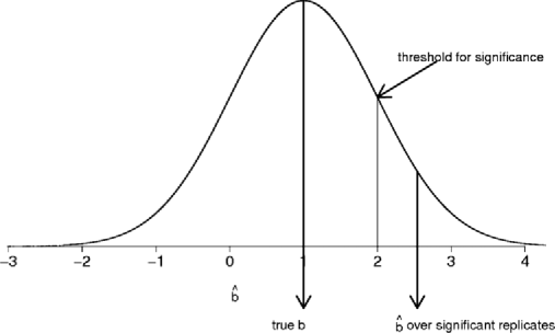
Figure 1: The mean value of $\hat{b}$ ($\sim 2.5$) from significant replicates when $b=1.0$, the threshold for significance is 2.0 and the SE of $\hat{b}$ is 1.0.

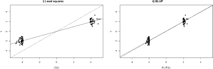
Figure 2: Comparison of conventional least squares (LS) estimates (i) and BLUP estimates (ii) of the effects of SNPs. The true SNP effects were simulated $\sim$N(0, 0.5) and estimated with sampling $\mathrm{error}\sim\mathrm{N}(0,0.5)$. The SNPs with the largest magnitude of effect are plotted ($|\operatorname{LS}(b)|>4$). The BLUP estimates are unbiased, while the least squares estimates overestimated the magnitude of the largest effects. The dashed line shows $y=x$ and the solid line is the regression of $b$ on the $\operatorname{LS}(b)$ or $\operatorname{BLUP}(b)$. BLUP estimates are unbiased irrespective of the threshold chosen for selection.

Conversely, we recommend estimators of SNP effects which are unbiased in the sense of (2) rather than the usual estimators which are unbiased in the sense of (1). Which type of unbiased estimator do we want? We argue that unbiasedness of type (2) is more useful. Estimators of type (2) maximize the correlation between $b$ and $\hat{b}$, minimize the error mean square and result in a regression of $b$ on $\hat{b},\beta(b,\hat{b})=1$. Estimators of type (1) do not have these properties because $\operatorname{var}(\hat{b})>\operatorname{Cov}(b,\hat{b})$, that is, the variance of the predictor is larger than its covariance with the true value.

Generally a GWAS, using 100,000s of markers, is not conducted to estimate the effect of a single marker. If it was and we wanted an unbiased estimate of its effect in the sense of (1), we could simply use the least squares estimate regardless of whether or not it was significant. Generally, the GWAS is used to select markers which have the largest or most significant effects (we will assume $b>0$ since the sign is arbitrary). The markers might be selected for further experimentation or for use to predict disease risk 25 . When estimators of type (2) are used to select the “best” markers, this maximizes the mean true effect of the group of selected markers 26 . In addition, the expected mean true value of $b$ in this group of markers is equal to the mean $\hat{b}$ of the selected markers. Hence, $\mathrm{E}(b|\hat{b})=\hat{b}$. This is illustrated by simulation in Figure 2. Here 100,000 markers effect ($b$) and their least squares estimates ($\tilde{b}$) are simulated by $\tilde{b}=b+e$ , $b\sim\mathrm{N}(0,\sigma_{{b}}^{2})$, $e\sim\mathrm{N}(0,\sigma_{{e}}^{2})$. We arbitrarily chose $\sigma_{{b}}^{2}=\sigma_{{e}}^{2}=1/2$. $\tilde{b}$ is an unbiased estimator of $b$ in the classical sense that $\mathrm{E}(\tilde{b}|b)=b$. However, if we now select the SNPs with the largest $|\tilde{b}|$ $(|\tilde{b}|>4)$, then this over-estimates the true value $|b|$. This is an example of the winner’s curse and occurs because $\tilde{b}$ is not unbiased in the sense of (2). On the other hand, if we estimate $b$ by $\tilde{b}=\tilde{b}/(1+\lambda)$, with $\lambda=\frac{\sigma_{e}^{2}}{\sigma_{b}^{2}}$, we see that the average value of $|\tilde{b}|$ among the selected SNPs is equal to the true average value of $|b|$ because $\tilde{b}$ is unbiased in the sense of (2). That is, estimators of the kind recommended here do not suffer from the winner’s curse. This property holds irrespective of the threshold chosen to select the SNPs.

The advantages of the properties of type (2) estimators [i.e., those with property (2)] can be illustrated using two examples. First, suppose the purpose of selecting the markers is to predict the disease risk faced by individual people. It is known from prediction theory that when estimators of type (2) are used to predict the phenotype of individuals, this maximizes the correlation between predicted risk and true risk 26 . Second, suppose we want to design a validation experiment to confirm the effects of the selected markers and must decide on the size of this experiment. The design needed for a given power depends on the true effect of the selected markers. If conventional estimates such as $\tilde{b}$ are used, we will overestimate the size of effect and so design an experiment which is too small to detect the true effects. However, an estimate with property (2) does not overestimate the magnitude of the effects and so will lead to a design appropriate to detect the true effects. In fact, in general, if some decision is to be made (such as to invest time and money in further experiments) and if there is a cost to making a bad decision, then estimators with property (2) are desirable 27 . For instance, estimators with property (2) are used extensively in artificial selection programs in agriculture to rank individuals on genetic merit 17 , 28 because this maximizes the genetic improvement when the highest ranking animals are used as parents of the next generation 26 .

Thus, property (2) is useful and it is also, we believe, what scientists implicitly mean when they use the word “unbiased” in this context. In classical or frequentist statistics we usually seek estimators of fixed effects with property (1) and predictors of random effects with property (2). For example, BLUP is a well-established method for simultaneous estimation fixed effects and prediction of random effects 18 , 19 . Bayesian statisticians treat all effects as random and so usually seek estimators with property (2) for all effects. Regardless of whether one is a frequentist or Bayesian, if one is going to select the best markers from among many tested and use them for some purpose, then it is best to use an estimator with property (2) for the reasons discussed above.

Another advantage of estimators derived from (2) is that they can be applied to the joint data obtained from the initial GWAS and the validation study and yield estimates which are still unbiased of type (2). The estimator $\hat{b}=\mathrm{E}(b|$ data on phenotypes and genotypes) is unbiased in the sense of (2) by definition, regardless of the amount of data used. That is, one does not need to distinguish between the discovery data and the validation data. Therefore, in a two stage experiment in which the markers with largest estimated effect are chosen from stage 1 and further data collected on them in stage 2, all the data can be combined into one data set and analyzed without discriminating the stage 1 and stage 2 data. In contrast, classical estimates of SNP effects combining the initial GWAS and the validation study (as in 29 ) will still be biased for SNPs selected on the basis of the GWAS.

3 Models for Prediction of SNP Effects

Three difficulties underlie the prediction of SNP effects and phenotypes. First, the number of SNPs ($p$) is typically 10–100 times the number of individuals ($n$) in the sample, the so called $p>n$ (or large $p$ small $n$) problem, which leads to difficulty of an oversaturated model. Second, it is not the SNPs that are genotyped that directly affect phenotype but unknown polymorphisms that are often called quantitative trait loci or QTL. Third, the QTL may affect phenotype in a complicated and unknown manner. For example, the QTL may interact in their effects on phenotype (a phenomenon called epistasis).

3.1 Linear Models

We will begin by considering only predictors that are linear in the SNP genotypes.

Let $y=\mathbf{b}^{\prime}\mathbf{x}+{e},$ where

• $\mathbf{x}$ is a $p\times 1$ vector of SNP genotypes coded 0, 1 or 2 according to the number of copies of an arbitrarily chosen reference allele,

• $\mathbf{b}$ is a $p\times 1$ vector of regression coefficients. We will call $b$ the effects of the SNPs on the trait, although in reality it is the unknown QTL in LD with the SNPs that actually affect the trait, and

• $e$ is an independent error.

Then $\hat{y}=\mathbf{\hat{b}}^{\prime}\textbf{x}=\mathrm{E}(\mathbf{y}|\mathbf{x})$ implies

$$\mathbf{\hat{b}}=\mathrm{E}(\mathbf{b}|\mathbf{x,y}) = \int\mathbf{b}p(\mathbf{b})p(y|\mathbf{b},\mathbf{x})\,d\mathbf{b}$$

$${}\Big{/}\int p(\mathbf{b})p(y|\mathbf{b},\mathbf{x})\,d\mathbf{b},$$

where

$$p(\mathbf{b}) = \mbox{ the probability density of }\mathbf{b},$$

$$p(y|\mathbf{b},\mathbf{x}) = \mbox{ the likelihood}.$$

This makes it clear that prediction of $y$ depends on $p(\mathbf{b})$, that is, the distribution of the “effects” of the SNPs. This can be considered in a Bayesian framework as the prior information or distribution, but it can also be put in a frequentist framework if the effects of SNPs are considered a random variable. Since there are (hundreds of) thousands of SNPs, it is not unreasonable to consider the effect of any one SNP as being drawn from a distribution of SNP effects $p(\mathbf{b})$.

Meuwissen et al. (2001) 30 considered several possible forms of $p(\mathbf{b})$ in a Bayesian framework so that after specifying the distribution of $\mathbf{b}$, the distribution parameters are estimated from the data simultaneous with the estimate of individual SNP effects. If $b\sim\mathrm{N}(0,\sigma_{b}^{2})$, then $\hat{b}$ is the best linear unbiased predictor or BLUP of $b$ and $\hat{y}$ is BLUP of $y$. This implies that all SNP effects are drawn from the same distribution. The total genetic variance explained by the SNPs is $\sigma_{g}^{2}=\sigma_{b}^{2}\sum 2p_{i}(1-p_{i})$, where $p_{i}=\mathrm{allele}$ frequency at SNP $i$ and summation is across all SNPs. This implies that many SNPs have a small effect on the trait but none have a big effect.

Alternatively, one can assume $b_{i}\sim\mathrm{N}(0,\sigma_{b_{i}}^{2})$, where $\sigma_{b_{i}}^{2}$ is drawn from an inverse scaled $\chi^{2}$ distribution. The use of this hyper-prior distribution implies the assumption that a large number of SNP effects are small or extremely close to zero with a few larger effects. This assumption is reflected in the results of Hayes and Goddard (2001) 30 and Weller et al. (2005) 31 who examined the distribution of QTL effects in livestock populations. This method (called Bayes A by the authors) can be implemented using a Gibbs chain. The use of the normal—inverse scaled $\chi^{2}$ mixture distribution results in a Student $t$ distribution for $b$. This allows $b$ to have a distribution with a longer tail than a normal distribution. A third method (called Bayes B by the authors) described by Meuwissen et al. (2001) 30 had the same assumptions as Bayes A about a proportion $q$ of the SNPs but, in addition, assumed $1-q$ of the SNPs have zero effect, such that

$$\sigma_{b_{i}}^{2} \sim \chi^{-2}(r,s)\quad\mbox{with probability }q,$$

$$\sigma_{b_{i}}^{2} = 0\quad\mbox{with probability }1-q.$$

The use of this prior means that the dimensionality of the model is changing as the number of SNPs included in the model varies. As such, a reversible jump MCMC algorithm 32 is needed to communicate across all possible models and their differing dimensionality according to the proper acceptance ratio. This acceptance ratio is identical to that of the Metropolis–Hastings algorithm when the Jacobian (which appears due to the deterministic transformation used in the proposal mechanism) is equal to one. This occurs even though the dimensions are varying because the Jacobian itself is not an inherent component of the dimension changing MCMC.

All these methods “shrink” the estimate in some way. BLUP is a linear function of the data and shrinks all estimates with the same standard error by the same amount, whereas the other methods are nonlinear functions of the data and shrink small estimates more than big ones.

Other methods such as LASSO (least absoluteshrinkage and selection operator) also give shrunk estimates and can sometimes be interpreted as approximations to (2). For example, the LASSO approximates the estimates when the distribution $p(b)$ is a mixture distribution in the form of a normal exponential resulting in a Laplace (double exponential) distribution 33 , 34 , 35 . Hoggart et al. 36 use a penalized maximum likelihood approach combined with stochastic search methods to demonstrate efficient simultaneous analysis of genome-wide SNPs. They showed that a normal-exponential-gamma prior led to improved SNP selection in comparison with single-SNP tests. Lewinger et al. 37 proposed a hierarchical Bayes marker association prioritization to select markers for subsequent investigation. They used a prior for the true noncentrality parameter of association with a large mass at zero and a continuous distribution of values that are nonzero. In simulated data, methods without an explicit assumption about $p(b)$ have also performed well. For example, Wray et al. 25 used multiple regression on only highly significant SNPs and Lande and Thompson 11 used multiple regression and cross-validation.

3.2 Nonlinear Models

Models that are nonlinear in the SNP effects might be used for two reasons. First, a combination of SNPs might be a better predictor of the allele at the QTL than a linear combination of SNPs. The alleles that occur at adjacent loci on the same chromosome are known as a haplotype. Considering a group of $m$ SNPs each with two alleles, there are a maximum of $2^{m}$ haplotypes, although often the number actually observed is less than this due to LD. For each haplotype, the frequency of the positive allele at the QTL may vary. In simulated data, Goddard (1991) 38 showed that haplotypes of markers predicted the QTL allele better than a linear combination of the markers and in real cattle data, Hayes et al. (2006) 39 showed that a haplotype predicted the allele at an additional marker better than the individual SNPs. The value of haplotypes depends on how well the genotyped SNPs tag the genomic variation; the use of haplotypes may increase the chance of a tested variant having the same frequency and being coupled with the causal variant. However, fitting haplotypes in the prediction equation is equivalent to fitting the main effects and all interactions among the SNP alleles on one chromosome and so can reflect a more complex genetic model. But, fitting haplotypes is not equivalent to fitting all interactions among genotypes. For example, an individual with the genotype AT at one SNP and CG at the next could have haplotypes (A-C) and (T-G) or haplotypes (A-G) and (T-C). An analysis based on genotypes would not distinguish between these two situations, but one based on haplotypes would. Although fitting haplotypes implies fitting interactions between alleles at different SNPs, it is only SNPs close together on the chromosome that are assumed to interact. Thus, the haplotype model is a limited nonlinear model, based on the known biology. The value of the fitting haplotypes is likely to depend on the structure of the genotyped sample since the use of haplotypes serves to exacerbate the “large $p$ small $n$” problem and unless full pedigrees are genotyped, haplotypes cannot be estimated without uncertainty.

A second reason for using nonlinear models is that the QTL may interact in their effects on the trait, and this would generate interactions among the SNPs in their apparent effects. Such interactions might occur between QTL or SNPs located anywhere in the genome, so all possible interactions need to be considered. If there are $10^{6}$ SNPs, there are $10^{12}$ two-locus interactions and larger numbers of higher order interactions. Estimating so many effects could decrease the accuracy of the prediction equation, especially if they are not needed. Interactions between QTL (epistasis) are known to occur, but the proportion of the genetic variance due to nonadditive gene action is controversial. Hill et al. (2008) 40 argue that the nonadditive variance is typically smaller than the additive genetic variance and, if so, this would suggest that additive models would be at least the first step in predicting phenotype. Lee et al. (2008) 41 found no improvement in their prediction of unobserved phenotypes from genotype data when fitting epistasis in their models.

As well as interactions between QTL (epistasis), there can be interactions between alleles at the same QTL (dominance). For example, if a SNP has alleles T and A, there are three genotypes—AA, TA and TT. If the mean of the TA individuals is half way inbetween the mean of the TT and AA individuals for some trait, then the alleles act additively and there is no dominance. Departure from the additive model due to dominance can be included but, if the dominance variance is small, estimation of the additional effects may make the accuracy of prediction worse instead of better. Lee et al. (2008) 41 found that including dominance did improve the accuracy of predicting coat color in mice from SNPs, but this may not be a typical trait because there were a few genes of major effect segregating in the population. The improvement in the prediction by fitting dominance for two other quantitative traits was much smaller.

An alternative form of the nonlinear model is the semi-parametric model used by Gianola et al. (2006) 42 . They used a reducing Hilbert space kernel regression and obtained good accuracy of prediction in simulated data, but they assumed relatively few QTL in their simulation.

3.3 An Equivalent Model

The simple linear model of $p$ SNP effects on $n$ phenotypes $(\mathbf{y})$, used above, can be written

$$\mathbf{y}=\mathbf{Wb}+\mathbf{e}$$

or, equivalently, as

$$\mathbf{y} = \mathbf{a}+\mathbf{e}\quad\mbox{and}$$

$$\mathbf{a} = \mathbf{Wb}\quad\mbox{so that }V(\mathbf{a})=\mathbf{WW}^{\prime}\sigma_{b}^{2}=\mathbf{G},$$

where

• $\mathbf{a}=n\times 1$ vector of additive genetic values,

• $\mathbf{e}=n\times 1$ vector of environmental effect,

• $\mathbf{b}=p\times 1$ vector of SNP effects assumed $\sim$$\mathrm{N}(0,\sigma_{b}^{2})$,

• $\mathbf{W}=\mathrm{an}$ incidence matrix allocating SNP effects to individuals.

The commonly used “animal model” for estimating genetic value in livestock and natural populations is also $\mathbf{y}=\mathbf{a}+\mathbf{e}$ as above, but with $V(\mathbf{a})=\mathbf{A}\sigma_{a}^{2}$, where $\mathbf{A}$ is the numerator relationship matrix defined by the relationships between individuals known from their pedigrees. Thus, our model is the same as the normal animal model but with the relationships between individuals estimated from the markers $(\mathbf{WW}^{\prime})$ rather than from the pedigree 43 . The $\mathbf{A}$ matrix assumes that an individual inherits exactly $\tfrac{1}{4}$ of its genes from each grandparent. Although this is correct on average, individuals deviate from this expectation and $\mathbf{WW}^{\prime}$ tracks these deviations from expectation. Thus, the prediction of phenotype described above uses the average relationship between individuals and deviations from this relationship specific to a part of the genome. For example, Visscher et al. (2006) 44 showed that these deviations from the average relationship among full-sibs could be used to estimate heritability and Hayes et al. (2009) 45 showed that the phenotype of a new sibling could be predicted accurately if the reference sample contained a large number of full-sibs.

A GWAS among members of a family (e.g., a family of full-sibs) would normally be described as a linkage analysis. In such an analysis markers some distance from a QTL would show an association with the trait because there has only been one generation of recombination between the parents (or common ancestors) and the full-sibs. Consequently, a marker allele and a QTL allele on the same chromosome will be inherited together much of the time. Most GWAS in humans use individuals who have no known relationship and are presumably only distantly related. However, distant common ancestors still exist and markers closely linked to the QTL will still be inherited together with the QTL in modern descendants of these common ancestors. GWAS in livestock typically use related animals and so the common ancestors are more recent, the size of chromosome segments inherited from these common ancestors is greater and so markers a greater distance from the QTL will show an association with the trait. In general, QTL-marker disequilibrium is larger in populations with a smaller effective population size.

3.4 Application of Prediction of Phenotype from SNPs

Meuwissen et al. (2001) 30 presented methods to predict genetic value for a complex trait based on genome wide markers. Using simulated data, they reported correlations between predicted genetic value and true genetic value as high as 0.85. In practice, such high values have not been obtained, although Van Raden et al. (2008) 46 reported a correlation of 0.7 for milk yield in dairy cattle and Lee et al. (2008) 41 a correlation of 0.4–0.8 for three quantitative traits in mice. Two features of the simulation in Meuwissen et al. (2001) 30 favored highly accurate prediction of genetic value. First, the population simulated had an effective population size ($N_{e}$) of 100 and hence a high level of LD between the markers and the QTL. Second, the authors based their prediction on haplotypes of two multi-allelic markers. These haplotypes should explain more of the variation at QTL than single SNP markers which are bi-allelic. The simulation study also confirmed that the accuracy was highest when the distribution of effects used in the prediction of genetic value matched the true distribution (that was used to simulate the data).

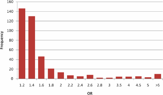
Figure 3: Distribution of validated effect sizes identified in case-control GWAS 56 for a range of common diseases.

When the results of GWAS are published they usually focus on a few highly significant SNPs. But GWAS also contain information about the overall genetic basis for complex traits, for example, the number of genes affecting a trait, the number of polymorphisms at these genes, their allele frequencies and their effects on the trait. This information is of interest in its own right and is also useful in setting prior distributions such as $p(b)$ used in predicting phenotype. Figure 3 presents the distribution of SNP effects for a range of diseases published to date from GWAS. These estimates are from the validation experiment so that they minimize the bias described above for significant SNPs in the discovery experiment. Typically, SNPs increase the risk of disease by 1.1–1.3. The number of independent SNPs of this effect size needed to explain all the observed genetic variance depends on the allele frequencies of the SNPs and the genetic variance of the trait. Assuming the SNPs that have been discovered and reported are typical in effect size and allele frequencies, 100–1000 SNPs would be needed to explain the genetic variance of the diseases in Table 1 25 . In fact, the SNPs discovered are likely to have larger than average effect sizes and so the total number of genes needed to explain the observed genetic variance is probably very large. Similar conclusions can be reached from the published GWAS on human height. The effect sizes are small (0.1–0.3 cm per allele) and so 100s of such SNPs are needed to explain the genetic variance of height 47 .

There have been no published reports of the accuracy of predicting complex traits from GWAS in humans. However, 41 SNPs associated with human height have been reported from 3 large GWAS. Collectively, these explain only $\sim$6% of the variance, giving a correlation between phenotype of predicted genotype of $\sqrt{(0.06)}=0.23$. This is disappointing and typical of other traits, leading to the question “Where are the missing genes?” 48 . Even when we have attempted to use all available SNPs, we do not observe high correlations (Yang, Goddard, Visscher and others, unpublished).

Goddard (2009) 43 and Hayes et al. (2009) 45 developed analytic methods to calculate the accuracy of prediction of genetic value from markers. A small $N_{e}$, a small number of QTL affecting the trait, a high heritability, a large number of markers and a large number of individuals in the reference sample lead to a high correlation between predicted and true genetic value.

Which of the statistical methods gives the most accurate prediction depends on which distribution of $b$ corresponds most closely to the real world. In the analysis of data on milk production traits in cattle, Van Raden et al. (2008) 46 found that other methods gave only a small improvement over BLUP, implying that many SNPs, each with a small effect, give the best prediction. Lee et al. (2008) 41 , using data on mouse coat color and other quantitative traits and a method similar to Bayes B, found that only a small proportion of markers were needed, as might be expected given the small number of known genes affecting coat color. More markers were needed for two other quantitative traits.

$N_{e}$ in dairy cattle has been about 100 for the last 6–40 generations but was 1000–2000 prior to that 49 . On the other hand, $N_{e}$ in humans went through a bottleneck of about 3000, approximately 500 generations ago, and has since expanded enormously 50 . The recent small $N_{e}$ in cattle has generated some long range LD which increases the accuracy of prediction. The equivalent model described above suggests another way to describe this situation: in cattle there are many individuals that have inherited the same chromosome segment from a common ancestor and the markers track this relationship. In most human populations there are few of these close relationships and so the markers cannot so easily track the inheritance of identical chromosome segments. The mouse data came from the heterogeneous mouse line 51 derived from crossing inbred strains and consequently has long range LD, making it possible for markers to predict genetic value by tracing large chromosome segments.

The milk yield data analyzed by VanRaden et al. (2008) 46 was the average milk yield of the daughters of each bull and, consequently, the heritability of these “phenotypes” is high, approximately 0.8. The heritability of human height is also about 0.8, so this does not explain the lower accuracy of predicting height 52 . However, a number of diseases have lower heritability and this partly explains the difficulty in predicting them. VanRaden et al. (2008) 46 reported that increasing the number of individuals and increasing the number of markers both increased the accuracy of predicting genetic value, as would be expected from the theory described here and elsewhere.

4 Future Developments

The theory in Goddard (2009) 53 and Hayes et al. (2009) 43 is supported by the limited data on the accuracy with which genetic value can be predicted from SNPs. However, the proportion of genetic variance explained by SNPs for human height is still lower than expected, begging the question “Where are the missing genes”? Future research must try to answer this question. The explanation that there is substantial epistasis, or that de novo mutants (including de novo copy number variants) or epigenetic effects are important, is unsatisfactory. The heritability of human height ($\sim$0.8) is the narrow sense heritability, that is, it is the proportion of phenotypic variance that is due to the additive effect of genes. Epistasis does not contribute to the narrow sense heritability, de novo mutations are by definition not inherited and few inherited epigenetic changes are known. In any case, an inherited stable epimutation, for example, a mutation that changes the methylation status at a locus and affects the phenotype, would in practice behave just like a mutation that changes a nucleotide, in terms of the resemblance between relatives and the SNP-phenotype correlation in gene mapping experiments.

There appear to be three possible explanations. First, the genetic markers (i.e., SNPs) may not be tracking the QTL. That is, the SNPs may not be in high enough LD with the QTL. Since we have not identified most of the QTL, we cannot answer this question directly. If we assume that the QTL are similar to SNPs in their properties, we can use the LD between SNPs as a guide to the LD between SNPs and QTL. The SNPs on commercial “SNP chips” are considered to represent about 68–92% of the known common genetic variation when compared to variation in samples representing 120 Caucasian chromosomes genotyped in the human HapMap project 54 . However, near complete sequencing of 76 genes on the same subjects 55 has identified more common variants, suggesting that only 57–79% of common variation is represented by the current generation of SNP chips. Thus, the coverage is good but not perfect. However, QTL may have different properties to SNPs. For example, they may be under stronger selection, and therefore be younger polymorphisms with lower minor allele frequency. This would decrease LD with SNP markers. Alternatively, QTL may often be deletions or duplications of DNA which interfere with the ability to assay SNPs near enough to be in LD with the deletion or duplication. Some copy number variants (DNA sequences which vary between individuals in the number of copies they carry on a chromosome, e.g., insertion/deletion variants) can also be typed using the latest generation of SNP chips.

Second, the variance explained by individual QTL may be so small that experiments with 10,000s of individuals are not powerful enough. The finding in dairy cattle, that a prediction method designed for the situation where all SNPs have small effects performs well, gives some support to this explanation. Even if every one of the $3\times 10^{9}$ bases of DNA had a tiny effect on a trait, LD among these QTL would create “super-loci,” each consisting of a chromosome segment inherited as a block and it would only be necessary to estimate the combined effects of the QTL on this segment. As pointed out by Goddard (2009) 43 , the size of these segments depends on the $N_{e}$ of the population and the recombination rate. The genome can be divided into approximately $4N_{e}L$ segments or effective QTL, where $L$ is the length of the genome in recombination units or Morgans. Thus, a population with a large $N_{e}$ can have a large number of effective QTL but a population with small $N_{e}$ cannot.

Both of these first two explanations of the low accuracy with which genetic value can be predicted from SNPs might apply to humans. The third explanation is that there are some phenomena explaining inheritance of which we are totally unaware.

Assuming that the first two explanations are enough, we should be able to explain a larger proportion of the genetic variance by increasing the number of individuals in the reference sample and by increasing the density of markers. In fact, complete sequencing of the genome is likely to replace or complement genotyping of known polymorphism in the foreseeable future. This should allow causal polymorphisms to be used in prediction instead of linked markers. However, it will also increase the number of variable sites whose effects must be estimated by an order of magnitude or more. Despite this increase in data quantity and quality, the methods of predicting genetic value and of estimating the effect of polymorphisms, discussed in this paper, will still be relevant. We expect that as the number of polymorphisms increases and includes the causal variants, methods of prediction that assume many markers have no effect on the trait will perform better than methods that assume all markers have some effect. This is because we expect markers with no direct effect to cease to be useful predictors when the causal polymorphism, to which they are linked, is included in the model. However, whether the data will be sufficiently powerful to distinguish causal variants from markers in LD with them remains to be seen.

References

- (1) Allison, D. B., Fernandez, J. R., Heo, M., Zhu, S. K., Etzel, C., Beasley, T. M. and Amos, C. I. (2002). Bias in estimates of quantitative-trait-locus effect in genome scans: Demonstration of the phenomenon and a method-of-moments procedure for reducing bias. Am. J. Hum. Genet. 70 575–585.
- (2) Almasy, L. and Blangero, J. (1998). Multipoint quantitative-trait linkage analysis in general pedigrees. Am. J. Hum. Genet. 62 1198–1211.
- (3) Aulchenko, Y. S., Struchalin, M. V., Belonogova, N. M., Axenovich, T. I., Weedon, M. N., Hofman, A., Uitterlinden, A. G., Kayser, M., Oostra, B. A., van Duijn, C. M., Janssens, A. C. and Borodin, P. M. (2009). Predicting human height by Victorian and genomic methods. Eur. J. Hum. Genet. 17 1070–1075.
- (4) Beavis, W. D. (1988). QTL analyses: Power, precision and accuracy. Molecular Dissection of Complex Traits (A. H. Paterson, ed.) 145–162. CRC Press, New York.
- (5) Beavis, W. D. (1994). The power and deceit of QTL experiments: Lessons from comparative QTL studies. In Proceedings of the Forty-ninth Annual Corn and Sorghum Industry Research Conference 250–266. American Seed Trade Association, Washington, DC.
- (6) Bhangale, T. R., Rieder, M. J. and Nickerson, D. A. (2008). Estimating coverage and power for genetic association studies using near-complete variation data. Nature Genetics 40 841–843.
- (7) Bogdan, M. and Doerge, R. W. (2005). Biased estimators of quantitative trait locus heritability and location in interval mapping. Heredity 95 476–484.
- (8) Casella, G. and Berger, R. L. (1990). Statistical Inference. Duxbury Press, Belmont. \MR1051420
- (9) de Roos, A. P. W., Hayes, B. J., Spelman, R. J. and Goddard, M. E. (2008). Linkage disequilibrium and persistence of phase in Holstein–Friesian, Jersey and Angus cattle. Genetics 179 1503–1512.
- (10) Fernando, R. L. and Gianola D. (1986). Optimal properties of the conditional mean as a selection criterion. Theor. Appl. Genet. 72 822–825.
- (11) Foster, S. D., Verbyla, A. P. and Pitchford, W. S. (2007). Incorporating LASSO effects into a mixed model for quantitative trait loci detection. Journal of Agricultural Biological and Environmental Statistics 12 300–314. \MR2370788
- (12) Foster, S. D., Verbyla, A. P. and Pitchford, W. S. (2008). A random model approach for the LASSO. Comput. Statist. 23 217–233. \MR2399114
- (13) Frazer, K. A., Ballinger, D. G., Cox, D. R., Hinds, D. A., Stuve, L. L., Gibbs, R. A., Belmont, J. W., Boudreau, A., Hardenbol, P., Leal, S. M., Pasternak, S., Wheeler, D. A., Willis, T. D., Yu, F. L., Yang, H. M., Zeng, C. Q., Gao, Y., Hu, H. R., Hu, W. T., Li, C. H., Lin, W., Liu, S. Q., Pan, H., Tang, X. L., Wang, J., Wang, W., Yu, J., Zhang, B., Zhang, Q. R., Zhao, H. B., Zhao, H., Zhou, J., Gabriel, S. B., Barry, R., Blumenstiel, B., Camargo, A., Defelice, M., Faggart, M., Goyette, M., Gupta, S., Moore, J., Nguyen, H., Onofrio, R. C., Parkin, M., Roy, J., Stahl, E., Winchester, E., Ziaugra, L., Altshuler, D., Shen, Y., Yao, Z. J., Huang, W., Chu, X., He, Y. G., Jin, L., Liu, Y. F., Shen, Y. Y., Sun, W. W., Wang, H. F., Wang, Y., Xiong, X. Y., Xu, L., Waye, M. M. Y., Tsui, S. K. W., Wong, J. T. F., Galver, L. M., Fan, J. B., Gunderson, K., Murray, S. S., Oliphant, A. R., Chee, M. S., Montpetit, A., Chagnon, F., Ferretti, V., Leboeuf, M., Olivier, J. F., Phillips, M. S., Roumy, S., Sallee, C., Verner, A., Hudson, T. J., Kwok, P. Y., Cai, D. M., Koboldt, D. C., Miller, R. D., Pawlikowska, L., Taillon-Miller, P., Xiao, M., Tsui, L. C., Mak, W., Song, Y. Q., Tam, P. K. H., Nakamura, Y., Kawaguchi, T., Kitamoto, T., Morizono, T., Nagashima, A., Ohnishi, Y., Sekine, A., Tanaka, T., Tsunoda, T., Deloukas, P., Bird, C. P., Delgado, M., Dermitzakis, E. T., Gwilliam, R., Hunt, S., Morrison, J., Powell, D., Stranger, B. E., Whittaker, P., Bentley, D. R., Daly, M. J., de Bakker, P. I. W., Barrett, J., Chretien, Y. R., Maller, J., McCarroll, S., Patterson, N., Pe’er, I., Price, A., Purcell, S., Richter, D. J., Sabeti, P., Saxena, R., Schaffner, S. F., Sham, P. C., Varilly, P., Stein, L. D., Krishnan, L., Smith, A. V., Tello-Ruiz, M. K., Thorisson, G. A., Chakravarti, A., Chen, P. E., Cutler, D. J., Kashuk, C. S., Lin, S., Abecasis, G. R., Guan, W. H., Li, Y., Munro, H. M., Qin, Z. H. S., Thomas, D. J., McVean, G., Auton, A., Bottolo, L., Cardin, N., Eyheramendy, S., Freeman, C., Marchini, J., Myers, S., Spencer, C., Stephens, M., Donnelly, P., Cardon, L. R., Clarke, G., Evans, D. M., Morris, A. P., Weir, B. S., Johnson, T. A., Mullikin, J. C., Sherry, S. T., Feolo, M., Skol, A. and Int HapMap, C. (2007). A second generation human haplotype map of over 3.1 million SNPs. Nature 449 851–861.
- (14) Ghosh, A., Zou, F. and Wright, F. A. (2008). Estimating odds ratios in genome scans: An approximate conditional likelihood approach. Am. J. Hum. Genet. 82 1064–1074.
- (15) Gianola, D., Fernando, R. L. and Stella, A. (2006). Genomic-assisted prediction of genetic value with semiparametric procedures. Genetics 173 1761–1776.
- (16) Goddard, M. E. (1991). Mapping genes for quantitative traits using linkage disequilibrium. Genetics Selection and Evolution 23 S131–S134.
- (17) Goddard, M. E. (2009). Genomic selection: Prediction of accuracy and maximisation of long term response. Genetica 136 245–257.
- (18) Goring, H. H. H., Terwilliger, J. D. and Blangero, J. (2001). Large upward bias in estimation of locus-specific effects from genomewide scans. Am. J. Hum. Genet. 69 1357–1369.
- (19) Green, P. J. (1995). Reversible jump Markov chain Monte Carlo computation and Bayesian model determination. Biometrika 82 711–732. \MR1380810
- (20) Hayes, B. J., Bowman, P. J., Chamberlain, A. J. and Goddard, M. E. (2009). Invited review: Genomic selection in dairy cattle: Progress and challenges. Journal of Dairy Science 92 433–443.
- (21) Hayes, B. J., Gjuvsland, A. and Omholt, S. (2006). Power of QTL mapping experiments in commercial Atlantic salmon populations, exploiting linkage and linkage disequilibrium and effect of limited recombination in males. Heredity 97 19–26.
- (22) Hayes, B. J., Visscher, P. M. and Goddard, M. E. (2009). Increased accuracy of artificial selection by using the realised relationship matrix. Genetics Research 91 47–60.
- (23) Henderson, C. R. (1950). Estimation of genetic parameters. Ann. Math. Stat. 21 309–310.
- (24) Henderson, C. R. (1973). Sire evaluation and genetic trends. In: Proceedings of the Animal Breeding and Genetics Symposium in Honor of Dr. J. L. Lush; 1973 10–41. American Society of Animal Science, Campaign, IL.
- (25) Henderson, C. R. (1975). Best linear unbiased estimation and prediction under a selection model. Biometrics 31 423–449.
- (26) Hill, W. G., Goddard, M. E. and Visscher, P. M. (2008). Data and theory point to mainly additive genetic variance for complex traits. Plos Genetics 4 1–10.
- (27) Hindorff, L. A., Junkins, H. A., Mehta, J. P. and Manolio, T. A. (2009). A catalog of published genome-wide association studies. Available at www.genome.gov/26525384.
- (28) Hoggart, C. J., Whittaker, J. C., De Iorio, M. and Balding, D. J. (2008). Simultaneous analysis of all SNPs in genome-wide and re-sequencing association studies. PLoS Genet. 4 e1000130.
- (29) Kruuk, L. E. B. (2004). Estimating genetic parameters in natural populations using the “animal model.” Philosophical Transactions of the Royal Society of London Series B—Biological Sciences 359 873–890.
- (30) Lande, R. and Thompson, R. (1990). Efficiency of marker-assisted selection in the improvement of quantitative traits. Genetics 124 743–756.
- (31) Lee, S. H., van der Werf, J. H. J., Hayes, B. J., Goddard, M. E. and Visscher, P. M. (2008). Predicting unobserved phenotypes for complex traits from whole-genome SNP data. Plos Genetics 4 1–11.
- (32) Lewinger, J. P., Conti, D. V., Baurley, J. W., Triche, T. J. and Thomas, D. C. (2007). Hierarchical Bayes prioritization of marker associations from a genome-wide association scan for further investigation. Genet. Epidemiol. 31 871–882.
- (33) Lynch, M. and Walsh, B. (1998). Genetics and Analysis of Quantitative Traits. Sinauer, Sunderland, MA.
- (34) Maher, B. (2008). Personal genomes: The case of the missing heritability. Nature 456 18–21.
- (35) McCarthy, M. I., Abecasis, G. R., Cardon, L. R., Goldstein, D. B., Little, J., Ioannidis, J. P. A. and Hirschhorn, J. N. (2008). Genome-wide association studies for complex traits: Consensus, uncertainty and challenges. Nature Reviews Genetics 9 356–369.
- (36) Meuwissen, T. H. E., Hayes, B. J. and Goddard, M. E. (2001). Prediction of total genetic value using genome-wide dense marker maps. Genetics 157 1819–1829.
- (37) Robinson, G. K. (1991). That BLUP is a good thing: The estimation of random effects. Statist. Sci. 6 15–32. \MR1108815
- (38) Siegmund, D. (2002). Upward bias in estimation of genetic effects. Am. J. Hum. Genet. 71 1183–1188.
- (39) Skol, A. D., Scott, L. J., Abecasis, G. R. and Boehnke, M. (2006). Joint analysis is more efficient than replication-based analysis for two-stage genome-wide association studies. Nature Genetics 38 209–213.
- (40) Sorenson, P. and Gianola, D. (2002). Likelihood, Bayesian, and MCMC Methods in Quantitative Genetics. Springer, New York. \MR1919970
- (41) Sun, L. and Bull, S. B. (2005). Reduction of selection bias in genomewide studies by resampling. Genet. Epidemiol. 28 352–367.
- (42) Tenesa, A., Navarro, P., Hayes, B. J., Duffy, D. L., Clarke, G. M., Goddard, M. E. and Visscher, P. M. (2007). Recent human effective population size estimated from linkage disequilibrium. Genome Research 17 520–526.
- (43) Thompson, R. (1979). Sire evaluation. Biometrics 35 339–353.
- (44) Tibshirani, R. (1996). Regression shrinkage and selection via the Lasso. J. R. Stat. Soc. Ser. B Stat. Methodol. 58 267–288. \MR1379242
- (45) Utz, H. F., Melchinger, A. E. and Schon, C. C. (2000). Bias and sampling error of the estimated proportion of genotypic variance explained by quantitative trait loci determined from experimental data in maize using cross validation and validation with independent samples. Genetics 154 1839–1849.
- (46) Valdar, W., Solberg, L. C., Gauguier, D., Cookson, W. O., Rawlins, J. N. P., Mott, R. and Flint, J. (2006). Genetic and environmental effects on complex traits in mice. Genetics 174 959–984.
- (47) VanRaden, P. M. (2008). Efficient methods to compute genomic predictions. Journal of Dairy Science 91 4414–4423.
- (48) Visscher, P. M. (2008). Sizing up human height variation. Nature Genetics 40 489–490.
- (49) Visscher, P. M., Medland, S. E., Ferreira, M. A. R., Morley, K. I., Zhu, G., Cornes, B. K., Montgomery, G. W. and Martin, N. G. (2006). Assumption-free estimation of heritability from genome-wide identity-by-descent sharing between full siblings. Plos Genetics 2 316–325.
- (50) Visscher, P. M., Thompson, R., Haley, C. S. (1996). Confidence intervals in QTL mapping by bootstrapping. Genetics 143 1013–1020.
- (51) Weller, J. I., Shlezinger, M. and Ron, M. (2005). Correcting for bias in estimation of quantitative trait loci effects. Genetics Selection Evolution 37 501–522.
- (52) Wray, N. R., Goddard, M. E. and Visscher, P. M. (2007). Prediction of individual genetic risk to disease from genome-wide association studies. Genome Res. 17 1520–1528.
- (53) Xu, S. Z. (2003). Theoretical basis of the Beavis effect. Genetics 165 2259–2268.
- (54) Zhong, H. and Prentice, R. L. (2008). Bias-reduced estimators and confidence intervals for odds ratios in genome-wide association studies. Biostatistics 9 621–634.
- (55) Zollner, S. and Pritchard, J. K. (2007). Overcoming the winner’s curse: Estimating penetrance parameters from case-control data. Am. J. Hum. Genet. 80 605–615.
- (56) WTCCC (2007). Genome-wide association study of 14,000 cases of seven common diseases and 3,000 shared controls. Nature 447 661–678.