First results for $B_{K}$ on the ultrafine ($a=0.045$ fm) ensemble

Abstract:

We present preliminary results for $B_{K}$ from the MILC ultrafine lattices, based on a partial ensemble of 305 configurations. We use HYP-smeared improved staggered valence quarks. The analysis is done using fitting forms based on both SU(2) and SU(3) staggered chiral perturbation thery. For the SU(2) analysis, we find that the result using the NLO fit function is consistent with that from a partial NNLO fit. For the SU(3) analysis, where we have to use partially constrained fits due to the number of fit parameters, we find that our two preferred fits (“N-BB1” and “N-BB2”) are also consistent, both with each other and with the results of the SU(2) fits. These results are used in companion proceedings to improve the control over the continuum extrapolation.

1 Introduction

This paper is the last of four proceedings [1, 2, 3] describing our calculation of $B_{K}$ using improved staggered fermions. Here, we present our first results using the MILC “ultrafine” ensemble, with $a=0.045$ fm. This is the finest of four lattice spacings that we have used, the others being the “coarse” ($a=0.12$ fm), “fine” ($a=0.09$ fm) and “superfine” ($a=0.06$ fm) spacings. Our previous result for $B_{K}$ was based on these three spacings [4]. Having a fourth point closer to the continuum limit both checks our previous continuum extrapolation and reduces the error in that extrapolation.

The parameters for the numerical study are collected in Table 1. As can be seen, we have so far obtained results on only 305 configurations, less than half of the total available. Hence, the results are preliminary.

parameter	value
sea quarks	asqtad staggered fermions
valence quarks	HYP-smeared staggered fermions
geometry	$64^{3}\times 192$
number of confs.	305
$am_{l}/am_{s}$	$0.0028/0.014$
$1/a$	4517 MeV
$\alpha_{s}$	0.2096 for $\mu=1/a$
$am_{x}$, $am_{y}$	$0.0014\times n$ ($n=1,2,3,\ldots,10$)

Table 1: Parameters for the numerical study on the ultrafine (U1) ensemble. $m_{l}$ is the light sea quark mass, $m_{s}$ the strange sea quark mass, $m_{x}$ the light valence quark mass, and $m_{y}$ the strange valence quark mass.

2 Extracting $B_{K}$

We calculate $B_{K}$ using the methods described in Ref. [4]. We place the U(1) noise wall-sources at $t=0$ and $t=80$. These sources couple only to the Goldstone-taste pion ($\xi_{5}$). In Fig. 1, we show an example of our results for the ratio of matrix elements which equals $B_{K}$ when the operator (placed at time $T$) is far from both sources. We choose the fitting range such that the excited states with the same quantum numbers as the Goldstone pion mode do not make significant contributions, as determined from wall-source to current correlators. In this case, we choose the fitting range to be $25\leq t\leq 54$, and fit to a constant, as in the example shown in Fig. 1.

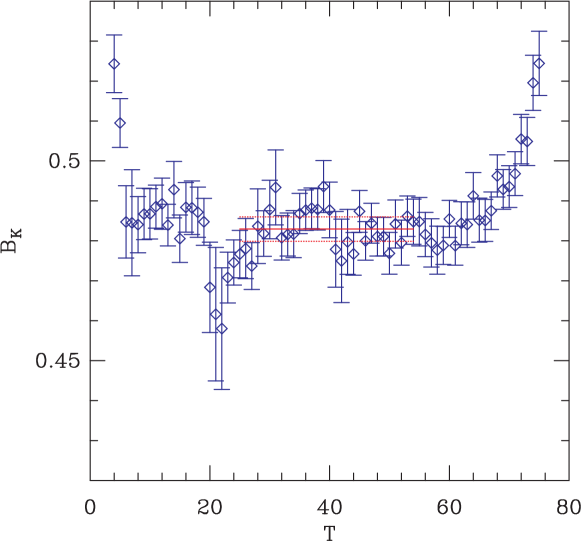
Figure 1: $B_{K}$ versus $T$ on the ultrafine ensemble, obtained using one-loop matching with renormalization scale $\mu=1/a$. Valence masses are $am_{x}=am_{y}=0.007$, corresponding to a kaon with approximately the physical mass.

3 SU(2) SChPT analysis

Our most reliable method of extrapolating $B_{K}$ to the physical quark masses is based on SU(2) staggered chiral perturbation theory (SChPT). The resulting fit forms and a detailed description of our fitting method are given in Ref. [4]. In brief, the fits are done in two steps.

1. In the “X-fit” we extrapolate $m_{x}\to m_{d}^{\rm phys}$, with $m_{y}$ fixed, while at the same time using the SChPT fit form to remove taste-breaking lattice artifacts, and to set $m_{\ell}\to m_{\ell}^{\rm phys}$ in the chiral logarithms. The fit function takes the form [4]

   $$f_{\text{th}} = d_{0}F_{0}+d_{1}\frac{X_{P}}{\Lambda_{\chi}^{2}}+d_{2}\frac{X_{P}^{2}}{\Lambda_{\chi}^{4}}\,,$$ (1)

   where $X_{P}$ is the mass of the pion composed of valence quarks of mass $m_{x}$, and $F_{0}=1+\text{chiral logs}$. The chiral logarithms have a known form in terms of measurable pion masses. The coefficient $d_{2}$ multiplies an analytic next-to-next-to-leading order (NNLO) term. The coefficients $d_{0}-d_{2}$ are expected to have $O(1)$ magnitudes.

2. In the “Y-fit”, we extrapolate the results of the X-fits to $m_{y}=m_{s}^{\rm phys}$, using an analytic fit function. A linear Y-fit appears sufficient, and we use this for our central value.

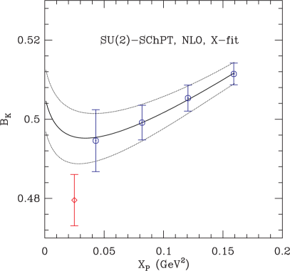
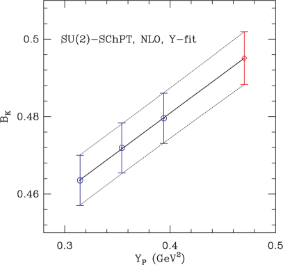
Figure 2: $B_{K}$ versus $X_{P}$ (mass of the pion composed of valence quarks of mass $m_{x}$) and corresponding 4X-NLO fit (left panel) and $B_{K}$ versus $Y_{P}$ (mass of pion composed of quarks of mass $m_{y}$) along with the 3Y linear fit (right panel). $B_{K}(\mu=1/a)$ is obtained using one-loop matching. In the left panel, $am_{y}=0.014$, and the red point is the result of setting $m_{x}=m_{d}^{\rm phys}$, $m_{\ell}=m_{\ell}^{\rm phys}$ and removing taste breaking.

In Fig. 2, we show an example of both X- and Y-fits. We use our lightest four values of $m_{x}$ in the X-fits and our heaviest three values of $m_{y}$ in the Y-fits. Furthermore, the fit function for the X-fit is of NLO. Thus the fit is labeled 4X3Y-NLO. The corresponding plots for NNLO X-fits, in which we add a single analytic NNLO term [4], are shown in Fig. 3. Illustrative parameters from these fits are collected in Table 2. Note that, since we use an uncorrelated $\chi^{2}/{\rm d.o.f}$, we expect values much smaller than unity if the fit is good.

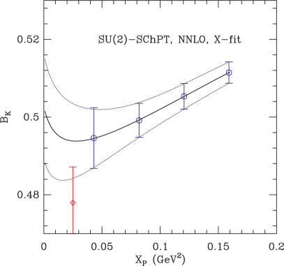
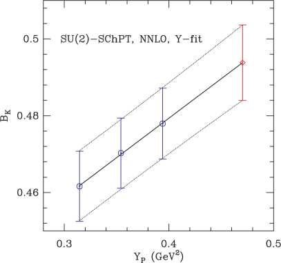
Figure 3: As for Fig. 2, but using NNLO X-fits.

fit	$d_{0}$	$d_{1}$	$d_{2}$	$\chi^{2}/\text{d.o.f}$	$B_{K}(\mu=1/a)$
4X3Y-NLO	0.4702(73)	0.155(40)	—	0.017(66)	0.4951(68)
4X3Y-NNLO	0.4973(126)	0.22(17)	$-$0.26(57)	0.0012(99)	0.4938(98)

Table 2: X-fit parameters for the 4X-NLO and 4X-NNLO fits shown in the left panels of Figs. 2 and 3, and results for $B_{K}$ after the Y-fits shown in the right panels.

We can see from the figures and the Table that the difference between values for $B_{K}$ resulting from these fits is very small. We also see that, although $d_{0}$ is well determined, $d_{1}$ and $d_{2}$ are not. The poor determination of $d_{1}$ and $d_{2}$ has, however, little impact on our extrapolated value.

An important feature of the fitting function is the presence of chiral logarithms, which lead to the curvature for small $X_{P}$. While our data is consistent with this curvature, it is very small in the region of our points, and our data itself provides no direct evidence for the presence of chiral logarithms.

Finally, we note that the convergence of SU(2) ChPT is satisfactory for all points included in the fits. This can be seen, for example, by the closeness of $d_{0}$ to the values of $B_{K}$ to which we fit.

4 SU(3) Analysis

The SU(3) fits have the advantage of using all our data points (55 mass pairs), but two disadvantages. These are that the convergence of SU(3) ChPT is questionable for many of our points, and that the NLO SU(3) SChPT fit forms are much more involved. We sketch the situation here, and refer to Ref. [4] for details.

Compared to the SU(2) fits, we have to make two simplifications in order to obtain stable fits. First, we need to lump together classes of fit functions which have similar functional forms, using only one function as representative. Second, we need to use constrained (Bayesian) fitting—parameters associated with taste-breaking are constrained to lie in the range of values expected from SChPT power counting. With these simplifications we were able to obtain good fits on the coarse, fine and superfine ensembles [4]. We found, however, that different assumptions about the constraints led to significant variation in the final answer for $B_{K}$, and this gave rise to a large systematic error. The particular value for this error quoted in [4], which was 5.3%, came from the analysis on the coarse ensemble C3. Thus it is interesting to see whether the variation between fits is reduced on the ultrafine lattices. We would expect significant reduction because the offending terms in the fit functions are proportional to either $a^{2}$ or $\alpha_{s}(1/a)^{2}$.

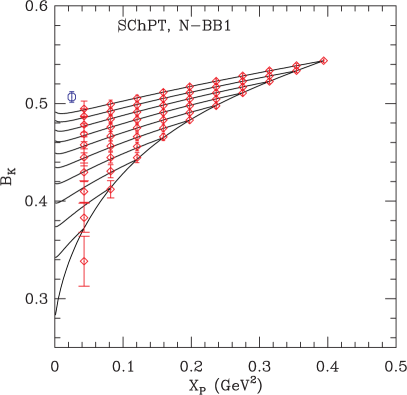
Figure 4: One-loop matched $B_{K}$ versus $X_{P}$ on the U1 lattice for the D-B1 fit (left) and for the N-BB1 fit (right). The fits are described in the text and, in more detail, in Ref. [4]. The blue octagon in the right-hand plot shows the result after extrapolation to physical quark masses and after removing lattice artifacts.

In Fig. 4, we show the results of two fits. That shown on the left is a “D-B1” fit, in which we use only degenerate kaons, and constrain the representative lattice artifact term based on the assumption that it is proportional to $a^{2}$. The fit in the right panel is a “D-BB1” fit to the entire data set, with two Bayesian constraints. The first constraint is that the results (including errors) of the D-B1 fit are used to constrain the parameters that contribute for degenerate kaons. The second is that additional representative lattice artifact terms are constrained based on the assumption that they are proportional to $a^{2}$.

In Fig. 5, we show the $B_{K}$ results of two different fits: D-B2 on the left and N-BB2 on the right. These differ from D-B1 and N-BB1 in that lattice artifact terms are presumed to be proportional to $\alpha_{s}^{2}$ rather than $a^{2}$. The results for $B_{K}(1/a)$, after removal of taste-breaking from the chiral logarithms, and after extrapolation to physical quark masses, are given in Table 3.

fit type	$\chi^{2}/\text{d.o.f}$	$B_{K}(\mu=1/a)$
N-BB1	0.075(81)	0.5067(55)
N-BB2	0.052(38)	0.5127(76)

Table 3: Results for $B_{K}$ and fit quality from N-BB1 and N-BB2 fits on the U1 ensemble.

We see that the difference between N-BB1 and N-BB2 fits has been reduced to 1.2%, compared to the 5.3% found on the C3 ensemble. We interpret this improvement as being due to the reduction in the size of taste-breaking effects. As Table 4 shows, if these effects are dominantly discretization errors, the expected reduction in their size is $\sim 7.5$, while if they are dominantly truncation errors the reduction is $\sim 2.5$. Thus, as far as the need for Bayesian constraints goes, the move to smaller lattice spacings improves the stability of the SU(3) fitting. The only caveat to this statement is that a similar reduction is not observed on the S1 ensemble [4].

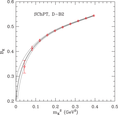
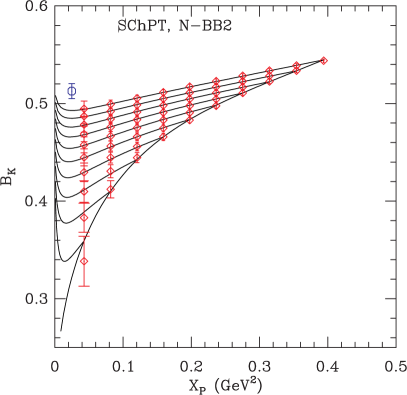
Figure 5: As for Fig. 4, except using D-B2 (left) and N-BB2 (right) fits.

parameter	C3	U1
$a^{2}$ (fm2)	0.0141	0.0019
$\alpha_{s}^{2}(\mu=1/a)$	0.1080	0.0439

Table 4: $a^{2}$ and $\alpha_{s}^{2}$ for the C3 and U1 lattices.

5 Conclusion

As one can see from Tables 2 and 3, the results from the SU(2) fits lie below those from the SU(3) fits. This difference is not, however, statistically significant. For example, using our preferred 4X3Y-NNLO and N-BB1 fits, the difference is only $1.2\sigma$. Although the error on the SU(3) N-BB1 fit is nominally smaller than that on the SU(2) 4X3Y-NNLO fit, we think that the latter fit is more reliable, as discussed above and in Ref. [4].

Although our results use somewhat less than half of the 883 ultrafine configurations that we intend to analyze, we can already see that fitting simplifies as we approach the continuum limit, and systematic errors are correspondingly reduced. This is particularly true of the SU(3) fitting. However, one should keep in mind that one does not expect the chiral convergence of SU(3) fitting to improve on finer lattices.

The data presented here is incorporated into continuum extrapolations in two of the companion proceedings [1, 2].

6 Acknowledgments

C. Jung is supported by the US DOE under contract DE-AC02-98CH10886. The research of W. Lee is supported by the Creative Research Initiatives Program (3348-20090015) of the NRF grant funded by the Korean government (MEST). The work of S. Sharpe is supported in part by the US DOE grant no. DE-FG02-96ER40956. Computations were carried out in part on QCDOC computing facilities of the USQCD Collaboration at Brookhaven National Lab. The USQCD Collaboration are funded by the Office of Science of the U.S. Department of Energy.

References

- [1] Boram Yoon, et al. PoS (LATTICE 2010) 319; [arXiv:1010.4778].
- [2] Jangho Kim, et al. PoS (LATTICE 2010) 310; [arXiv:1010.4779].
- [3] Yong-Chull Jang, et al. PoS (LATTICE 2010) 229; [arXiv:1010.4780].
- [4] Taegil Bae, et al., [arXiv:1008.5179].