The Dynamic Scaling Study of Vapor Deposition Polymerization: A Monte Carlo Approach

Abstract

The morphological scaling properties of linear polymer films grown by vapor deposition polymerization (VDP) are studied by 1+1D Monte Carlo simulations. The model implements the basic processes of random angle ballistic deposition ($F$), free-monomer diffusion ($D$) and monomer adsorption along with the dynamical processes of polymer chain initiation, extension, and merger. The ratio $G=D/F$ is found to have a strong influence on the polymer film morphology. Spatial and temporal behavior of kinetic roughening has been extensively studied using finite-length scaling and height-height correlations $H(r,t)$. The scaling analysis has been performed within the no-overhang approximation and the scaling behaviors at local and global length scales were found to be very different. The global and local scaling exponents for morphological evolution have been evaluated for varying free-monomer diffusion by growing the films at $G$ = $10$, $10^{2}$, $10^{3}$, and $10^{4}$ and fixing the deposition flux $F$. With an increase in $G$ from $10$ to $10^{4}$, the average growth exponent $\beta\approx 0.50$ was found to be invariant, whereas the global roughness exponent $\alpha_{g}$ decreased from $0.87(1)$ to $0.73(1)$ along with a corresponding decrease in the global dynamic exponent $z_{g}$ from $1.71(1)$ to $1.38(2)$. The global scaling exponents were observed to follow the dynamic scaling hypothesis, $z_{g}=\alpha_{g}/\beta$. With a similar increase in $G$ however, the average local roughness exponent ${\alpha_{l}}$ remained close to $0.46$ and the anomalous growth exponent ${\beta}_{\ast}$ decreased from 0.23(4) to 0.18(8). The interfaces display anomalous scaling and multiscaling in the relevant height-height correlations. The variation of $H(r,t)$ with deposition time $t$ indicates non-stationary growth. A comparison has been made between the simulational findings and the experiments wherever applicable.

I INTRODUCTION

Our motivation for gaining theoretical understanding of polymer thin film growth stems from their technological applications in microelectronic interconnects Lu and Moore (1997); Wong (1993), organic electronics Wong (1993), and biotechnology. Various experimental methods like vapor deposition polymerization (VDP) Lu and Moore (1997); Gorham (1966); Lahann et al. (2003); Szulczewski et al. (2000), ionization assisted polymer deposition Usui (1998), sputtering growth Biederman et al. (2003), pulsed laser deposition Chrisey and Hubler (1994); Piqu et al. (2003), and organic molecular beam deposition Schreiber (2004) have been developed to produce a variety of polymer thin films. Polymer film growth is complex compared to the conventional inorganic thin film growth process due to polymer’s complicated structure and interactions that include internal degrees of freedom, limited bonding sites, chain-chain interactions, etc. Many experimental efforts have focussed on the formation of polymer thin films using VDP Collins et al. (1994); Biscarini et al. (1997); Fortin and Lu (2002). In a typical VDP experiment, a wafer (2-D substrate) is exposed to one or more volatile gas phase precursors that produce free-monomers. The free-monomers impinge on the substrate at random locations and react on the substrate surface to produce the desired deposit. Polymer thin films grown by VDP are made up of long polymer chains formed through the polymerization reaction occurring during the growth process. The polymerization process involves the interaction of two free-monomer molecules in a chemical reaction to initiate a dimer (polymer chain of length = 2). The free-monomers moving towards the substrate are consumed by either of the two processes: first being chain initiation in which new polymer molecules are generated; and secondly, chain propagation in which the existing polymer molecules are extended to higher molecular weight. Besides these two mechanisms, the free-monomer adsorption, diffusion, and polymer merger can be considered as other mechanisms that determine the overall film morphology. The chemical nature of the linear polymer chain restricts the number of bonding sites. A free-monomer can only bond to either of the two active ends of a polymer, or to another free-monomer. This bonding constraint leads to the formation of an entangled or an overhang configuration, which blocks the region it covers from the access of other incoming free-monomers. In conventional physical vapor deposition (PVD) processes Mattox (1998), atoms can nucleate at the nearest neighbors of the nucleated sites and atomistic processes such as surface diffusion, edge diffusion, step barrier effect, etc. effect the growth, resulting in the films being compact and denseBarabasi and Stanley (1995); Meakin (1998); Pal and Landau (1994); Shim et al. (1998). Recent investigations by Zhao et al. Zhao et al. (1999a) have shown that the submonolayer growth behavior of VDP is very different from that of PVD due to long chain confinement and limited bonding sites, indicating that the detailed molecular configuration can drastically change the growth behavior Bowie and Zhao (2004). In experiments, the growth behavior of polymer thin films have been investigated through their morphological evolution study. The VDP processes for producing Parylene-N (PA-N) films typically are far from equilibrium. The precursor material di-p-xylylene (dimer) is sublimed at $150^{\circ}$C and then pyrolized into free-monomers at $650^{\circ}$C. The free-monomers impinge at random angles onto the Si-wafer at room temperature and eventually condense and polymerize to form the polymer film. By varying the growth rates in the PA-N growth experiments, Zhao et al.  Zhao et al. (2000) reported an average roughness exponent $\alpha=0.72\pm 0.05$ and an average growth exponent $\beta=0.25\pm 0.03$. However, by considering the tip effect of the atomic force microscope Aue and De Hosson (1997), the range of $\alpha$ was estimated to be between $0.5$ to $0.7$ and the authors found the absence of dynamic scaling hypothesis in the PA-N film growth. In the recent experiments done by Lee et al. Lee et al. (2008), the authors observed unusual changes in the roughening behavior during the poly(chloro-p-xylylene) growth. In the early rapid growth regime, they observed $\beta=0.65$ (larger than the random deposition $\beta=0.5$) and upon complete coverage of the substrate (around $d=10nm$), they found $\beta=0.0$ and the interface width did not evolve with the film thickness. Finally, during the continuous growth regime, the surface roughness again was found to increase steadily with a new power law of $\beta=0.18$ Lee et al. (2008), which is close to the results of Zhao et al. Zhao et al. (2000). Of the known theoretical results for dynamic roughening, the MBE nonlinear surface diffusion dynamics proposed by Lai and Das Sarma Lai and Das Sarma (1991) predicted similar exponents as obtained in the experimental study of Zhao. et al. Zhao et al. (2000). However, their nonlinear surface diffusion theory could not explain the findings of varying local slope in the experiments. Zhao et al. proposed a stochastic growth model based on bulk diffusion Zhao et al. (1999a), which correctly predicted the kinetic roughening phenomena observed in their experiment Zhao et al. (2000) but lacks the details on how polymers evolve. Insufficient theoretical studies coupled with inconsistencies in the experiments motivate us to model the polymer film growth and seek a better understanding of the growth processes that determine the roughening mechanism. In this paper, we study the 1+1D lattice model for the polymer films grown by VDP and examine the effects of random angle deposition, free-monomer diffusion, free-monomer adsorption in determining the evolution of the film’s morphology.

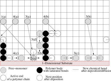
Figure 1: Schematic of the 1+1D growth model. 1(a): Free-monomer deposition at random angles; 2(a): Adsorbed free-monomer diffuses along along the substrate; 2(b): Adsorbed free-monomer diffuses on a polymer chain; 3(a,b): Polymer chain initiation resulting from random angle deposition; 3(c,d): Polymer chain initiation resulting from free-monomer diffusion on substrate and polymer chain respectively; 4(a,b): Free-monomer deposits onto the active end of a polymer chain resulting in chain propagation; 4(c) Chain propagation due to free-monomer diffusion.

II MODEL AND METHOD

In our simulation, the free-monomers were deposited at random angles on a 1-D substrate of lattice size $L$ at a deposition rate $F$ (in units of monomers per site per unit time). The KISS random number generator Marsaglia (2003) was employed and one deposition time unit corresponded to the deposition of $L$ free-monomers. The incident free-monomers were released from a height three lattice units above the highest point on the surface with an initial abscissa randomly chosen from $1\leq x\leq L$. The depositing free-monomers have a uniform “launch angle” distribution which corresponds to a nonuniform flux distribution $J(\theta)\sim 1/cos(\theta)$ of particles above the surface, where $\theta$ is defined as the angle between the direction of impinging monomer and the substrate normal Yu and Amar (2002); Drotar et al. (2000). Our VDP growth model is similar to the square-lattice disk model studied by Ref. Yu and Amar (2002) along with additional constraints of free-monomer diffusion, limited bonding, polymer-initiation, propagation and merger. The particles followed a ballistic trajectory until contacting the surface. The impinging free-monomer was then moved to the lattice position nearest to the point of contact. The deposited free-monomers were allowed to diffuse via nearest-neighbor hops with a diffusion rate $D$ (nearest neighbor hops per monomer per unit time). A free-monomer that is deposited on top of an existing polymer chain gets adsorbed on the chain and is also allowed to diffuse. The excluded volume constraint was implemented by rejecting the diffusion or deposition moves to an already occupied site. As the monomer coverage increases on the substrate, the polymer film grows along a direction perpendicular to the substrate. This “two dimensional” growth is often referred to as the 1+1D growth in literature.

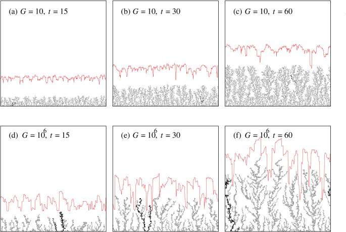
Figure 2: Snapshots of the polymer films grown on a $L$ = $512$ substrate. Figs. (a, b, c) were obtained for $G$ = 10 at deposition times $t$ = 15, 30, and 60 units respectively; whereas Figs. (d, e, f) were obtained for $G$ = $10^{6}$ and deposition times $t$ = 15, 30, and 60 units, respectively. One deposition time unit corresponds to a deposition of $L$ free-monomers. For a clear view, the growth front (shown in red) is displaced vertically by 100 pixels and the longest polymer chain is highlighted in black.

Figure 1 shows the schematic of various processes that occur during the non-equilibrium film growth on a 1-D substrate of length $L$ with periodic boundary conditions. Processes 1(a), 3(a), 3(b), 4(a), and 4(b) show the gas phase free-monomers depositing onto the substrate at random locations with uniform launch angle distribution. These free-monomers get adsorbed either on the substrate (shown by process 2(a)) or on the polymer chains (process 2(b)). Adsorbed free-monomers are allowed to diffuse along the adsorbent to any of the nearest-neighboring unoccupied sites with equal probability, the rate of diffusion $D$ is assumed to be the same on both the substrate and the polymer chain. We define the chain length $s$ of a polymer as the number of monomers forming a polymer chain. When an impinging free-monomer encounters another free-monomer on the substrate as its nearest neighbor (process 3(a)), both are frozen and undergo a chemical reaction to form a dimer (polymer chain of length $s=2$); polymers with chain length $s=3$ can also be formed after deposition (process 3(b)). Free-monomer diffusion along the substrate (process 3(c)) and along the polymer chain (process 3(d)) can also result in the polymer chain initiation Beach (1977). When an impinging free-monomer encounters the active end of a polymer chain, it attaches itself to the chain and increases the chain length by one unit (4(a), 4(b)). A diffusing free-monomer can meet an active end of a polymer chain in its neighborhood and get bonded to that polymer chain (process 4(c)). In linear polymer systems, the free-monomers are allowed to form a maximum of two chemical bonds and at any given time only the two ends of the polymer chain are chemically active, resulting in the chain propagation at these two end locations. The chain portion (of the polymer) excluding the two chemically active ends, is not allowed to form chemical bonds with neighboring free-monomers. Free-monomers can however be physically adsorbed on the chain and can diffuse along the chain (process 2(b)). Another interesting process that occurs during the film growth is the polymer-merger. Two different polymers can merge when their respective active-ends meet as nearest neighbors. During the polymer-merger, the nearest neighboring ends of merging polymers react chemically to join the two polymers into one longer polymer chain with higher molecular weight. The resulting polymer chain is left with two active-ends, one from each of the parent polymers. In the case when both the active-ends belonging to the same chain appear as nearest neighbors, the chemical bond between the ends is prohibited. In this study we do not attempt to study the effects of re-emission which allows the free-monomers to “bounce around” before they settle at appropriate sites on the surface. Instead, we assume that the impinging free-monomers will always stick to the particle that comes on its deposition path (processes 4(a), 4(b)). At each stage of the simulation, either a deposition or a diffusion is performed. In order to keep track of the competing rates of diffusion and deposition we adapted the method suggested by Amar et al. Amar et al. (1994) and carried out the deposition with a probability $p_{F}$,

$$p_{F}=\frac{1}{[1+N_{1}\times G]},$$ (1)

where $N_{1}$ is the free-monomer density (per site) and $G=D/F$. The diffusion was carried out with the probability $p_{D}$,

$$p_{D}=1-p_{F}=\frac{N_{1}\times G}{[1+N_{1}\times G]}.$$ (2)

In our simulations the incoming free-monomer flux $F$ was fixed for different $D$, thus an increase in $D$ was parametrized as an increase in $G$. Throughout the growth process the list of all free-monomers and polymer chains were continually updated. If a free-monomer encountered another free-monomer or an active end of a polymer as its nearest neighbor, it was added to the polymer chain and removed from the free-monomer list. In cases where a free-monomer was the nearest neighbor to the active ends of more than two polymers, we selected a random pair of polymers and performed polymer-merger.

III RESULTS

III.1 Surface Morphology

In Fig. 2 we show typical snapshots of the polymer films generated using $L$ = $512$ substrate for two extreme cases: $G$ = $10$ (Figs. 2a, b, c) and $G$ = $10^{6}$ (Figs. 2d, e, f) after a deposition time of $t$ = 15 (Figs. 2a, d), $t$ = 30 (Figs. 2b, e), and $t$ = 60 (Figs. 2c, f) respectively. For both the values of $G$, the films show the presence of columnar structures, overhangs, and unoccupied regions. These structures were observed to persist throughout the growth process. Presence of these morphological structures can be explained by the shadowing effect inherent in the growth process and is attributed to the cos$\theta$ distribution of the impinging free-monomer flux Drotar et al. (2000); Karunasiri et al. (1989); Bales and Zangwill (1989); Zhao et al. (1999b); Drotar et al. (2001). Shadowing effects arise when the columnar structures of the surface “stick out” and shadow their neighboring sites, thus inhibiting the growth in their neighboring sites. Due to the angular flux distribution of the impinging free-monomers the taller surface features prevent the incoming flux from entering the lower lying areas of the surface.

For comparable deposition times $t$, the films grown at $G=10$ (Figs. 2a, b, c) are characterized by small unoccupied-regions and short polymer chains, resulting in shorter, denser, and compact films. Whereas for $G$ = $10^{6}$ (Figs. 2d, e, f), the films are characterized by large unoccupied-regions and longer polymer chains resulting in taller, more porous, and less dense films. For a relatively low diffusion rate at $G$ = 10, the free-monomers deposited on the film have a higher probability of encountering another impinging free-monomer as nearest neighbor and thereby initiating new polymers. Many such polymer initiations inhibit the occurrence of unoccupied-regions and make the film dense and compact. In contrast, at a higher diffusion rate of $G$ = $10^{6}$, the free-monomers have a higher probability to diffuse upward towards the growth front and the upward diffusion of free-monomers is favored due to the non-symmetric nature of the lattice potential associated with diffusion over a step Barabasi and Stanley (1995). The diffusing free-monomers arrive towards the growth front and bind to the active ends of the polymers and increase their chain length. This explains the occurrences of longer polymer chains at higher $G$ observed in Fig. 2 (the longest polymer chains are highlighted in black). Throughout the growth process the longest chains for $G$ = $10^{6}$ are much longer than those obtained at $G=10$. In Fig. 2 for a fixed $t$ even though the films have the same number of particles, the film morphology looks different for $G=10$ and $G=10^{6}$. The difference arises from the variation in the position of growth front $h(x,t)$, defined as the set of occupied sites in the film that are highest in each column, and $x$ represents the horizontal lattice site on the substrate. The growth front $h(x,t)$ studied here is a crude approximation of a more complex aggregate that is growing. However, our method of quantifying the growth front is justified because, in the AFM experiments, the measured 1-D height-height correlation function is based only on height profiles along the fast scanning axis. Moreover the finite size of the AFM tip is known to distort the growth front and the measured growth front is a convolution in which the interaction with the tip dilates the surface details Aue and De Hosson (1997). In Fig. 2 the growth fronts are shown vertically displaced by $100$ pixels in the growth direction for clarity. The height fluctuation frequencies in $h(x,t)$ are observed to occur at different length scales depending on the ratio $G$. For a fixed $t$, it is intuitive to think that the height profiles corresponding to $G=10^{6}$ (Figs. 2d, e, f) are more rougher than those obtained using $G=10$ (Figs. 2a, b, c). A detailed analysis of the dynamics of interface roughness evolution is presented in the later section.

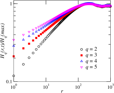
Figure 3: Generalized correlation function $H_{q}(r,t)$ calculated for $L=2000$ and $t=1000$. The data are averaged over $200$ independent runs and the error-bars are smaller than the symbol size.

The qth-order generalized height-height correlation function $H_{q}(r,t)$ (defined below) is commonly used in identifying multi-affine surfaces Barabási and Vicsek (1991); Barabasi and Stanley (1995).

$$H_{q}(r,t)=\{\langle\mid h(x+r,t)-h(x,t)\mid^{q}\rangle\}^{(1/q)},$$ (3)

The scaling properties of multi-affine surfaces can be described in terms of an infinite set of Hurst exponents Meakin (1998); Family and Vicsek (1991) $h_{q}$ which are obtained using,

$$H_{q}(r,t)\sim r^{h_{q}}.$$ (4)

For multi-affine interfaces, the exponents $h_{q}$ are known to vary with $q$ Meakin (1998). In Fig. 3, we plot the generalized correlation function $H_{q}(r,t)$ using $q$ = $2$, $3$, $4$, and $5$ for $G$ = $10$ at deposition time $t$ = $10^{3}$. For smaller $r$, we observe a power-law dependence of $H_{q}(r,t)$ on $r$ in accordance to Eq. (4). The slopes of the log-log plots shown in Fig. 3 depend on $q$ and indicate the presence of multi-scaling in the films generated by our VDP growth model.

III.2 Average Height and Growth Rate

The average height of the growth front $h_{avg}(t)$, is defined as,

$$h_{avg}(t)=\dfrac{1}{L}\sum_{x=1}^{L}h(x,t),$$ (5)

and quantifies the overall thickness of the film. Figure 4 shows the plot of $h_{avg}$ versus $t$ for different $G$ and $L=512$. For the studied values of $G$, the $h_{avg}$ versus $t$ plots show a linear relationship. This linear behavior is a consequence of restricting the growth to 1-D and the excluded volume constraint implemented in the growth process. In Fig. 4 with an increase in $G$, we observe a systematic increase in the slope of the $h_{avg}$ versus $t$ plot. We define the growth rate $R$ of the polymer film as,

$$R=\frac{dh_{avg}}{dt}.$$ (6)

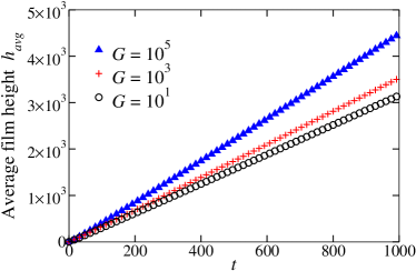
Figure 4: Variation of $h_{avg}$ as a function of deposition time $t$ for different $G$ and $L$ = 512. The data are averaged over 500 independent runs. The statistical errors are smaller than the symbol size.

In general one expects the polymer film’s growth rate to be proportional to the incoming free-monomer flux only, i.e. $R$ $\propto$ $F$ and it is natural to expect $R$ to be independent of $G(=D/F)$ since $F(=1/L)$ is a constant for a fixed $L$. However, in Fig. 4 our simulations show a strong dependence of $R$ on $G$ as well, and the growth rate $R$ is observed to increase monotonically with $G$. This $G$ dependent growth rate $R$ indicates that the growth rate is effected by monomer diffusion directly, i.e., there is a net uphill monomer diffusion current that is responsible for this $R-G$ relationship. We thus incorporate an additional term $r(G)$ that determines $R$ in addition to its dependence on $F$.

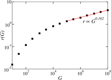
Figure 5: Variation of $r(G)$ as a function of $G$. The data were obtained for $L$ = $512$ and averaged over $500$ independent runs. The statistical errors are smaller than the symbol size.

$$R(G)=R_{0}+r(G),$$ (7)

where $R_{0}$ is the growth rate due to the random deposition flux only ($D$ = 0) and $r(G)$ is the growth rate induced only by the uphill diffusion of free-monomers. In Fig. 5 we show the variation of $r(G)$ as a function of $G$. We find a monotonic increase in $r(G)$ with an increase in $G$. This shows the strong influence of $G$ in determining the polymer film’s growth rate. Specifically, at higher $G$ we find $r(G)$ $\propto$ $G^{0.162(3)}$. This indicates that the growth rate due to uphill diffusion $r(G)$ asymptotically follows a power-law dependence with $G$.

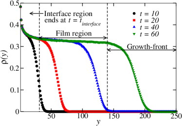
Figure 6: Lateral film density profiles $\rho\left(y\right)$ of polymer films grown on a $L=512$ substrate with $G=10$ at deposition times of $t=10$, $20$, $40$, and $60$ respectively. The statistical errors are smaller than the symbol size.

III.3 Characterization of the Kinetic Roughening

The morphology of the growth front can be characterized by studying its spatial and temporal evolution. In morphological scaling studies, typically two kinds of scaling behaviors are associated with the roughening kinetics: the global scaling and the local scaling Asikainen et al. (2002); Krug (1994); Ramasco et al. (2000). The growth models with anomalous kinetic roughening are known to have different scaling exponents in the local and the global scales. The local roughness exponents have been employed in studying the irregularly growing mound morphology and are often used in the experimental analysis Zhao et al. (2000); Jeffries et al. (1996). In general, the local roughness exponent $\alpha_{l}$ and the global roughness exponent $\alpha_{g}$ take different values depending on the type of scaling exhibited by the growth process. In the case of super-rough surfaces generated by nonequilibrium MBE growth models Das Sarma et al. (1994) and growth models with horizontal diffusion Amar et al. (1993), the assumption of the equivalence between the global and local descriptions of the surface is not valid and such behavior has been termed as anomalous scaling Das Sarma et al. (1994); Schroeder et al. (1993). The differences in the global and local scaling exponents have been attributed to the super-roughening and intrinsically anomalous spectrum observed in the anomalous scaling of surfaces López et al. (1997). For studying the morphological evolution of VDP generated polymer films, it is essential to identify their steady growth regime. To do so we employed the lateral film density $\rho\left(y\right)$ (at a height $y$ lattice units) of polymer film defined as,

$$\rho\left(y\right)=\frac{N\left(y\right)}{L},$$ (8)

where $N(y)$ represents the number of occupied lattice sites at a height y above the substrate. Calculations were performed on films with $L=512$, $G=10$ at deposition times of $t=10$, $20$, $40$, and $60$, respectively. Figure 6 shows the variation of $\rho(y)$ with $t$. Similar plots were obtained for other $G$ values also. Three distinct regions of the polymer film growth referred to as the interface region, the steady-state film region and the growth front were identified based on the Ref. Bowie and Zhao (2004). To evaluate the scaling exponents for kinetic roughening, we only concentrate on films with the deposition time $t\gg t_{interface}$.

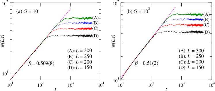
Figure 7: Time variation of the interface width $w(L,t)$ for (a) $G=10$ and (b) $G$ = $10^{3}$ with $L$ = $100$, $200$, and $300$. The data are averaged over $1.8\times 10^{3}$ independent runs.

III.3.1 Global Scaling Behavior

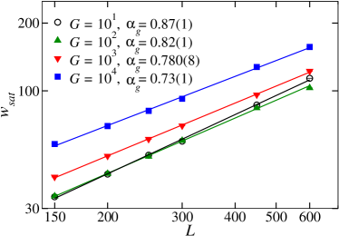
Figure 8: Variation of $w_{sat}$ with $L$ for $G$ varying from $10$ to $10^{4}$. The data are averaged over $1.8\times 10^{3}$ independent runs and the statistical errors are smaller than the symbol size.The error in the exponents were obtained from the curve-fit.

The global scaling of the growth front can be determined by studying the lattice size dependent interface width $w(L,t)$ defined as,

$$w(L,t)=\sqrt{\dfrac{1}{L}\sum_{i}^{L}\left[h(i)-h_{avg}\right]^{2}}.$$ (9)

In many 1-D morphological growth processes such as ballistic deposition Baiod et al. (1988); Family and Vicsek (1985), Eden model Family and Vicsek (1985), and solid-on-solid models Kim and Kosterlitz (1989), $w(L,t)$ usually follows the scaling law,

$$w(L,t)\sim t^{\beta}\qquad(t\ll t_{X}),$$ (10)

where exponent $\beta$ is known as the growth exponent that characterizes the time-dependence of surface roughening. For any given $L$, the power-law increase in $w(L,t)$ does

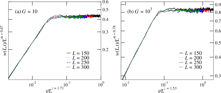
Figure 9: Rescaled plots of $w(L,t)/L^{\alpha_{g}}$ versus $t/L^{z_{g}}$. The “collapsed” curves shown in the plots are the scaling functions for (a) $G=10$, (b) $G=10^{3}$ and indicate the presence on dynamic scaling. The data are averaged over $1.8\times 10^{3}$ independent runs.

not continue indefinitely with $t$, and is followed by a saturation regime during which the $w(L,t)$ reaches a saturation value $w_{sat}$. The power-law growth regime and the saturation regime are separated by a crossover time $t_{X}$. As $L$ increases, $w_{sat}$ also follows a power-law Barabasi and Stanley (1995),

$$w(L,t)=w_{sat}\sim L^{\alpha_{g}}\qquad(t\gg t_{X}),$$ (11)

and ${\alpha_{g}}$ is referred to as the global roughness exponent Barabasi and Stanley (1995). The time $t_{X}$ at which the behavior of $w(L,t)$ crosses over from Eq. (10) to that of Eq. (11) depends on $L$ and scales as,

$$t_{X}\sim L^{z_{g}},$$ (12)

where $z_{g}$ is called the global dynamic exponent. Typically the scaling exponents are independent of specific interactions involved in the growth process and depend on the dimensionality and symmetries of the system Family and Vicsek (1985); Family (1986); Barabasi and Stanley (1995); Meakin (1998). For some growth processes, the exponents $\alpha_{g}$, $\beta$, and $z_{g}$ are unified using the dynamic scaling hypothesis Family and Vicsek (1985) (also known as the Family-Vicsek scaling) given as,

$$w(L,t)\sim L^{\alpha_{g}}\Psi\left(t/L^{z_{g}}\right),$$ (13)

where $\Psi\left(t/L^{z_{g}}\right)$ is referred to as the scaling function and satisfies,

$$\Psi\left(x\right)=\left\{\begin{array}[]{ll}x^{\beta}&\qquad\qquad\left(x\ll 1\right)\\ const&\qquad\qquad\left(x\gg 1\right),\\ \end{array}\right.$$ (14)

and

$$z_{g}=\alpha_{g}/\beta.$$ (15)

In Fig. 7 we show two representative plots of $w(L,t)$ versus $t$ on a log-log scale for (a) $G=10$, (b) $G=10^{3}$ and varying $L$. From both Figs. 7(a) and 7(b), for $t\ll t_{X}$, the $log(w(L,t))$ versus $log(t)$ shows a linear dependence implying a power-law behavior. For the same $G$ and $t\ll t_{X}$, the $w(L,t)$-$t$ plots overlap with one another for different $L$. We estimated $\beta$ by fitting Eq. (10) to the plots of $w(L,t)$ in Fig. 7 for the film region $t\ll t_{X}$. We obtained average $\beta=0.509(8)$ and $0.51(2)$ for $G$ = $10$ and $10^{3}$ respectively. For other $G$ values, the $\beta$ obtained was close to $0.50$ and we observed an invariance of $\beta$ (within the error-bars) with $G$. The statistical average and error bars in $\beta$ were obtained from $1.8\times 10^{3}$ independent simulations. The VDP model studied here is similar to the ballistic deposition model with additional degree of freedom including diffusion, polymer initiation, extension and merger. However, unlike the atomic diffusion in MBE growth, the free-monomer diffusion is confined by the linear geometry of the polymer chain. From Fig. 2 one can observe that in most cases the polymer chains are more or less perpendicular to the substrate. Since the free-monomers can only move along the polymer chain, most of the diffusion happens in vertical direction rather than in lateral direction (which is the case for MBE growth). Yet, the vertical diffusion does not contribute significantly to extra roughness increasing or decreasing (the total particle number should be conserved) in the growth front due to the porous nature of the film as compared to the random deposition model. Thus, it is expected that the growth exponent will be close to that of random deposition $(\beta\approx 0.50)$. We calculated $w_{sat}$ by averaging $w(L,t)$ for $t\gg t_{X}$ from the data shown in Figs. 7(a) and 7(b). Figure 8 shows the plot of $w_{sat}$ versus $L$ on the log-log scale for $G$ varying from $10$ to $10^{4}$. The exponent $\alpha_{g}$ was estimated for each $G$ using Eq. (11). With an increase in $G$ from $10$ to $10^{4}$, $\alpha_{g}$ was found to decrease from $0.87(1)$ to $0.73(1)$, the error-bars in $\alpha_{g}$ were obtained from the curve fitting. The exponent $\alpha_{g}$ is known to be closely related to the surface fractal dimension Barabasi and Stanley (1995). The smaller the $\alpha_{g}$, the larger is the fractal dimension. Our observation of a decrease in $\alpha_{g}$ with an increase in $G$ shows that the fractal dimension of the growth front increases with $G$, i.e. there are more spatial frequency fluctuations in the film morphology with an increase in $G$. This finding is consistent with the growth front profiles shown in Fig. 2. This result also demonstrates that $G$ induces a large effective vertical growth rate $R(G)$ (shown in Fig. 5) and the large $R(G)$ in turn produces a much rougher film surface.
To determine whether the VDP process obeys the dynamic scaling behavior, we start with an assumption that VDP growth follows the dynamic scaling hypothesis and obtain $z_{g}$ through Eq. (15). As $w(L,t)$ scales with both $t$ (Eq. (10)) and $L$ (Eq. (11)) we can rescale the $w(L,t)$ curve shown in Fig. 7 by plotting $w/L^{\alpha_{g}}$ versus $t/L^{z_{g}}$ to see whether those curves “collapse”. For $G=10$ we obtain $\alpha_{g}$ = $0.87(1)$, $\beta$ = $0.509(8)$ and according to Eq. (15) $z_{g}$ = $1.71(1)$ and for $G=10^{3}$ we get $\alpha_{g}$ = $0.780(8)$, $\beta$ = $0.51(2)$, and $z_{g}$ = $1.53(2)$. We use the data from Figs. 7(a) and 7(b) and divide $w(L,t)$ by $L^{\alpha_{g}}$. This shifts the curves of varying $L$ vertically on the log-log scale. According to Eq. (11), these curves now saturate at the same value of the ordinate $w/L^{\alpha_{g}}$, however their saturation times do not overlap. We then rescale the time axis and plot $t/L^{z_{g}}$ for both cases of $G$. This rescaling of time axis according to Eq. (12) leads to a horizontal shift of the curves and the curves now saturate at the same abscissa $t/L^{z_{g}}$. In Figs. 9(a) and 9(b) we show the rescaled plots of $w(L,t)$ for $G=10$, $10^{3}$ and consequently observe the “collapse” of individual curves for varying $L$ onto a single curve. This characteristic “collapsed” curve shown in Figs. 9(a) and 9(b) is the scaling function $\Psi\left(t/L^{z_{g}}\right)$ mentioned in the Eq. (14). The scaling functions obtained in Figs. 9(a) and 9(b) are observed to follow Eq. (14) for both cases of $G=10$ and $10^{3}$. For other $G$ values, we observed similar “collapse” behavior indicating the global dynamic scaling of growth fronts of the polymer films grown using VDP.

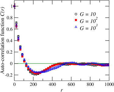
Figure 10: Auto-correlation function $C(r,t)$ calculated for $L=2000$ and $t=1000$ (averaged over $200$ independent runs).

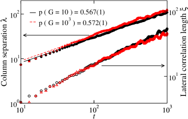
Figure 11: Estimates for column separation $\lambda$ and lateral correlation length $\xi$ obtained for $G=10(circles)$ and $G=10^{3}(triangles)$. Open symbols correspond to $\xi$ and filled symbols correspond to $\lambda$. The data are averaged over $200$ independent simulations with $L=2000$ and $t=1000$. The error in the exponents were obtained from the curve-fit.

III.3.2 Local Scaling Behavior

The local scaling behavior of the growth front can be understood from studying the spatial correlation functions: the auto-correlation function $C(r,t)$ and height-height correlation function $H(r,t)$ that describe the local properties of growing interfaces,

$$C(r,t)=\langle h(x+r,t)\cdot h(x,t)\rangle,$$ (16)

$$H(r,t)=\{\langle[h(x+r,t)-h(x,t)]^{2}\rangle\}=2[w^{2}-C(r,t)],$$ (17)

where $r$ is the translation distance also referred to as the lag or slip Zhao et al. (2001) and $\langle...\rangle$ denotes a spatial average over the entire system. The functions $C(r,t)$ and $H(r,t)$ are directly related as shown in Eq. (17) and differ only by a constant pre-factor of $2w^{2}$. The $H(r,t)$ scales in the same way as the interface width and is often used in studying the kinetic roughening Barabasi and Stanley (1995). In order to obtain

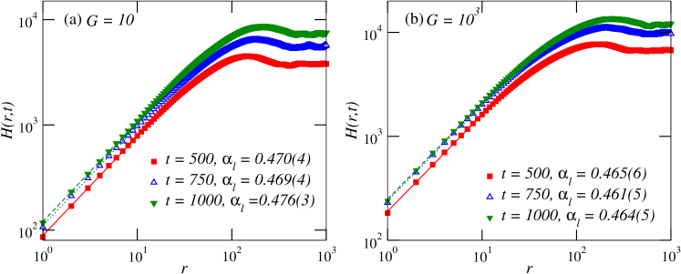
Figure 12: Height-height correlation function $H(r,t)$ for (a): $G=10$, (b): $G=10^{3}$ using $L=2000$ at $t$ = $500$, $750$, and $1000$. The data are averaged over $200$ independent runs and error in the exponents were obtained from the curve-fit.

accurate parameters from the correlation functions, it is important to account for the accuracy of statistical averages.

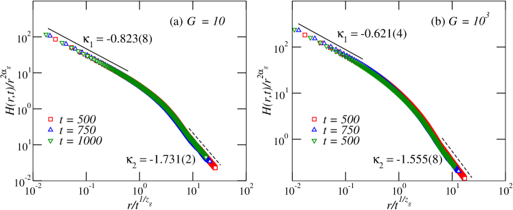
Figure 13: Plots of rescaled $H(r,t)$ showing the data collapse for (a): $G=10$, and (b): $G=10^{3}$ using $L=2000$ at $t$ = $500$, $750$, and $1000$. The data are averaged over $200$ independent runs and error in the exponents were obtained from the curve-fit. The straight lines are plotted as a guide to the eye. The scaling agrees with Eq. (21).

For the random Gaussian model surface studied by Ref. Zhao et al. (2001), converging $H(r,t)$ were obtained within an order of $\left(\xi/L\right)^{d/2}$ where $d$ is the system dimension and $\xi$ is the lateral correlation length. The accuracy depends not only on the number of data points, but also on the sample size. It is the ratio $\xi/L$, not the number of data points, that determines the accuracy. Once the ratio $\xi/L$ is known, one may not be able to increase the accuracy no matter how many data points are collected Zhao et al. (2001). This rule is different from the law of large numbers for independent random variables. This important difference needs to be recognized while studying spatially correlated systems. Ideally, one would like to have $\sqrt{\xi/L}\ll 1$, i.e, $L\rightarrow\infty$. However, due to the computational constraints we performed calculations using $L=2000$ and $t=1000$. For a random self-affine surface, $C(r,t)$ usually decays to zero with an increase in $r$. The shape of the decay depends on the type of the surface and the decay rate depends on the distance over which two points $x$, $x+r$ become uncorrelated. In Fig. 2 the polymer growth front does not appear to be a random rough surface, instead it has regular fluctuations of the columnar structures. Figure 10 shows the $C(r,t)$ for $L=2000$ after a deposition time $t=1000$ for $G=10$, $10^{2}$, and $10^{3}$ used to characterize the surface morphology as a function of $t$. We can define two different lateral length scales: the lateral correlation length $\xi$ and the average column-separation $\lambda$. The lateral correlation length $\xi$ defines a representative lateral dimension of a rough surface and is estimated through $C(r,t)$ using $C(r=\xi,t)=C(0,t)/e$. Within a distance of $\xi$ the surface heights of any two points are correlated. The parameter $\lambda$ characterizes a wavelength-selection of a surface and is determined by measuring the value of $r$ corresponding to the first zero-crossing of $C(r,t)$ Zhao et al. (2001). The variation of $\lambda$ with $t$ represents how the columnar structures coarsen with deposition time. In general, the evolution of the columnar feature size follows a power law with $t$ given by Yu and Amar (2002)

$$\lambda\propto t^{p},$$ (18)

and $p$ can be referred to as the coarsening exponent.

In Fig. 11 we plot $\lambda$ versus $t$ for $L=2000$ and $G=10$ and $10^{3}$ along with the estimates for $p$. With an increase in $G$ from $10$ to $10^{3}$, $p$ is found to remain close to $0.57$. The invariance of $p$ indicates that the coarsening of the columnar structures follow a power law that is unaffected by the ratio $G$. And we believe that this is dominated by the shadowing effect due to monomer vapor coming from all different angles uniformly.

The local roughness exponent ${\alpha_{l}}$ of the growth front can be obtained from $H(r,t)$ using Barabasi and Stanley (1995); Asikainen et al. (2002)

$$H(r,t)\sim r^{2\alpha_{l}}\qquad(r\ll\xi).$$ (19)

In Figs. 12(a) and 12(b) we plot $H(r,t)$ for $t=500$, $750$, and $1000$ along with the estimates for ${\alpha}_{l}$ for $L=2000$ and $G=10$, $10^{3}$ respectively. For a given $G$ and varying $t$, the estimates of ${\alpha_{l}}$ were observed to remain invariant within statistical-errors. From Figs. 12(a) and 12(b), we obtained an average ${\alpha_{l}}$ of $0.470(3)$ and $0.460(3)$ for $G=10$ and $10^{3}$ respectively. A comparison between $\alpha_{g}$ and $\alpha_{l}$ (shown in Fig. 8 and Fig. 12) shows $\alpha_{g}>\alpha_{l}$ for studied $G$ and the scaling behavior is observed to be different at short and large length scales. For small $r$, the plots of $H(r,t)$ do not overlap at varying coverage and show the presence of non-stationary anomalous scaling Meakin (1998). The vertical temporal shift in the $H(r,t)$ observed in Fig 12 is due to the difference between $\alpha_{g}$ and $\alpha_{l}$ and indicates the presence of anomalous scaling. The mechanisms that lead to anomalous scaling can be separated into two classes: super-roughening $({\alpha}_{g}>1)$ and intrinsic anomalous scaling López and Rodríguez (1996); López et al. (1997); Ramasco et al. (2000). The anomalous growth exponent ${\beta}_{\ast}=({\alpha}_{g}-{\alpha}_{l})/z_{g}$ López et al. (1997) measures the difference between $\alpha_{g}$, $\alpha_{l}$ and can be obtained from the scaling of $H(r,t)$ López et al. (1997)

$$H(r,t)=r^{2\alpha_{g}}g_{A}(r/t^{1/z_{g}}),$$ (20)

and the anomalous scaling function $g_{A}(u)$ López et al. (1997, 1997) satisfies

$$g_{A}(u)\sim\left\{\begin{array}[]{ll}u^{-{\kappa}_{1}}&\qquad\qquad\left(u\ll 1\right)\\ u^{-{\kappa}_{2}}&\qquad\qquad\left(u\gg 1\right)\\ \end{array}\right.$$ (21)

$${\kappa}_{1}=2({\alpha}_{g}-{\alpha}_{l})\\$$ (22)

$${\kappa}_{2}=2{\alpha_{g}}.$$ (23)

In Figs. 13(a) and 13(b) we show the plots of ${H(r,t)}/r^{2\alpha_{g}}$ versus $r/t^{1/z_{g}}$ and obtain the “data-collapse” for $G=10$ and $10^{3}$ respectively. The “collapsed” curves shown in Figs. 13(a) and 13(b) are the scaling functions $g_{A}(u)$ (for $G=10$ and $10^{3}$) mentioned in Eq. (20). For both $G$, the scaling functions obtained in Fig. 13 satisfy Eq. (21) in accordance with the theory for anomalous scaling López et al. (1997, 1997). The exponents $\kappa_{1}$ and $\kappa_{2}$ were obtained from $g_{A}(u)$ plots using Eq. (21). For $G=10$ we have $\kappa_{1}=0.823(8)$, $\kappa_{2}=1.731(2)$ and for $G=10^{3}$ we obtained $\kappa_{1}=0.621(4)$, $\kappa_{2}=1.555(8)$. For both $G$, we find that the exponents $\kappa_{1}$ and $\kappa_{2}$ obtained from the curve-fit satisfy Eqs. (22) and (23) for the numerical estimates of $\alpha_{g}$ and $\alpha_{l}$ obtained from Eq. (11) and Eq. (19).

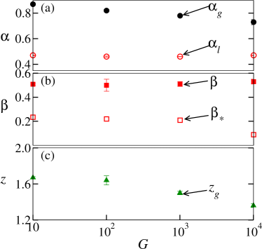
Figure 14: Variation of exponents $\alpha_{g}$, $\beta$, $z_{g}$, ${\alpha_{l}}$, and ${\beta}_{\ast}$ with $G$. The global exponents were calculated after $t=5000$ and the data were averaged over $1.8\times 10^{3}$ independent runs. The local exponents were calculated using $L=2000$ and $t=1000$. The data were averaged over $200$ runs and the error in the exponents were obtained from the curve-fit.

The dynamic scaling exponents of the kinetic roughening are summarized in Figs. 14(a), 14(b), and 14(c) which shows the variation of global scaling exponents $\alpha_{g}$, $\beta$, $z_{g}$ and local exponents $\alpha_{l}$, ${\beta}_{\ast}$ with $G$. With an increase in $G$ from $10$ to $10^{4}$, we found $\beta\approx 0.50$, $\alpha_{g}$ decreased from $0.87(1)$ to $0.73(1)$, and $z_{g}$ decreased from $1.71(1)$ to $1.38(2)$. On the local length scale, an increase in $G$ did not effect a noticeable change in $\alpha_{l}$ $(\alpha_{l}\approx 0.46)$ and ${\beta}_{\ast}$ was observed to decrease from $0.23(4)$ to $0.18(8)$.

IV Conclusions

We have performed 1+1D Monte Carlo simulation of VDP growth process by considering free-monomer deposition, free-monomer diffusion, polymer initiation, extension and polymer merger. The ratio $G$ of the free-monomer diffusion coefficient $D$ to the deposition rate $F$ was found to have a strong influence on the film’s growth morphology. The growth rate $R(G)$ of the polymer film was found to increase monotonically with an increase in $G$. This is due to the consequence of an upper diffusion flux of free-monomers. The detailed analysis of the surface morphology indicated the presence of very different scaling behavior at global and local length scales. The kinetic roughening study of film interface indicates anomalous scaling and multiscaling. With an increase in $G$ from $10$ to $10^{4}$, the global growth exponent $\beta\approx 0.50$ was found to be invariant, whereas the global roughness exponent $\alpha_{g}$ decreased from $0.87(1)$ to $0.73(1)$ along with a corresponding decrease in the global dynamic exponent $z_{g}$ from $1.71(1)$ to $1.38(2)$. The global scaling exponents were found to follow the dynamic scaling hypothesis with $z_{g}=\alpha_{g}/\beta$ for various $G$. With an increase in $G$ from $10$ to $10^{4}$, the average local roughness exponent $\alpha_{l}$ remained close to $0.46$ with ${\alpha_{l}}\neq\alpha_{g}$, this observation is unlike the ones obtained in self-affine surfaces Family and Vicsek (1991); Barabasi and Stanley (1995). The anomalous growth exponent ${\beta}_{\ast}$ was also found to decrease from $0.23(4)$ to $0.18(8)$ with an increase in $G$. Even though our model is in 1+1D as compared to the 2+1D experiments, our estimates of $\alpha_{l}$ and ${\beta}_{\ast}$ are close to the experimental findings of $\alpha\approx 0.5$ to $0.7$ and $\beta=0.25\pm 0.03$ obtained from the AFM studies of linear PA-N films grown by VDP Zhao et al. (2000); Strel’tsov et al. (2008). The similarity between the experimental and simulational estimates appears to be a coincidence since the dimension of the two systems are totally different. We also did not observe the changes in the dynamic roughening behavior reported by Ref. Lee et al. (2008), perhaps due to the limitations of our current simulation model in considering the effect of free-monomer diffusion only. This makes us believe that the kinetic roughening of the polymer films is sensitive to the specific molecular-level interactions, relaxations of polymer chains through inter-polymer interactions, and the intrinsic nature of polymerization process that need to be accounted for in the future simulations.

V ACKNOWLEDGEMENTS

ST and DPL were partially supported by the NSF grant DMR-0810223. ST and YPZ were also partially supported by NSF grant CMMI-0824728. ST would like to thank S. J. Mitchell for help with the visualization tools.

References

- Lu and Moore (1997) T.-M. Lu and J. A. Moore, Mater. Res. Soc. Bull 20, 28 and references therein (1997).
- Wong (1993) C. P. Wong, Polymers for Electronic and Photonic Application (Academic Press, Boston, MA, 1993).
- Gorham (1966) W. F. Gorham, Journal of Polymer Science Part A-1: Polymer Chemistry 4, 3027 (1966).
- Lahann et al. (2003) J. Lahann, M. Balcells, H. Lu, T. Rodon, K. F. Jensen, and R. Langer, Analytical Chemistry 75, 2117 (2003).
- Szulczewski et al. (2000) G. J. Szulczewski, T. D. Selby, K.-Y. Kim, J. D. Hassenzahl, and S. C. Blackstock, in The 46th International Symposium of the American Vacuum Society (2000), vol. 18, pp. 1875–1880.
- Usui (1998) H. Usui, in Proceedings of 1998 International Symposium on Electrical Insulating Materials (1998), pp. 577–582.
- Biederman et al. (2003) H. Biederman, V. Stelmashuk, I. Kholodkov, A. Choukourov, and D. Slavnsk, Surface and Coatings Technology 174, 27 (2003).
- Chrisey and Hubler (1994) D. B. Chrisey and G. K. Hubler, eds., Pulsed Laser Deposition of Thin Films (Wiley-Interscience, 1994).
- Piqu et al. (2003) A. Piqu, R. C. Y. Auyeung, J. L. Stepnowski, D. W. Weir, C. B. Arnold, R. A. McGill, and D. B. Chrisey, Surface and Coatings Technology 163, 293 (2003).
- Schreiber (2004) F. Schreiber, Physica Status Solidi Applied Research 201, 1037 (2004).
- Collins et al. (1994) G. W. Collins, S. A. Letts, E. M. Fearon, R. L. McEachern, and T. P. Bernat, Phys. Rev. Lett. 73, 708 (1994).
- Biscarini et al. (1997) F. Biscarini, P. Samor’i, O. Greco, and R. Zamboni, Phys. Rev. Lett. 78, 2389 (1997).
- Fortin and Lu (2002) J. Fortin and T. Lu, Chemistry of Materials 14, 1945 (2002).
- Mattox (1998) D. M. Mattox, Handbook of Physical Vapor Deposition (PVD) Processing (Noyes Publications, Berkshire, UK, 1998).
- Barabasi and Stanley (1995) A.-L. Barabasi and H. E. Stanley, Fractal Concepts in Surface Growth (Cambridge University Press, Cambridge, England, 1995).
- Meakin (1998) P. Meakin, Fractals, scaling, and growth far from equilibrium (Cambridge University Press, Cambridge, England, 1998).
- Pal and Landau (1994) S. Pal and D. P. Landau, Phys. Rev. B 49, 10597 (1994).
- Shim et al. (1998) Y. Shim, D. P. Landau, and S. Pal, Phys. Rev. E 58, 7571 (1998).
- Zhao et al. (1999a) Y.-P. Zhao, A. R. Hopper, G.-C. Wang, and T.-M. Lu, Phys. Rev. E 60, 4310 (1999a).
- Bowie and Zhao (2004) W. Bowie and Y. P. Zhao, Surface Science 563, L245 (2004).
- Zhao et al. (2000) Y.-P. Zhao, J. B. Fortin, G. Bonvallet, G.-C. Wang, and T.-M. Lu, Phys. Rev. Lett. 85, 3229 (2000).
- Aue and De Hosson (1997) J. Aue and J. T. M. De Hosson, Applied Physics Letters 71, 1347 (1997).
- Lee et al. (2008) I. J. Lee, M. Yun, S.-M. Lee, and J.-Y. Kim, Phys. Rev. B 78, 115427 (2008).
- Lai and Das Sarma (1991) Z.-W. Lai and S. Das Sarma, Phys. Rev. Lett. 66, 2348 (1991).
- Marsaglia (2003) G. Marsaglia, J. Mod. Appl. Statist. Methods 2, 2 (2003).
- Yu and Amar (2002) J. Yu and J. G. Amar, Phys. Rev. E 66, 021603 (2002).
- Drotar et al. (2000) J. T. Drotar, Y.-P. Zhao, T.-M. Lu, and G.-C. Wang, Phys. Rev. B 62, 2118 (2000).
- Beach (1977) W. F. Beach, Macromolecules 11, 72 (1977).
- Amar et al. (1994) J. G. Amar, F. Family, and P.-M. Lam, Phys. Rev. B 50, 8781 (1994).
- Karunasiri et al. (1989) R. P. U. Karunasiri, R. Bruinsma, and J. Rudnick, Phys. Rev. Lett. 62, 788 (1989).
- Bales and Zangwill (1989) G. S. Bales and A. Zangwill, Phys. Rev. Lett. 63, 692 (1989).
- Zhao et al. (1999b) Y.-P. Zhao, J. T. Drotar, G.-C. Wang, and T.-M. Lu, Phys. Rev. Lett. 82, 4882 (1999b).
- Drotar et al. (2001) J. T. Drotar, Y.-P. Zhao, T.-M. Lu, and G.-C. Wang, Phys. Rev. B 64, 125411 (2001).
- Barabási and Vicsek (1991) A.-L. Barabási and T. Vicsek, Phys. Rev. A 44, 2730 (1991).
- Family and Vicsek (1991) F. Family and T. Vicsek, eds., Dynamics of Fractal Surfaces (World Scientific, Singapore, 1991).
- Asikainen et al. (2002) J. Asikainen, S. Majaniemi, M. Dubé, J. Heinonen, and T. Ala-Nissila, Eur. Phys. J. B 30 (2002).
- Krug (1994) J. Krug, Phys. Rev. Lett. 72, 2907 (1994).
- Ramasco et al. (2000) J. J. Ramasco, J. M. López, and M. A. Rodríguez, Phys. Rev. Lett. 84, 2199 (2000).
- Jeffries et al. (1996) J. H. Jeffries, J.-K. Zuo, and M. M. Craig, Phys. Rev. Lett. 76, 4931 (1996).
- Das Sarma et al. (1994) S. Das Sarma, S. V. Ghaisas, and J. M. Kim, Phys. Rev. E 49, 122 (1994).
- Amar et al. (1993) J. G. Amar, P.-M. Lam, and F. Family, Phys. Rev. E 47, 3242 (1993).
- Schroeder et al. (1993) M. Schroeder, M. Siegert, D. E. Wolf, J. D. Shore, and M. Plischke, Europhys. Lett. 24, 563 (1993).
- López et al. (1997) J. M. López, M. A. Rodríguez, and R. Cuerno, Phys. Rev. E 56, 3993 (1997).
- Baiod et al. (1988) R. Baiod, D. Kessler, P. Ramanlal, L. Sander, and R. Savit, Phys. Rev. A 38, 3672 (1988).
- Family and Vicsek (1985) F. Family and T. Vicsek, Journal of Physics A 18, L75 (1985).
- Kim and Kosterlitz (1989) J. M. Kim and J. M. Kosterlitz, Phys. Rev. Lett. 62, 2289 (1989).
- Family (1986) F. Family, Journal of Physics A 19, L441 (1986).
- Zhao et al. (2001) Y. Zhao, G.-C. Wang, and T.-M. Lu, Characterization of amorphous and crystalline rough surface : principles and application (Academic Press, San Diego, CA, 2001).
- López and Rodríguez (1996) J. M. López and M. A. Rodríguez, Phys. Rev. E 54, R2189 (1996).
- López et al. (1997) J. M. López, M. A. Rodríguez, and R. Cuerno, Physica A: Statistical and Theoretical Physics 246, 329 (1997).
- Strel’tsov et al. (2008) D. R. Strel’tsov, A. I. Buzin, E. I. Grigor’ev, P. V. Dmitryakov, K. A. Mailyan, A. V. Pebalk, and S. N. Chvalun, Nanotechnologies in Russia 3, 494 (2008).