Local estimation of the Hurst index of multifractional Brownian motion by Increment Ratio Statistic method

Abstract

We investigate here the Central Limit Theorem of the Increment Ratio Statistic of a multifractional Brownian motion, leading to a CLT for the time varying Hurst index. The proofs are quite simple relying on Breuer-Major theorems and an original freezing of time strategy. A simulation study shows the goodness of fit of this estimator.

Keywords: Increment Ratio Statistic, fractional Brownian motion, local estimation, multifractional Brownian motion, wavelet series representation.

Introduction

The aim of this paper is a simple proof of Central Limit Theorem (CLT in all the sequel) for the convergence of Increment Ratio Statistic method (IRS in all the sequel) to a time varying Hurst index.

Hurst index is the main parameter of fractional Brownian motion (fBm in all the sequel), it belongs to the interval $(0,1)$ and it will be denote by $H$ in all the following. For fBm, the Hurst index drives both path roughness, self-similarity and long memory properties of the process. FBm was introduced by Kolmogorov [20] as Gaussian "spirals" in Hilbert space and then popularized by Mandelbrot & Van Ness [22] for its relevance in many applications. However, during the two last decades, new devices have allowed access to large then huge datatsets. This put in light that fBm itself is a theoretical model and that in real life situation the Hurst index is, at least, time varying. This model, called multifractional Brownian motion (mBm) has been introduced, independently by Lévy-Véhel & Peltier [21] and Benassi et al [9]. Other generalizations of fBm remain possible, for e.g. Gaussian processes with a Hurst index depending of the scale, so-called multiscale fBm [5], when $H$ is piecewise constant as in the Step Fractional Brownian Motion see [3], or a wide range of Gaussian or non-Gaussian processes fitted to applications (see for example [14, 4]). However, for simplicity of the presentation, in this work we restrict ourselves to mBm.

In statistical applications, we estimate the time varying Hurst index through a CLT. Actually, CLT provides us confidence intervals. Different statistics can be used to estimate the Hurst index. Among the popular methods, let us mention quadratic variations, generalized quadratic variations, see [8, 15, 16], and wavelet analysis, see e.g [1] or [6]. Above methods can be expansive in term of time complexity. For this reason, Surgailis et al [27] and Bardet & Surgailis [7] have proposed a new statistic named increment ratio which can be used for estimating the Hurst index $H$ and is faster than the wavelet or the quadratic variations methods, at the price of a slightly larger variance.

CLT for the different estimators of Hurst index are presently standard in the case of fBm, but became very technical in the case of mBm. The main novelty of our work is the simplicity of the proofs. In our point of view, mBm is a fBm where the constant Hurst index $H$ has been replaced by time varying Hurst index. It is well known that the random field $(H,t)\mapsto B(H,t)$ is irregular with respect to time $t$, actually with regularity $H$ which belongs to $(0,1)$. It is less kown that this field is infinitely differentiable with respect to $H$, see Meyer-Sellan-Taqqu (1999) and Ayache and Taqqu (2005). Thus, for all time $t_{0}$, we can freeze the time varying Hurst index, and the mBm behaves approximatively like a fBm. Eventually, CLT for mBm follows from CLT for fBm combined with a control of "freezing error". This new and natural technology allows us to go further and obtain for example a CLT for the Hurst function evaluated at a finite collection of times and also quantitative convergence speed in the CLT. Note that, up to our knowledge, the "freezing Hust index" strategy for estimation in mBm was introduced, without further proof, in Bertrand et al [10].

The remainder of this paper is organized as follows. In Section 1, we recall a definition of fBm and the definition of the Increment Ration Statistic. Next, in section 2, we review definitions of fBm and mBm and precise the localization procedure (or freezing). The main result is stated in Section 3 and some numerical simulations are presented in Section 4. All technical proofs are postponed in Section 5.

1 Recall on fBm and Increment Ratio Statistic

In this section, we present the Increment Ratio Statistic (IRS) method obtained by filtering centered Gaussian processes with stationary increments. Before, we recall definition of the processes under consideration.

1.1 Definition of fBm and Gaussian processes with stationary increments

We describe fBm through its harmonizable representation. However, it is simpler to adopt a more general framework and then specify fBm as a particular case. Let $X=\left(X(t),t\in[0,1]\right)$ be a zero mean Gaussian process with stationary increments, the spectral representation theorem (see Cramèr and Leadbetter [18] or Yaglom [28]), asserts that the following representation is in force

$$X(t) = \int_{\mathbb{R}}(1-e^{it\xi})\cdot f^{1/2}(\xi)\;dW(\xi),\leavevmode\nobreak\ \leavevmode\nobreak\ \leavevmode\nobreak\ \leavevmode\nobreak\ \mbox{for all}\leavevmode\nobreak\ \leavevmode\nobreak\ t\in[0,1],$$

where $W(dx)$ is a Wiener measure with adapted real and imaginary part such that $X(t)$ is real valued for all $t$. The function $f$ is a Borelian even, positive and is called spectral density of $X$. To insure convergence of the stochastic integral, $f$ should satisfies the condition given by

$$\int_{R}\big{(}1\wedge|\xi|^{2}\big{)}\cdot f(\xi)\;d\xi<\infty.$$ (1)

Example: Fractional Brownian motion with Hurst parameter $H\in(0,1)$ and scale parameter $\sigma>0$ corresponds to a spectral density given by

$$f(\xi)=\sigma^{2}|\xi|^{-(2H+1)}\text{ for all }\xi\in\mathbb{R}.$$ (2)

In this paper, we denote fBm by $B(H,t)$ when $\sigma=1$. Stress that this choice is not the conventional one. But, IRS is homogeneous and does not depends on a multiplicative factor. Thus, in sake of simplicity, we can impose the extra condition $\sigma=1$.

1.2 Definition of the $a$-Generalized increments

In all the sequel, we consider the observation of the process $X$ at discrete regularly spaced times, that is the observation of $\left(X(t_{0}),\ldots,X(t_{n})\right)$ at times $t_{k}=k/n$. Secondly, we consider a filter denoted by $a$ of length $L+1$ and of order $p\geq 1$, where $p\leq L$ are two integers. It corresponds to an arbitrary finite fixed real sequence $a:=(a_{0},\ldots,a_{L})\in\mathbb{R}^{L+1}$ having $p$ vanishing moments, i.e.,

$$\sum_{l=0}^{L}a_{l}l^{i}=\left\{\begin{array}[]{ll}\displaystyle 0&\mbox{if }i\in\{0,\ldots,p-1\}\\ \displaystyle\sum_{l=0}^{L}a_{l}l^{p}\neq 0&\mbox{if }i=p.\\ \end{array}\right.$$ (5)

Consequently, it is easy to prove, for any integer $m$, that

$$\sum_{l_{1}=0}^{L}\sum_{l_{2}=0}^{L}a_{l_{1}}a_{l_{2}}\left|l_{1}-l_{2}\right|^{m}=\left\{\begin{array}[]{ll}\displaystyle 0&\mbox{if }m\in\{0,\ldots,2p-1\}\\ \displaystyle\left(\sum_{l=0}^{L}a_{l}l^{p}\right)^{2}\neq 0&\mbox{if }m=2p.\\ \end{array}\right.$$ (8)

The family of such filters will be denotes $\mathcal{A}(p,L)$. Then, the $a$-Generalized increments of the discrete process $\left(X(t_{k})\right)_{0\leq k\leq n}$ are defined, for all $0\leq k\leq n-L-1$, as follows

$$\Delta_{a}X(t_{k})=\sum_{k=0}^{L}a_{l}X(t_{k+l})$$ (9)

and their harmonizable representations are given by

$$\Delta_{a}X(t_{k})=\int_{\mathbb{R}}e^{it_{k}\xi}g_{a}(-\xi/n)f^{1/2}(\xi)\;dW(\xi)$$

where $g_{a}(\cdot)$ is specified as follows

$$g_{a}(u):=\sum_{l=0}^{L}a_{l}e^{ilu}.$$ (10)

Examples: In the simple case where $a:=(a_{0}=1,a_{1}=-1)$, the operator $\Delta_{a}$ corresponds to a discrete increment of order 1, and when $a:=(a_{0}=1,a_{1}=-2,a_{2}=1)$, the operator $\Delta_{a}$ represents the second order differences.

1.3 Definition of the Increment Ratio Statistic

Let $\left(\Delta_{a}X(t_{k})\right)_{0\leq k\leq n-L-1}$ be the $a$-Generalized increments sequence defined by $\eqref{delta:tk}$ from the discrete observation $\left(X(t_{k})\right)_{0\leq k\leq n}$. Then, the IRS introduced by Bardet and Surgailis [7] is given by

$$\mbox{IRS}_{a,n}(X)=\frac{1}{n-L}\sum_{k=0}^{n-L-1}\psi\left(\Delta_{a}X(t_{k}),\Delta_{a}X(t_{k+1})\right)$$ (11)

where $\psi(\cdot,\cdot)$ is described as follows

$$\psi(x,y):=\left\{\begin{array}[]{ll}\displaystyle\frac{\left|x+y\right|}{\left|x\right|+\left|y\right|}&\mbox{if }(x,y)\in\mathbb{R}^{2}\backslash\{(0,0)\}\\ \displaystyle\ 1&\mbox{if }(x,y)=(0,0).\\ \end{array}\right.$$

IRS of fractional Brownian motion

In the case of the fBm with Hurst parameter $H\in\left(0,1\right)$, i.e $X(t)=B_{H}(t)$, Bardet and Surgailis have established in [7, Corollary 4.3, p.13], under some semi-parametric assumptions, the following CLT for the statistics $\mbox{IRS}_{a,n}$

$$\sqrt{n}\left(\mbox{IRS}_{a,n}(B_{H})-\Lambda_{a}(H)\right)\begin{array}[t]{c}\stackrel{{\scriptstyle{\cal D}}}{{\rightarrow}}\\ {}\hfil\end{array}\mathcal{N}(0,\Sigma^{2}_{a}(H))\text{ with }\left\{\begin{array}[]{ll}\ H\in\left(0,3/4\right)&\mbox{if }a=(1,-1)\\ \ H\in\left(0,1\right)&\mbox{if }a=(1,-2,1)\\ \end{array}\right.$$ (17)

where the sign $\begin{array}[t]{c}\stackrel{{\scriptstyle{\cal D}}}{{\rightarrow}}\\ {}\hfil\end{array}$ means convergence in distribution,

$$\Lambda_{a}(H) := \Lambda_{0}\left(\rho_{a}(H)\right)$$ (18)

$$\Lambda_{0}(r) := \frac{1}{\pi}\arccos(-r)+\frac{1}{\pi}\sqrt{\frac{1+r}{1-r}}\log\left(\frac{2}{1+r}\right)$$ (19)

$$\rho_{a}(H) = \left\{\begin{array}[]{ll}\displaystyle 2^{2H-1}-1&\mbox{if }a=(1,-1)\\ \displaystyle\frac{-3^{2H}+2^{2H+2}-7}{8-2^{2H+1}}&\mbox{if }a=(1,-2,1)\\ \end{array}\right.$$ (22)

and the asymptotic variance $\Sigma^{2}_{a}(H)$ is given by

$$\Sigma^{2}_{a}(H)=\sum_{j\in\mathbb{Z}}\mbox{cov}\left(\psi\left(\Delta_{a}B_{H}(t_{0}),\Delta_{a}B_{H}(t_{1})\right),\psi\left(\Delta_{a}B_{H}(t_{j}),\Delta_{a}B_{H}(t_{j+1})\right)\right).$$

The graphs of $\Lambda_{0}(\rho),\rho_{a}(H)$ and $\Lambda_{a}(H)$, with $a=(1,-1)\text{ or }a=(1,-2,1)$, are given in Figure 1, Figure 2 and Figure 3 below.

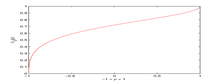
Figure 1: The graph of $\Lambda_{0}(\rho)$.

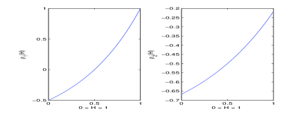
Figure 2: The graphs of $\rho_{a}(H)$ with $a=(-1,1)$(left) and $a=(1,-2,1)$ (right).

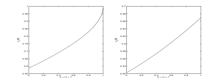
Figure 3: The graphs of $\Lambda_{a}(H)$ with $a=(-1,1)$(left) and $a=(1,-2,1)$ (right).

It is easy to prove that the function $H\mapsto\Lambda_{a}(H)$, with $a=(1,-2,1)$, is a monotonic increasing function in the interval (0,1), see Figure 3. Therefore, $\displaystyle\widehat{H}_{n}=\Lambda^{-1}_{a}\left(\mbox{IRS}_{a,n}(B_{H})\right)$ provides an estimator of the Hurst parameter $H$ with convergence rate $\mathcal{O}\left(\sqrt{n}\right)$. Moreover, we refer to Stoncelis and Vaičiulis [26] for a numerical approximation of the variance $\Sigma^{2}_{a}(H)$ with $a=(1,-1)\text{ or }a=(1,-2,1)$, needed for construction of confidence intervals, see [7, Corollary 4.3, p.13 and Appendix, p.32].

2 Going from fBm to mBm and return by freezing

The main goal of this section is to present different representations for the FBm and the mBm enabling us to present the time freezing strategy we will use to prove our main theorems.

FBm and its different representations

Fractional Brownian motion was introduced by Kolmogorov [20] and then made popular by Mandelbrot & Van Ness [22]. This process has been widely used in applications to model data that exhibit self-similarity, stationarity of increments, and long range dependence. FBm with Hurst parameter $H\in(0,1)$, denoted by $\left(B_{H}(t),t\in[0,1]\right)$, is a centered Gaussian process with covariance function defined for $s,t\in[0,1]$ by

$$\mathbb{E}\left[B_{H}(t)B_{H}(s)\right]=\frac{1}{2}\left(t^{2H}+s^{2H}+|t-s|^{2H}\right).$$ (23)

This process is characterized by its Hurst index which drives both pathwise regularity, self-similarity and long memory, see e.g. the overview in Bertrand et al (2010). Before going further, let us precise notations: in all the sequel we will denote by $B_{H}$ the fBm and $B(H,t)$ the random field depending on both Hurst index and time. Up to a multiplicative constant the two notions coincide, more precisely we have $B_{H}(t)=C(H)\times B(H,t)$ for $C(H)$ a non-negative constant depending on $H$.

Fractional Brownian motion, $\left(B_{H}(t),t\in[0,1]\right)$, can be represented through its harmonizable representation (1.1, 2), or its moving-average representation (see Samorodnitsky & Taqqu [25, Chapter 14]). A third representation is the wavelet series expansion introduced by Meyer et al [23], and then nicely used by Ayache and Taqqu (2003 and 2005). In this case, it is judicious to shift to the random field representation defined as follows

$$B(H,t) = \sum_{j\in Z}\sum_{k\in{\bf Z}}a_{jk}(t,H)\,\epsilon_{jk},\leavevmode\nobreak\ \leavevmode\nobreak\ \leavevmode\nobreak\ \leavevmode\nobreak\ \mbox{for all}\leavevmode\nobreak\ \leavevmode\nobreak\ t\in[0,1]$$ (24)

where $(\epsilon_{jk})_{(j,k)\in Z^{2}}$ is a sequence of standard Gaussian random variables $\mathcal{N}(0,1)$, the non-random coefficients $a_{jk}(t,H)$ are given by $\displaystyle a_{jk}(t,H)=\int_{\mathbb{R}}(1-e^{it\xi})\cdot|\xi|^{-(H+1/2)}\widehat{\psi}_{j,k}(\xi)\;d\xi$, and $\widehat{\psi}_{j,k}$ is the Fourier transform of the Lemarié-Meyer wavelet basis $\psi_{j,k}$. Let us refer to Ayache and Taqqu (2003) for all the technical details. To put it into a nutshell, by using the Meyer et al ’s Lemma ([23]), we can prove the existence of an almost sure event $\Omega^{*}$, that is such that $\Pr(\Omega^{*})=1$, such that for all $\omega\in\Omega^{*}$ the series (24 ) converges uniformly for $(H,t)\in K$ where $K$ is any compact subset of $(0,1)\times\mathbb{R}$. Moreover, the field is infinitively differentiable with respect to $H$ with derivatives bounded uniformly on every compact subset of $(0,1)\times\mathbb{R}$ by a constant $C^{*}(\omega)>0$ where $C^{*}$ is a positive random variable with finite moments of every order.

MBm and its different representations

To be short, mBm is obtained by plugging a time varying Hurst index $t\mapsto H(t)$ into one of the three representations of the fBm given above, that is the moving average representation, the harmonizable one ((1.1, 2)) or the wavelet series expansion (24 ). The function $t\mapsto H(t)$ should be at least continuous, and if the Hölder regularity of the function $t\mapsto H(t)$ is greater than $\max(H(t),t\in[0,1])$ (the so-called condition $\bf(\mathcal{C})$ in Ayache and Taqqu (2003)), then for every time $t\in[0,1]$ the roughness of mBm is given by $H(t)$. Les us also refer to Cohen [17] where he proves that the moving average representation and the harmonizable representation of mBm are equivalent up to a multiplicative deterministic function, and to Meyer et al. to the almost sure equality of harmonizable representation and wavelet series expansion.

With this tools, we are now in order to precise our "freezing" technology:

MBm behaves locally as a fBm

By applying Taylor expansion of order 1 around any fixed time $t^{*}\in[0,1]$, we obtain the following formula

$$B(H(t),t)\mathbb{I}_{\Omega^{*}} = B(H^{*},t)\mathbb{I}_{\Omega^{*}}+R(t)\mathbb{I}_{\Omega^{*}}$$ (25)

where $R(t)$ refers to the Taylor rest which satisfies

$$\sup_{s\in[0,1]}\left|R(s)\mathbb{I}_{\Omega^{*}}\right|\leq C^{*}(\omega)|H(t)-H^{*}|$$ (26)

with $C^{*}>0$ a positive random variable with finite moments of every order. Noting that $H^{*}$ corresponds to the value of the Hurst function $H(\cdot)$ at $t^{*}$, i.e., $H^{*}=H(t^{*})$ and $\mathbb{I}_{\Omega^{*}}$ represents the indicator function of a subset $\Omega^{*}$ defined by: $\mathbb{I}_{\Omega^{*}}(\omega)=\left\{\begin{array}[]{ll}\ 1&\mbox{if }\omega\in\Omega^{*}\\ \ 0&\mbox{else }\end{array}\right.$. Next, if we know that the Hurst function $H(\cdot)$ has a Hölder regularity of order $\eta>0$, so we obtain immediately that

$$\sup_{s\in[0,1]}\left|R(s)\mathbb{I}_{\Omega^{*}}\right|\leq M^{*}\,\mathbb{I}_{\Omega^{*}}\,|t-t^{*}|^{\eta}$$ (27)

with $M^{*}=c\times C^{*}>0$ a positive random variable with finite moments of every order.

3 Main results

This section is dedicated to the CLT of the IRS localized version for the mBm. Let us however first give a simple result on the CLT for the IRS of Gaussian processes with stationary increments, which, applied to the fractional Brownian motion, gives with a simple proof the result of Bardet-Surgailis [7].

We thus consider a process $X$ observed through the knowledge of $\left(X(t_{0}),\ldots,X(t_{n})\right)$ with $t_{k}=k/n$ for $k=1,\dots,n$. The corresponding increment ratio statistic $\mbox{IRS}_{a,n}(X)$ is defined by $\eqref{IRSgaus}$, with a filter $a\in\mathcal{A}(p,L)$, that is satisfying $\eqref{filter}$.

Theorem 1 (Fractional Brownian motion)

• Let $X$ be a zero mean Gaussian process with stationary increments. We assume that

  $$\sum_{j\in\mathbb{Z}}|r_{a}(j)|^{2}<+\infty$$ (28)

  where $r_{a}(j):=\mbox{cov}\left(\Delta_{a}X(t_{0}),\Delta_{a}X(t_{j})\right)$ for $j\in\mathbb{Z}$ is supposed independent of $n$. Then

  $$\sqrt{n}\left(\mbox{IRS}_{a,n}(X)-\Lambda_{0}(\rho_{a})\right) \begin{array}[t]{c}\stackrel{{\scriptstyle{\cal D}}}{{\rightarrow}}\\ {}\hfil\end{array} \mathcal{N}(0,\Sigma^{2}_{a})$$ (31)

  where $\Lambda_{0}(\cdot)$ is defined by $\eqref{L0}$, $\rho_{a}$ represents the correlation between two successive $a$-Generalized increments, and the asymptotic variance $\Sigma^{2}_{a}$ is given by

  $$\Sigma^{2}_{a}:=\sum_{j\in\mathbb{Z}}\mbox{cov}\left(\psi\left(\Delta_{a}X(t_{0}),\Delta_{a}X(t_{1})\right),\psi\left(\Delta_{a}X(t_{j}),\Delta_{a}X(t_{j+1})\right)\right)$$

  and is well defined and belongs to $[0,+\infty)$.

• In particular, let $X$ be a fBm, that is $X=B_{H}$ with Hurst parameter $H\in\left(0,1\right)$. Moreover, in the case $p=1$ assume the extra assumption $\ H\in\left(0,3/4\right)$. Then CLT (31) is in force where $\Lambda_{a}(\cdot)=\Lambda_{0}(\rho_{a}(\cdot))$ is a monotonic increasing function of $H$ with $\Lambda_{0}(\cdot)$, resp. $\rho_{a}(\cdot)$ described by $\eqref{L0}$, resp. $\eqref{rho_aH}$, and the asymptotic variance $\Sigma^{2}_{a}$ is given by

  $$\Sigma^{2}_{a}:=\sum_{j\in\mathbb{Z}}\mbox{cov}\left(\psi\left(\Delta_{a}B_{H}(t_{0}),\Delta_{a}B_{H}(t_{1})\right),\psi\left(\Delta_{a}B_{H}(t_{j}),\Delta_{a}B_{H}(t_{j+1})\right)\right)$$

  which is well defined and belongs to $[0,+\infty)$. $\square$

Remark:

1. In the sequel, in order to could inverse function $\Lambda_{a}(\cdot)$, we will assume that the filter $a\in\mathcal{A}(p,L)$ satisfy $L=p\geq 1$ and $a_{l}=(-1)^{p-l}\binom{p}{l}$ for all $l\in\{0,\ldots,p\}$. The class of such filters will be denoted $\mathcal{B}(p)$ and named binomial filters. This restriction is motivated by the fact that in the particular case where $a\in\mathcal{B}(p)$, the correlation function $\rho_{a}(\cdot)$ defined by $\eqref{rho_aH}$, is a monotonic increasing function of $H$, instead of in the general case where $a\in\mathcal{A}(p,L)$ it is not always true.

2. The regularity of $\Lambda_{a}(H)$ enables us then to get via the well known Delta-method the CLT for the Hurst parameter. However no closed formulae for $\Lambda_{a}(H)^{-1}$ is available so that the limiting covariance will be no further explicit.

3. We stress once again that the proof of the theorem is quite simple. Note also that using recent results of Nourdin et al [24, Th. 2.2], we even have that there exists a sequence $\gamma(n)$ decaying to zero such that for all $h\in C^{2}$ and $N\sim\mathcal{N}(0,\Sigma^{2}_{a})$

   $$\left|\mathbb{E}\left[h\left(\sqrt{n}\left(\mbox{IRS}_{a,n}(X)-\Lambda_{0}(\rho_{a})\right)\right)-h(N)\right]\right|\leq\|h^{\prime\prime}\|_{\infty}\,\gamma(n).$$

   The precise estimation of $\gamma(n)$ is however out of the scope of the present paper and will be found in [19]. Using [24, Cor. 2.4], we also have that the previous CLT may be reinforced to a convergence in 1-Wasserstein distance or in Kolmogorov distance.

4. The reader will have noticed that the assumption $r_{a}(j):=\mbox{cov}\left(\Delta_{a}X(t_{0}),\Delta_{a}X(t_{j})\right)$ independent of $n$ for all $j\in\mathbb{Z}$ is a quite strong one. Indeed, for the multiscale Brownian motion, this not true. However, in a sense, it is asymptotically true and it may then be applied to prove the convergence of the IRS to the Hurst parameter related to the highest frequency. See [19] for further details.

To achieve our final goal, we state by presenting a Lemma where we prove that the localized version of IRS for mBm converges in $L^{2}(\Omega)$ to the IRS of fBm with a certain rate.

Localized version of the IRS for multifractional Brownian motion

Let us consider a multifractional Brownian motion with Hurst function $H(\cdot)$ denoted by $X=\left(B(H(t),t),t\in[0,1]\right)$. Secondly, let $t^{*}\in(0,1)$ be an arbitrary fixed point, then we denote by $\nu_{n}\left(\gamma,t^{*}\right)$ the set of indices around $t^{*}$, given by

$$\nu_{n}\left(\gamma,t^{*}\right) = \{k\in\{0,\ldots,n-L-1\}:|t_{k}-t^{*}|\leq n^{-\gamma}\}$$ (32)

$$= \{\lfloor nt^{*}-n^{1-\gamma}\rfloor,\ldots,\lfloor nt^{*}+n^{1-\gamma}\rfloor\}$$ (33)

where $\lfloor x\rfloor$ is the integer part of $x$ and $\gamma\in(0,1)$ is a fixed parameter which allows to control the size of $\nu_{n}\left(\gamma,t^{*}\right)$ which cardinal is equal to $v_{n}(\gamma):=2n^{1-\gamma}+1$. Finally, for any $n$ large enough, we denote by $\mbox{IRS}_{a,n}^{\gamma,t^{*}}\left(B_{H(\cdot)}\right)$ the localized version of IRS defined as follows

$$\mbox{IRS}_{a,n}^{\gamma,t^{*}}\left(B_{H(\cdot)}\right) = \frac{1}{2n^{1-\gamma}+1}\sum_{k=\lfloor nt^{*}-n^{1-\gamma}\rfloor}^{\lfloor nt^{*}+n^{1-\gamma}\rfloor}\psi\left(\Delta_{a}B_{H(t_{k})}(t_{k}),\Delta_{a}B_{H(t_{k+1})}(t_{k+1})\right).$$ (34)

With these notations, we are in order to state our main result:

Theorem 2 (Multifractional Brownian motion)

• Let $X$ be a mBm, its localized IRS be defined by (34) and assume that $\gamma(1+\eta)>1$. Then

  $$n^{(1-\gamma)/2}\left(\mbox{IRS}_{a,n}^{\gamma,t^{*}}\left(B_{H(\cdot)}\right)-\Lambda_{a}(H^{*})\right)\begin{array}[t]{c}\stackrel{{\scriptstyle{\cal D}}}{{\rightarrow}}\\ {}\hfil\end{array}\mathcal{N}(0,\Sigma^{2}_{a})\text{ with }\left\{\begin{array}[]{ll}\ H^{*}\in\left(0,3/4\right)&\mbox{if }p=1\\ \ H^{*}\in\left(0,1\right)&\mbox{if }p\geq 2\\ \end{array}\right.$$ (39)

  where $\Lambda_{a}(\cdot)=\Lambda_{0}(\rho_{a}(\cdot))$ is a monotonic increasing function of $H^{*}$ with $\Lambda_{0}(\cdot)$ & $\rho_{a}(\cdot)$ described by $\eqref{L0}$ & $\eqref{rho_aH}$, and the asymptotic variance $\Sigma^{2}_{a}$ is given by

  $$\Sigma^{2}_{a}:=\sum_{j\in\mathbb{Z}}\mbox{cov}\left(\psi\left(\Delta_{a}B_{H^{*}}(t_{0}),\Delta_{a}B_{H^{*}}(t_{1})\right),\psi\left(\Delta_{a}B_{H^{*}}(t_{j}),\Delta_{a}B_{H^{*}}(t_{j+1})\right)\right)$$

  and is well defined and belongs to $[0,+\infty)$.

• Let now consider $0<t_{0}<t_{1}<...<t_{m}$ for a finite $m$ then under the same assumption we can enhance the previous CLT to the vector

  $$n^{(1-\gamma)/2}\left(\mbox{IRS}_{a,n}^{\gamma,t_{1}}\left(B_{H(\cdot)}\right)-\Lambda_{a}(H(t_{1})),...,\mbox{IRS}_{a,n}^{\gamma,t_{m}}\left(B_{H(\cdot)}\right)-\Lambda_{a}(H(t_{m}))\right)$$

  with a well defined limiting covariance $\mathfrak{S}$. $\square$

Remark:

1. Here again, one can use results of [24] to get explicit estimates on the speed of convergence for this CLT.

2. It is highly interesting to upgrade the previous CLT to the trajectory level, needing then a tightness result, for example to test if the Hurst coefficient is always greater than 1/2, or to perform other test. Such kind of result will be developed in [19].

4 Numerical results

In this section, for numerical estimation of the Hurst index by IRS, one has chosen a binomial filter of order 2, i.e. $a=(1,-2,1)$, insuring the convergence of the estimator $\widehat{H}_{n}$ for any $H\in(0,1)$. At first, we analyze through Monte-Carlo simulations the efficiency of the Hurst parameter of fBm estimator given by IRS. Then, we study the estimators of some Hurst functions of mBm obtained by localized version of IRS, and we compare it with the estimators given by Generalized Quadratic Variations (GQV) method, see e.g Coeurjolly [16].

Estimation of the Hurst index of fBm

At first, by using Wood and Chan [13] algorithm, for $n=10000$ we have simulated three replications of the fBm sequences $B_{H}=\left(B_{H}(t_{0}),\ldots,B_{H}(t_{n})\right)$, at regularly spaced times such that $t_{k}=k/n$ with $k=0,\ldots,n$ , for three values of the Hurst parameter $H$, denoted $\{H_{1},H_{2},H_{3}\}$, and given by

$\mathbf{(\mathcal{C}_{1})}$

$H_{1}=0.3<1/2$ for short range dependent case,

$\mathbf{(\mathcal{C}_{2})}$

$H_{2}=1/2$ for standard Brownian motion,

$\mathbf{(\mathcal{C}_{3})}$

$H_{3}=0.7>1/2$ for long range dependent case,

see Figure 4 below.

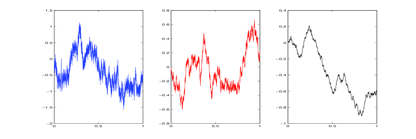
Figure 4: Simulated fBm process with $H=0.3$ (left), $H=0.5$ (middle) and $H=0.7$ (right).

Then, for each sample $\mathbf{(\mathcal{C}_{i})}$ with $i\in[1,3]$, we have computed the increment ratio statistic $IRS_{2,n}(B_{H_{i}})$ and estimated the Hurst index given by $\displaystyle\widehat{H}_{n,i}=\Lambda^{-1}_{2}\left(\mbox{IRS}_{2,n}(B_{H_{i}})\right)$. We remark that the IRS methods provide good results given in Table 1 below.

Exact values of $H$	0.3	0.5	0.7
Estimated values of $H$	0.3009	0.4993	0.7000

Table 1: Estimated values of $H$.

These examples are plainly confirmed by Monte Carlo simulations. Indeed, for each case $\mathbf{(\mathcal{C}_{i})}$ with $i\in[1,3]$, we have made $M=1000$ simulations of independent copies of fBm sequences $B^{(k)}_{H_{i}}=\left(B^{(k)}_{H_{i}}(t_{0}),\ldots,B^{(k)}_{H_{i}}(t_{n})\right)$, for $k=1,\ldots,M$. We find also good results illustrated by the following histograms, see Figure 5, which represent the distribution of the estimator $\widehat{H}_{n,i}$, for $i\in[1,3]$. Thus, we have computed the standard deviation $\mathbb{E}|\widehat{H}-H|^{2}$ given in Table 2 below.

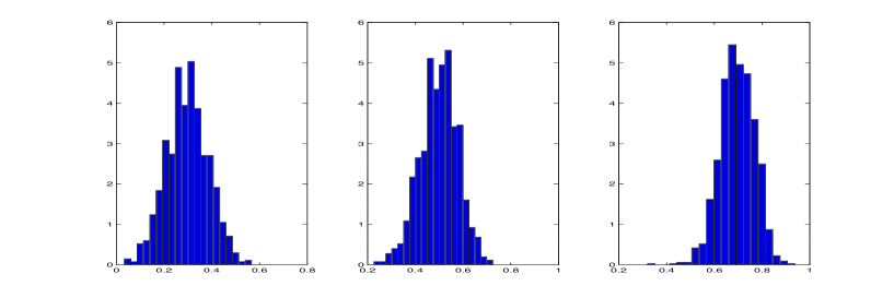
Figure 5: Distribution of the estimated values of $H$ in the case $H=0.3$ (left), $H=0.5$ (middle) and $H=0.7$ (right).

Different values of $H$	0.3	0.5	0.7
Standard deviation	$8.1865\times 10^{-5}$	$7.6914\times 10^{-5}$	$6.9837\times 10^{-5}$

Table 2: Standard deviation.

Local estimation of the Hurst function of mBm

To synthesis a sample path of a mBm, one has used the Wood and Chan circulant matrix improved with kriging interpolation method, which is faster than Cholesky-Levinson factorization algorithm. In fact, both methods are not exact but provide good results. For, $n=10000$, we have simulated three samples of the mBm sequences $B_{H(\cdot)}=\left(B_{H(t_{0})}(t_{0}),\ldots,B_{H(t_{n})}(t_{n})\right)$, at regularly spaced times such that $t_{k}=k/n$ with $k=0,\ldots,n$ , for three types of the Hurst function $H(\cdot)$, namely

$\mathbf{(\mathcal{C}_{4})}$

Linear function: $H_{4}(t)=0.1+0.8t$,

$\mathbf{(\mathcal{C}_{5})}$

Periodic function $H_{5}(t)=0.5+0.3\sin(\pi t)$,

$\mathbf{(\mathcal{C}_{6})}$

Logistic function: $\displaystyle H_{6}(t)=0.3+\frac{0.3}{(1+\exp(-100(t-0.7)))}$,

see Figure 6 below.

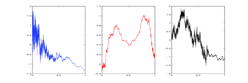
Figure 6: Simulated mBm process with $H(\cdot)$ linear function (left), $H(\cdot)$ periodic function (middle) and $H(\cdot)$ logistic function (right).

Then, for each sample $\mathbf{(\mathcal{C}_{i})}$ with $i\in[4,6]$, we have estimated the Hurst function $\widehat{H}_{n,i}$ by using the localized version of IRS with $\gamma=0.3$ and the GQV method. We note that both methods provide correct results represented by Figure 7 below.

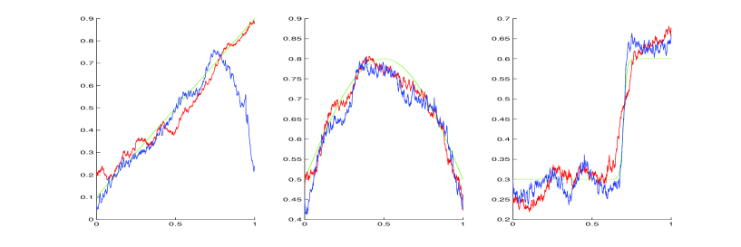
Figure 7: Estimation of the Hurst function $H(\cdot)$ with $H(\cdot)$ linear function (left), $H(\cdot)$ periodic function (middle) and $H(\cdot)$ logistic function (right). The graphs of function $H(\cdot)$, $\widehat{H}_{n}^{(IRS)}(\cdot)$ its estimation by IRS, and $\widehat{H}_{n}^{(GQV)}(\cdot)$ its estimation by GQV, are represented in green, red and blue respectively.

These results are plainly confirmed by Monte Carlo simulations. Actually, for each case $\mathbf{(\mathcal{C}_{i})}$ with $i\in[4,6]$, we have made $M=1000$ simulations of independent copies of mBm sequences $B^{(k)}_{H_{i}(\cdot)}=\left(B^{(k)}_{H_{i}(t_{0})}(t_{0}),\ldots,B^{(k)}_{H_{i}(t_{n})}(t_{n})\right)$, for $k=1,\ldots,M$. Then we have computed the Mean Integrate Square Error (MISE) defined as $\displaystyle\text{MISE}=\mathbb{E}\left(\frac{1}{n+1}\sum_{j=0}^{n}\left|\widehat{H}(t_{j})-H(t_{j})\right|^{2}\right)=\mathbb{E}\|\widehat{H}-H\|_{L^{2}(0,1)}^{2}$ which is a criterion widely used in functional estimation, see Table 3 below.

	$H(\cdot)$ Linear	$H(\cdot)$ Periodic	$H(\cdot)$ Logistic
MISE by IRS	$2.6743\times 10^{-4}$	$1.4743\times 10^{-4}$	$5.3546\times 10^{-3}$
MISE by GQV	$8.9547\times 10^{-4}$	$5.4743\times 10^{-4}$	$8.9743\times 10^{-4}$

Table 3: MISE given by IRS method and GQV method

We observe through Table 3 that both methods provide globally the same results when the function $H(\cdot)$ varies slowly (see linear and periodic cases), whereas in the case where $H(\cdot)$ presents the abrupt variation it appears that the GQV is a bit more precise compared to the IRS method.

5 Proofs of the main results

This section contains the proof of the results of Section 3. Note that we have divided the proof of Theorem 1 in two parts: first we consider the general case of Gaussian processes with stationary increments and then in a second part we investigate the application to fractional Bronwnian motion.

5.1 Proof of localization

First, we can deduce as a corollary that the $a$-Generalized increments sequence $\left(\Delta_{a}X(t_{k})\right)_{0\leq k\leq n-L-1}$ form a family of stationary identically distributed centered Gaussian r.v. with variance

$$\sigma^{2}_{a,n} = \mbox{cov}\left(\Delta_{a}X(t_{k}),\Delta_{a}X(t_{k})\right)$$

$$= \int_{\mathbb{R}}|g_{a}(\xi/n)|^{2}\cdot f(\xi)\;d\xi$$

$$= 2\int_{\mathbb{R}_{+}}|g_{a}(\xi/n)|^{2}\cdot f(\xi)\;d\xi,,$$

covariance given, for all $0\leq k_{1},k_{2}\leq n-L-1$, by

$$\mbox{cov}_{a,n}(t_{k_{1}},t_{k_{2}}) = \mbox{cov}\left(\Delta_{a}X(t_{k_{1}}),\Delta_{a}X(t_{k_{2}})\right)$$

$$= \int_{\mathbb{R}}e^{i(k_{1}-k_{2})\xi/n}|g_{a}(\xi/n)|^{2}\cdot f(\xi)\;d\xi$$

$$= 2\int_{\mathbb{R}_{+}}\cos\left((k_{1}-k_{2})\xi/n\right)|g_{a}(\xi/n)|^{2}\cdot f(\xi)\;d\xi,$$

and correlation between two successive $a$-Generalized increments defined by

$$\rho_{a,n}=\frac{\mbox{cov}\left(\Delta_{a}X(t_{k+1}),\Delta_{a}X(t_{k})\right)}{\left[\mbox{cov}\left(\Delta_{a}X(t_{k+1}),\Delta_{p}X(t_{k+1})\right)\right]^{1/2}\cdot\left[\mbox{cov}\left(\Delta_{a}X(t_{k}),\Delta_{p}X(t_{k})\right)\right]^{1/2}}=\frac{\mbox{cov}_{a,n}(t_{k+1},t_{k})}{\sigma^{2}_{a,n}},$$

where $g_{a}(\cdot)$ is described by $\eqref{g_a}$. Therefore, for a fixed $0\leq k\leq n-L-1$, it is easy to remark that there exist two independent standard Gaussian r.v. $Z_{k},Z_{k+1}\begin{array}[t]{c}\stackrel{{\scriptstyle{\cal D}}}{{\sim}}\\ {}\hfil\end{array}\mathcal{N}(0,1)$ such that

$$\Delta_{a}X(t_{k}) = \sigma_{a,n}Z_{k}$$ (40)

$$\Delta_{a}X(t_{k+1}) = \sigma_{a,n}\left(\rho_{a,n}Z_{k}+\sqrt{1-\rho^{2}_{a,n}}Z_{k+1}\right),$$ (41)

where the sign $\begin{array}[t]{c}\stackrel{{\scriptstyle{\cal D}}}{{\sim}}\\ {}\hfil\end{array}$ means equal in distribution.

Remark: In the particular case of the fBm, the correlation between two successive $a$-Generalized increments, $\rho_{a,n}$, does not depend on $n$. Indeed, we know that the spectral density of the fBm is given by $\eqref{densiteSpec}$, then we have

$$\rho_{a,n}(H)=\frac{\int_{\mathbb{R}_{+}}\cos(\xi/n)|g_{a}(\xi/n)|^{2}\cdot\xi^{-(2H+1)}\;d\xi}{\int_{\mathbb{R}_{+}}|g_{a}(\xi/n)|^{2}\cdot\xi^{-(2H+1)}\;d\xi}.$$

And after, we can change variable $\xi/n$ to $u$. So this implies that

$$\rho_{a,n}=\frac{\int_{\mathbb{R}_{+}}\cos(u)|g_{a}(u)|^{2}\cdot u^{-(2H+1)}\;du}{\int_{\mathbb{R}_{+}}|g_{a}(u)|^{2}\cdot u^{-(2H+1)}\;du}=\rho_{a}(H),$$

which is independent of $n$.

5.2 Proof of CLT for Gaussian Processes with stationary increments

The proof uses the notion of Hermite rank and Breuer-Major theorem, see for e.g Arcones [2, Theorem 4, p.2256] or Nourdin et al [24, Theorem 1, p.2].

Definition 1 (Hermite rank)

Let $G$ be a $\mathbb{R}^{d}$ Gaussian vector and $\phi:\mathbb{R}^{d}\rightarrow\mathbb{R}$ be a measurable function such that $\displaystyle\mathbb{E}\left|\phi(G)\right|^{2}<+\infty$. Then, the function $\phi$ is said to have Hermite rank equal to the integer $q\geq 1$ with respect to Gaussian vector $G$, if (a) $\displaystyle\mathbb{E}\left[\left(\phi(G)-\mathbb{E}\left(\phi(G)\right)\right)P_{m}(G)\right]=0$ for every polynomial $P_{m}$ $\left(\text{on }\mathbb{R}^{d}\right)$ of degree $m\leq q-1$; and (b) there exists a polynomial $P_{q}$ $\left(\text{on }\mathbb{R}^{d}\right)$ of degree $q$ such that $\displaystyle\mathbb{E}\left[\left(\phi(G)-\mathbb{E}\left(\phi(G)\right)\right)P_{q}(G)\right]\neq 0$.

We first give the proof of Theorem 1 in the general case of Gaussian processes with stationary increments and then in a separate part the application to fractional Brownian motion.

Proof of Theorem 1

First, in the sequel we denote by $G=\left(G_{k},G_{k+1}\right)=\left(\Delta_{a}X(t_{k}),\Delta_{a}X(t_{k+1})\right)$ these two successive stationary $a$-Generalized increments defined by $(\eqref{d1},\eqref{d2})$. Then, according to Bardet and Surgailis [7, Appendix, p.31], we know that

$$\mathbb{E}\left[\psi\left(G_{k},G_{k+1}\right)\right]=\Lambda_{0}(\rho_{a}), \mathbb{E}\left|\psi\left(G_{k},G_{k+1}\right)\right|^{2}<+\infty,$$ and

where $\Lambda_{0}(.)$ is defined by $\eqref{L0}$ and $\rho_{a}$ is the correlation between $G_{k}$ and $G_{k+1}$. To achieve our goal, we start by defining a new function $\phi:R^{2}\rightarrow\mathbb{R}$ such that

$$\phi(X,Y)=\psi(X,Y)-\Lambda_{0}(\rho_{a}).$$

Then, $\phi$ is in fact a Hermite function with respect to Gaussian vector $G=\left(G_{k},G_{k+1}\right)$ with rank equal to 2. Therefore, by applying Breuer-Major theorem, see e.g Arcones [2, Theorem 4, p.2256] or Nourdin et al [24, Theorem 1, p.2], we get directly the CLT $\eqref{TCLGauss}$. So, the key argument of our proof is to determine the Hermite rank of $\phi$. We include here the proof of the fact that the Hermite rank is 2 as the proof does not seem to appear elsewhere. Let $P_{0}(X,Y)=c_{0},P_{1}(X,Y)=c_{11}X+c_{12}Y+c_{10}$ and $P_{2}(X,Y)=X^{2}$ be three polynomials (on $\mathbb{R}^{2}$) with degree respectively 0, 1 and 2. First, it is easy to see that $\displaystyle\mathbb{E}\left[\phi(G)P_{0}(G)\right]=0$. Now, we must to show that $\displaystyle\mathbb{E}\left[\phi(G)P_{1}(G)\right]=0$. We have

$$\mathbb{E}\left[\phi(G)P_{1}(G)\right]=c_{11}\mathbb{E}\left[\phi(G)G_{k}\right]+c_{12}\mathbb{E}\left[\phi(G)G_{k+1}\right]+c_{10}\underbrace{\mathbb{E}\left[\phi(G)\right]}_{=0}.$$

Then,

$$\mathbb{E}\left[\phi(G)P_{1}(G)\right]=c_{11}\mathbb{E}\left[\psi(G_{k},G_{k+1})G_{k}\right]-c_{11}\Lambda_{0}(\rho_{a})\underbrace{\mathbb{E}[G_{k}]}_{=0}+c_{12}\mathbb{E}\left[\psi(G_{k},G_{k+1})G_{k+1}\right]-c_{12}\Lambda_{0}(\rho_{a})\underbrace{\mathbb{E}[G_{k+1}]}_{=0},$$

because $G_{k}$ and $G_{k+1}$ are zero-mean r.v. and due to the fact that the r.v $G_{k}$ and $G_{k+1}$ have a symmetric function, we can write without any restrictions that

$$\mathbb{E}\left[\phi(G)P_{1}(G)\right]=(c_{11}+c_{12})\mathbb{E}\left[\psi(G_{k},G_{k+1})G_{k}\right].$$

By using definition of $\left(G_{k},G_{k+1}\right)=\left(\Delta_{a}X(t_{k}),\Delta_{a}X(t_{k+1})\right)$ given by $(\eqref{d1},\eqref{d2})$, we get

$$(c_{11}+c_{12})^{-1}\mathbb{E}\left[\phi(G)P_{1}(G)\right]=\sigma_{a}\mathbb{E}\left[\psi\left(\sigma_{a}Z_{k},\sigma_{a}\left(\rho_{a}Z_{k}+\sqrt{1-\rho_{a}^{2}}Z_{k+1}\right)\right)Z_{k}\right]$$

where $Z_{k}$ and $Z_{k+1}$ are two independent standard Gaussian r.v. $Z_{k},Z_{k+1}\begin{array}[t]{c}\stackrel{{\scriptstyle{\cal D}}}{{\sim}}\\ {}\hfil\end{array}\mathcal{N}(0,1)$. Thus, by using homogeneity property of $\psi(\cdot,\cdot)$ specified by: $\psi(aX,aY)=\psi(X,Y)$, we obtain

$$(c_{11}+c_{12})^{-1}\mathbb{E}\left[\phi(G)P_{1}(G)\right]=\sigma_{a}\mathbb{E}\left[\psi\left(Z_{k},\left(\rho_{a}Z_{k}+\sqrt{1-\rho_{a}^{2}}Z_{k+1}\right)\right)Z_{k}\right].$$

Next, we have

$$(c_{11}+c_{12})^{-1}\mathbb{E}\left[\phi(G)P_{1}(G)\right]=\frac{\sigma_{a,n}}{2\pi}\int_{\mathbb{R}^{2}}\psi\left(z_{1},\rho_{a}z_{1}+\sqrt{1-\rho_{a}^{2}}z_{2}\right)z_{1}\exp\left(-\frac{z_{1}^{2}+z_{2}^{2}}{2}\right)dz_{1}dz_{2}.$$

And after, we can change variables $(z_{1},z_{2})$ to polar coordinates $(r\cos(\theta),r\sin(\theta))$. So, this implies that

$$2\pi\sigma_{p}^{-1}(c_{11}+c_{12})^{-1}\mathbb{E}\left[\phi(G)P_{1}(G)\right] = \int_{-\pi}^{\pi}\psi\left(\cos(\theta),\rho_{a}\cos(\theta)+\sqrt{1-\rho_{a}^{2}}\sin(\theta)\right)\cos(\theta)d\theta$$

$$\times \underbrace{\int_{0}^{+\infty}r^{2}\exp\left(-\frac{r^{2}}{2}\right)dr}_{=\sqrt{\pi/2}}.$$

Then, we remark that

$$\int_{-\pi}^{0}\psi\left(\cos(\theta),\rho_{a}\cos(\theta)+\sqrt{1-\rho_{a}^{2}}\sin(\theta)\right)\cos(\theta)d\theta =$$

$$\int_{-\pi}^{0}\frac{\left|\cos(\theta)+\rho_{a}\cos(\theta)+\sqrt{1-\rho_{a}^{2}}\sin(\theta)\right|}{\left|\cos(\theta)\right|+\left|\rho_{a}\cos(\theta)+\sqrt{1-\rho_{a}^{2}}\sin(\theta)\right|}\cos(\theta)d\theta \underbrace{=}_{u=\theta+\pi}$$

$$\int_{0}^{\pi}\frac{\left|\cos(u-\pi)+\rho_{a}\cos(u-\pi)+\sqrt{1-\rho_{a}^{2}}\sin(u-\pi)\right|}{\left|\cos(u-\pi)\right|+\left|\rho_{a}\cos(u-\pi)+\sqrt{1-\rho_{a}^{2}}\sin(u-\pi)\right|}\cos(u-\pi)du =$$

$$-\int_{0}^{\pi}\frac{\left|\cos(u)+\rho_{a}\cos(u)+\sqrt{1-\rho_{a}^{2}}\sin(u)\right|}{\left|\cos(u)\right|+\left|\rho_{a}\cos(u)+\sqrt{1-\rho_{a}^{2}}\sin(u)\right|}\cos(u)du =$$

$$-\int_{0}^{\pi}\psi\left(\cos(\theta),\rho_{a}\cos(\theta)+\sqrt{1-\rho_{a,n}^{2}}\sin(\theta)\right)\cos(\theta)d\theta.$$

Thus, we deduce directly that $\displaystyle\mathbb{E}\left[\phi(G)P_{1}(G)\right]=0$. In the similar way, it is easy to prove that $\displaystyle\mathbb{E}\left[\phi(G)P_{2}(G)\right]\neq 0$. So, by using Definition 1, we can say that $\phi$ is a Hermite function with rank equal to 2. Therefore, Theorem 1 becomes an application of Breuer-Major theorem which gives directly the proof of CLT $\eqref{TCLGauss}$. $\blacksquare$

Proof of CLT for FBm

Next, we present the correlation function properties of the $a$-Generalized increments sequence of a fBm.

Property 1 (Correlation function of the $a$-Generalized increments)

Let $\left(B_{H}(t),t\in[0,1]\right)$ be a fBm with Hurst parameter $H\in\left(0,1\right)$ and let $\left(\Delta_{a}B_{H}(t_{k})\right)_{0\leq k\leq n-L-1}$ its $a$-Generalized increments sequence defined by $\eqref{delta:tk}$, with $a\in\mathcal{A}(p,L)$ a filter given by $\eqref{filter}$. Then, for all $j\in\mathbb{Z}$, we have

$$r_{a,n}(j)=-\frac{1}{2\cdot n^{2H}}\times C_{a}(j)$$

where $r_{a,n}(j):=\mbox{cov}\left(\Delta_{a}B_{H}(t_{0}),\Delta_{a}B_{H}(t_{j})\right)$ and $C_{a}(j)$ is given by

$$C_{a}(j) := \sum_{l_{1},l_{2}=0}^{L}a_{l_{1}}a_{l_{2}}|j+l_{2}-l_{1}|^{2H}$$

$$\underset{j\rightarrow+\infty}{\sim} \binom{2H}{2p}\cdot\left(\sum_{l=0}^{L}a_{l}l^{p}\right)^{2}\times j^{2H-2p}\text{ with }\binom{2H}{2p}=\displaystyle\frac{\prod_{k=0}^{2p-1}(2H-k)}{(2p)!}.$$

And the correlation between two successive $a$-Generalized increments, is specified by

$$\rho_{a}(H)=\frac{\sum_{l_{1},l_{2}=0}^{L}a_{l_{1}}a_{l_{2}}|1+l_{2}-l_{1}|^{2H}}{\sum_{l_{1},l_{2}=0}^{L}a_{l_{1}}a_{l_{2}}|l_{2}-l_{1}|^{2H}}.$$ (42)

$\square$

Proof of Property 1

To compute the covariance function of the $a$-Generalized increments sequence, we start by using the initial formula of the covariance function of a fBm defined by $\eqref{covFBM}$. Then, we obtain

$$r_{a,n}(j) := \mbox{cov}\left(\Delta_{a}B_{H}(t_{0}),\Delta_{a}B_{H}(t_{j})\right)$$

$$= \sum_{l_{1},l_{2}=0}^{L}a_{l_{1}}a_{l_{2}}\mathbb{E}\left[B_{H}(t_{l_{1}})B_{H}(t_{j+l_{2}})\right]$$

$$= \frac{1}{2}\underbrace{\sum_{l_{1},l_{2}=0}^{L}a_{l_{1}}a_{l_{2}}t_{l_{1}}^{2H}}_{=0}+\frac{1}{2}\underbrace{\sum_{l_{1},l_{2}=0}^{L}a_{l_{1}}a_{l_{2}}t_{j+l_{2}}^{2H}}_{=0}-\frac{1}{2}\sum_{l_{1},l_{2}=0}^{L}a_{l_{1}}a_{l_{2}}|t_{j+l_{2}}-t_{l_{1}}|^{2H}$$

$$= -\frac{1}{2\cdot n^{2H}}\times C_{a}(j)$$

where $C_{a}(j)=\sum_{l_{1},l_{2}=0}^{L}a_{l_{1}}a_{l_{2}}|j+l_{2}-l_{1}|^{2H}$. Now, we give an equivalent of $C_{a}(j)$ when $j\rightarrow+\infty$. To do this, we use the Taylor expansion as follows

$$C_{a}(j) = j^{2H}\times\sum_{l_{1},l_{2}=0}^{L}a_{l_{1}}a_{l_{2}}\left|1+\frac{l_{1}-l_{2}}{j}\right|^{2H}$$

$$= j^{2H}\times\left[\underbrace{\sum_{l_{1},l_{2}=0}^{L}a_{l_{1}}a_{l_{2}}\cdot 1}_{=0}+\sum_{k=1}^{+\infty}\binom{2H}{k}j^{-k}\sum_{l_{1},l_{2}=0}^{L}a_{l_{1}}a_{l_{2}}|l_{2}-l_{1}|^{k}\right].$$

Next, by using $\eqref{doubleSum}$, we know that when we sum over $k$, every term in the expansion gives a zero contribution for any integer $k<2p$. So this implies that

$$C_{a}(j) = \binom{2H}{2p}\cdot\left(\sum_{l=0}^{L}a_{l}l^{p}\right)^{2}\times j^{2H-2p}+o\left(j^{2H-2p}\right)$$

$$\underset{j\rightarrow+\infty}{\sim} \binom{2H}{2p}\cdot\left(\sum_{l=0}^{L}a_{l}l^{p}\right)^{2}\times j^{2H-2p}.$$

This finishes the proof of Property 1. $\blacksquare$

And after, we note that the function $\psi(\cdot,\cdot)$ satisfies the homogeneity property specified by: $\psi(aX,aY)=\psi(X,Y)$. So, this allows us to rewrite $\mbox{IRS}_{a,n}(B_{H})$ as follows

$$\mbox{IRS}_{a,n}(B_{H})=\frac{1}{n-L}\sum_{k=0}^{n-L-1}\psi\left(\Delta_{a}B_{H}^{\text{std}}(t_{k}),\Delta_{a}B_{H}^{\text{std}}(t_{k+1})\right)$$

where $\Delta_{a}B_{H}^{\text{std}}$ represents the standardized version of $\Delta_{a}B_{H}$ described, for all $0\leq k\leq n-L-1$, as

$$\Delta_{a}B_{H}^{\text{std}}(t_{k})=\frac{\Delta_{a}B_{H}(t_{k})}{\sqrt{Var\left[\Delta_{a}B_{H}(t_{k})\right]}}$$

and its covariance function is given by

$$r_{a}(j) := \mbox{cov}\left(\Delta_{a}B_{H}^{\text{std}}(t_{0}),\Delta_{a}B_{H}^{\text{std}}(t_{j})\right)$$

$$= \frac{r_{a,n}(j)}{r_{a,n}(j)}$$

$$= \frac{C_{a}(j)}{C_{a}(0)}$$

$$\underset{j\rightarrow+\infty}{\sim} \displaystyle\frac{1}{C_{a}(0)}\cdot\binom{2H}{2p}\cdot\left(\sum_{l=0}^{L}a_{l}l^{p}\right)^{2}\times j^{2H-2p}$$

which is independent of $n$. So, according to Theorem 1, the key argument is to prove that

$$\sum_{j\in\mathbb{Z}}|r_{a}(j)|^{2}<+\infty.$$

Thus, by using a Riemman sum argument, we can deduce immediately that this condition is verified if and only if $4H-4p<-1$, i.e $H<p-1/4$, and this implies that $H\in(0,3/4)$ if $p=1$ and that $H\in(0,1)$ if $p=2$. Therefore, the assumption $\eqref{condG}$ of Theorem 1 is satisfied and so we obtain a simple intuitive proof of the CLT $\eqref{TCL:fBm}$ applied to the IRS of fBm. This finishes the proof of Theorem 1. $\blacksquare$
End of The proof of Theorem 1

5.3 Proof of CLT for mBm

The proof of Theorem 2 relies on a localization argument given in the following Lemma

Lemma 1

First, we consider $t^{*}\in(0,1)$ be an arbitrary fixed point, $\gamma\ (0,1)$ a fixed parameter which allows to control the size of the indices set around $t^{*}$, and $a\in\mathcal{B}(p)$ a binomial filter.
Let $B_{H(.)}=(B_{H(t)}(t),t\in[0,1])$ be a mBm with Hurst function $H(\cdot)\in\mathcal{C}^{\eta}\left([0,1],\left[H_{\diamond},H^{\diamond}\right]\right)$ and $B_{H^{*}}=(B_{H^{*}}(t),t\in[0,1])$ a fBm with Hurst index $H^{*}=H(t^{*})$.
Moreover, we consider $\mbox{IRS}_{a,n}^{\gamma,t^{*}}\left(B_{H(\cdot)}\right)$ the localized version of IRS for mBm defined by $\eqref{IRSmBm}$, and $\mbox{IRS}_{a,n}\left(B_{H^{*}}\right)$ a modified version of the IRS for fBm described as follows

$$\mbox{IRS}_{a,n}\left(B_{H^{*}}\right)=\frac{1}{2n^{1-\gamma}+1}\sum_{k=\lfloor nt^{*}-n^{1-\gamma}\rfloor}^{\lfloor nt^{*}+n^{1-\gamma}\rfloor}\psi\left(\Delta_{a}B_{H^{*}}(t_{k}),\Delta_{a}B_{H^{*}}(t_{k+1})\right).$$

Then

$$\mathbb{E}\left|\mbox{IRS}_{a,n}^{\gamma,t^{*}}\left(B_{H(\cdot)}\right)-\mbox{IRS}_{a,n}\left(B_{H^{*}}\right)\right|^{2}=\underset{n\rightarrow+\infty}{\mathcal{O}}\left(n^{-\gamma\eta}\right).$$ (43)

Proof of Lemma 1

For n large enough, we have

$$\left|\Delta\mbox{IRS}_{n}^{\gamma,\eta}\right|^{2} := \left|\mbox{IRS}_{a,n}^{\gamma,t^{*}}\left(B_{H(\cdot)}\right)-\mbox{IRS}_{a,n}\left(B_{H^{*}}\right)\right|^{2}$$

$$= \frac{1}{2n^{1-\gamma}+1}\left|\sum_{k=\lfloor nt^{*}-n^{1-\gamma}\rfloor}^{\lfloor nt^{*}+n^{1-\gamma}\rfloor}\psi\left(\Delta_{a}B_{H(t_{k})}(t_{k}),\Delta_{a}B_{H(t_{k+1})}(t_{k+1})\right)-\psi\left(\Delta_{a}B_{H^{*}}(t_{k}),\Delta_{a}B_{H^{*}}(t_{k+1})\right)\right|^{2}.$$

Then, by using Cauchy-Schwarz inequality, we get

$$\left|\Delta\mbox{IRS}_{n}^{\gamma,\eta}\right|^{2}\leq\frac{1}{2n^{1-\gamma}+1}\sum_{k=\lfloor nt^{*}-n^{1-\gamma}\rfloor}^{\lfloor nt^{*}+n^{1-\gamma}\rfloor}\left|\psi\left(\Delta_{a}B_{H(t_{k})}(t_{k}),\Delta_{a}B_{H(t_{k+1})}(t_{k+1})\right)-\psi\left(\Delta_{a}B_{H^{*}}(t_{k}),\Delta_{a}B_{H^{*}}(t_{k+1})\right)\right|^{2}.$$

This implies that,

$$\mathbb{E}\left|\Delta\mbox{IRS}_{n}^{\gamma,\eta}\right|^{2}\leq\frac{1}{2n^{1-\gamma}+1}\sum_{k=\lfloor nt^{*}-n^{1-\gamma}\rfloor}^{\lfloor nt^{*}+n^{1-\gamma}\rfloor}\mathbb{E}\left|\psi\left(\Delta_{a}B_{H(t_{k})}(t_{k}),\Delta_{a}B_{H(t_{k+1})}(t_{k+1})\right)-\psi\left(\Delta_{a}B_{H^{*}}(t_{k}),\Delta_{a}B_{H^{*}}(t_{k+1})\right)\right|^{2}.$$

Now, we recall that $\Omega^{*}$ represents the event with probability 1 introduced in Subsection 2.3. Then, according to Bružaitė & Vaičiulis [12, Lemma 1, formula 3.3, p. 262] and our Taylor expansion $\eqref{taylor}$, we deduce that

$$\mathbb{E}\left\{\left|\psi\left(\Delta_{a}B_{H(t_{k})}(t_{k}),\Delta_{a}B_{H(t_{k+1})}(t_{k+1})\right)-\psi\left(\Delta_{a}B_{H^{*}}(t_{k}),\Delta_{a}B_{H^{*}}(t_{k+1})\right)\right|^{2}\mathbb{I}_{\Omega^{*}}\right\}$$

$$\leq C\left(\rho_{a}(H^{*})\right)\cdot\mathbb{E}\left\{\left(\left|\Delta_{a}R(t_{k})\right|+\left|\Delta_{a}R(t_{k+1})\right|\right)\mathbb{I}_{\Omega^{*}}\right\}.$$

where the constant $C\left(\rho_{a}(H^{*})\right)>0$ depend only on $\rho_{a}(H^{*})$ and $\left(\Delta_{a}R(t_{k})\right)$ corresponds to $a$-Generalized increments at $t_{k}$ of the rest $(R(t),t\in[0,1])$ defined by $\eqref{rest}$. Next, by using $\eqref{supR}$, we deduce that there exist a constant $\kappa>0$ such as

$$\mathbb{E}\left|\psi\left(\Delta_{a}B_{H(t_{k})}(t_{k}),\Delta_{a}B_{H(t_{k+1})}(t_{k+1})\right)-\psi\left(\Delta_{a}B_{H^{*}}(t_{k}),\Delta_{a}B_{H^{*}}(t_{k+1})\right)\right|^{2}\mathbb{I}_{\Omega^{*}}\leq\kappa n^{-\gamma\eta}.$$

Therefore, we obtain

$$\mathbb{E}\left\{\left|\Delta\mbox{IRS}_{n}^{\gamma,\eta}\right|^{2}\mathbb{I}_{\Omega^{*}}\right\}\leq\kappa n^{-\gamma\eta}.$$

Moreover, we know that

$$\mathbb{E}\left|\Delta\mbox{IRS}_{n}^{\gamma,\eta}\right|^{2}=\mathbb{E}\left\{\left|\Delta\mbox{IRS}_{n}^{\gamma,\eta}\right|^{2}\mathbb{I}_{\Omega^{*}}\right\}+\underbrace{\mathbb{E}\left\{\left|\Delta\mbox{IRS}_{n}^{\gamma,\eta}\right|^{2}\mathbb{I}_{\Omega\backslash\Omega^{*}}\right\}}_{=0},$$

by applying Cauchy-Schwarz inequality. Then, we get directly

$$\mathbb{E}\left|\Delta\mbox{IRS}_{n}^{\gamma,\eta}\right|^{2}\leq\kappa n^{-\gamma\eta}.$$

This finishes the proof of Lemma 1. $\blacksquare$

Proof of Theorem 2

First, according to our Lemma 1, we have

$$\mathbb{E}\left|\mbox{IRS}_{a,n}^{\gamma,t^{*}}\left(B_{H(\cdot)}\right)-\mbox{IRS}_{a,n}\left(B_{H^{*}}\right)\right|^{2}=\underset{n\rightarrow+\infty}{\mathcal{O}}\left(n^{-\gamma\eta}\right).$$

Next, it is easy to see that

$$\mathbb{E}\left|n^{(1-\gamma)/2}\left(\mbox{IRS}_{a,n}^{\gamma,t^{*}}\left(B_{H(\cdot)}\right)-\Lambda_{a}(H^{*})\right)-n^{(1-\gamma)/2}\left(\mbox{IRS}_{a,n}\left(B_{H^{*}}\right)-\Lambda_{a}(H^{*})\right)\right|^{2}=\underset{n\rightarrow+\infty}{\mathcal{O}}\left(n^{1-\gamma(1+\eta)}\right).$$

After, by applying Theorem 1, we know that

$$n^{(1-\gamma)/2}\left(\mbox{IRS}_{a,n}\left(B_{H^{*}}\right)-\Lambda_{a}(H^{*})\right)\begin{array}[t]{c}\stackrel{{\scriptstyle{\cal D}}}{{\rightarrow}}\\ {}\hfil\end{array}\mathcal{N}(0,\Sigma^{2}_{a})\text{ with }\left\{\begin{array}[]{ll}\ H^{*}\in\left(0,3/4\right)&\mbox{if }p=1\\ \ H^{*}\in\left(0,1\right)&\mbox{if }p\geq 2\\ \end{array}\right.$$

Therefore, CLT $\eqref{TCLmBm}$ is satisfied if and only if $\gamma(1+\eta)>1$.
Let us now sketch how to extend it to the multidimensional case: first we may operate a multidimensional freezing of time in the sense that there exists an almost sure event $\Omega^{*}$ such that

$$\forall i,\,B(H(t),t)1_{\Omega^{*}}=B^{i}(H(t_{i},t)1_{\Omega^{*}}+R^{i}(t)1_{\Omega^{*}},\qquad\sup_{s\in[0,1]}\left|R^{i}(s)\mathbb{I}_{\Omega^{*}}\right|\leq C^{*}(\omega)|H(t)-H^{*}|$$

and the process $B^{i}$ are defined using wavelet expansion so that the correlations between them are well described. We may then consider fractional Brownian motions rather than mBm. Secondly we use Cramer-Wold device (see e.g. Th. 7.7 in Billingsley [11]) : it is sufficient to get the CLT for every real numbers $b_{1},...,b_{m}$ for

$$n^{(1-\gamma)/2}\sum_{i=1}^{m}b_{i}\,\left(\mbox{IRS}^{\gamma,t_{i}}_{a,n}(B^{i}_{H(t_{i})})-\Lambda_{a}(H(t_{i}))\right)$$

which is obtained exactly as before. $\blacksquare$

References

- [1] Abry, P., Flandrin, P., Taqqu, M. S., and Veitch, D. Self-similarity and long-range dependence through the wavelet lens, in Theory and applications of long-range dependenc. Birkhauser, Boston., 2003.
- [2] Arcones, M. A. Limit theorems for nonlinear functionals of a stationary gaussian sequence of vectors. Ann. Probab 22 (1994), 2242–2274.
- [3] Ayache, A., Bertrand, P., and Lévy Véhel, J. A central limit theorem for the generalized quadratic variation of the step fractional Brownian motion. Stat. Inference Stoch. Process. 10, 1 (2007), 1–27.
- [4] Bardet, J.-M., and Bertrand, P. Identification of the multiscale fractional Brownian motion with biomechanical applications. J. Time Ser. Anal. 28, 1 (2007), 1–52.
- [5] Bardet, J. M., and Bertrand, P. R. Definition, properties and wavelet analysis of multiscale fractional brownian motion. Fractals 15 (2007), 73–87.
- [6] Bardet, J. M., and Bertrand, P. R. A nonparametric estimator of the spectral density of a continuous-time gaussian process observed at random times. Scandinavian Journal of Statistics (2010), 1–41.
- [7] Bardet, J. M., and Surgailis, D. Measuring roughness of random paths by increment ratios. HAL : hal-00238556, version 2 (2009).
- [8] Benassi, A., Cohen, S., and Istas, J. Identifying the multifractional function of a gaussian process. Statist. Probab. Lett. 39 (1998), 337–345.
- [9] Benassi, A., Jaffard, S., and Roux, D. Gaussian processes and pseudodifferential elliptic operators. Rev. Mat. Iberoam. 13 (1997), 19–81.
- [10] Bertrand, P. R., Hamdouni, A., and Khadhraoui, S. Modelling nasdaq series by sparse multifractional brownian motion. Methodology and Computing in Applied Probability (2010).
- [11] Billingsley, P. Probability and measure, second ed. Wiley Series in Probability and Mathematical Statistics: Probability and Mathematical Statistics. John Wiley & Sons Inc., New York, 1986.
- [12] Bružaitė, K., and Vaičiulis, M. The increment ratio statistic under deterministic trends. Lithuanian Mathematical Journal 48 (2008), 256–269.
- [13] Chen, G., and Wood, A. T. A. Simulation of multifractal brownian motion. Technical report (1998).
- [14] Cheridito, P. Arbitrage in fractional Brownian motion models. Finance Stoch. 7, 4 (2003), 533–553.
- [15] Coeurjolly, J. F. Estimating the parameters of a fractional brownian motion by discrete variations of its sample paths. Statist. Inf. Stoch. Proc. 4 (2001), 199–227.
- [16] Coeurjolly, J.-F. Identification of multifractional Brownian motion. Bernoulli 11, 6 (2005), 987–1008.
- [17] Cohen, S. From self-similarity to local self-similarity : the estimation problem, Fractal: Theory and Applications in Engineering. Dekking, M., Lévy Véhel, J., Lutton, E., and Tricot, C. (Eds). Springer Verlag, 1999.
- [18] Cramèr, H., and Leadbetter, M. R. Stationary and Related Stochastic Processes (Sample Function Properties and Their Applications). 1967.
- [19] Fhima, M. Phd thesis in preparation, 2011.
- [20] Kolmogorov, A. N. Wienersche spiralen und einige andere interessante kurven im hilbertschen raum. C. R. (Doklady) Acad. URSS (N.S.) 26 (1940), 115–118.
- [21] Lévy-Véhel, J., and Peltier, R. F. Multifractional brownian motion : definition and preliminary results. Techn. Report RR-2645, INRIA (1996).
- [22] Mandelbrot, B., and Van Ness, J. Fractional brownian motions, fractional noises and applications. SIAM 10 (1968), 422–437.
- [23] Meyer, Y., Sellan, F., and Taqqu, M. Wavelets, generalized white noise and fractional integration: the synthesis of fractional brownian motion. J Fourier Anal Appl 5 (1999), 465–494.
- [24] Nourdin, I., Peccati, G., and Podolskij, M. Quantitative breuer-major theorems. HAL : hal-00484096, version 2 (2010).
- [25] Samorodnitsky, G., and Taqqu, M. S. Stable non-Gaussian random processes. Chapman & Hall, 1994.
- [26] Stoncelis, M., and Vaičiulis, M. Numerical approximation of some infinite gaussian series and integrals. Nonlinear Analysis: Modelling and Control 13 (2008), 397–415.
- [27] Surgailis, D., Teyssière, G., and Vaičiulis, M. The increment ratio statistic. J. Multivariate Anal 99 (2008), 510–541.
- [28] Yaglom, A. M. Some classes of random fields in n-dimensional space, related to stationary random processes. Th. Probab. Appl. 2 (1957), 273–320.