Phase transitions and thermodynamics of the two-dimensional Ising model on a distorted Kagomé lattice

Abstract

The two-dimensional Ising model on a distorted Kagomé lattice is studied by means of exact solutions and the tensor renormalisation group (TRG) method. The zero-field phase diagrams are obtained, where three phases such as ferromagnetic, ferrimagnetic and paramagnetic phases, along with the second-order phase transitions, have been identified. The TRG results are quite accurate and reliable in comparison to the exact solutions. In a magnetic field, the magnetization ($m$), susceptibility and specific heat are studied by the TRG algorithm, where the $m=1/3$ plateaux are observed in the magnetization curves for some couplings. The experimental data of susceptibility for the complex Co(N₃)₂(bpg)$\cdot$ DMF_4/3 are fitted with the TRG results, giving the couplings of the complex $J=22K$ and $J^{\prime}=33K$.

I Introduction

Kagomé lattice, one of the most interesting frustrated spin lattices, has attracted much attention both experimentally and theoretically in recent years. The Heisenberg model on a Kagomé lattice is likely a candidate for finding a spin liquid state in two-dimensional (2D) spin systems. Some numerical works have revealed that the system possesses a magnetic disordered ground state.Lecheminant ; Jiang0 Nevertheless, the nature of its ground state is still an open question.Richter Recently, a number of spin systems, such as volborthite Cu₃V₂O₇(OH)${}_{2}\cdot$2H₂O (Refs. Wang, ; Schnyder, ; Yoshida, ; Yoshida2, ), [H₃N(CH₂)₂NH₂(CH₂)₂(NH₃]₄[Fe${}^{\textrm{II}}_{9}$F₁₈(SO₄)₆]$\cdot$9H₂O (Ref. Behera, ) and Co(N₃)₂(bpg)$\cdot$ DMF_4/3 (Ref. Gao, ), are found to form a Kagomé lattice with distortions, where the structural distortions give rise to two different exchange couplings $J$ and $J^{\prime}$. Such a spatially bond anisotropic spin lattice can be called a distorted Kagomé (DK) lattice, as schematically depicted in Fig. 1. A distortion-induced magnetization step at small fields and the $1/3$ magnetization plateau on the DK lattice have been observed in experiments. Yoshida2 In order to explain the experimental results, the quantum and classical Heisenberg models on the DK lattice are considered.Hida ; Kaneko In most cases, the interactions between spins are usually of Heisenberg type on a DK lattice Kaneko . However, in some materials the spin-spin couplings are anisotropic, and even of Ising-type in particular situations. For instance, in complex Co(N₃)₂(bpg)$\cdot$ DMF_4/3, Co⁺² ions form a spin-1/2 DK lattice and might be coupled by Ising-type interactions at low temperatures.Carlin Therefore, it should also be necessary to pay more attention on the 2D Ising model with the DK lattice, especially when an external magnetic field is present, where the works in the literature are still sparse.

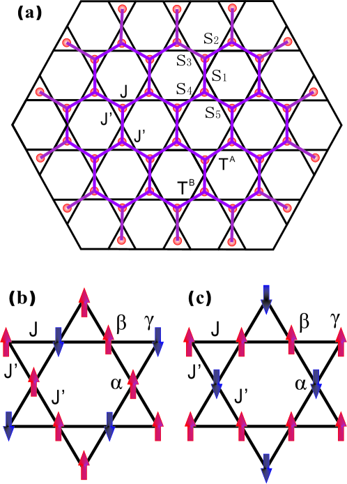
Figure 1: (Color online) (a) The distorted Kagomé lattice, where $J$ and $J^{\prime}$ denote the different nearest neighbor couplings. The dots in the center of small triangles and lines connecting them form a tensor network presented by Eq. (3). (b) and (c) show two degenerate spin configurations of the ferrimagnetic structure, where up and down arrows represent the spin-up and spin-down states, respectively.

In this article, we shall focus on the Ising model on the DK lattice, where the thermodynamics and magnetic properties will be carefully studied by means of exact solutions and a numerical method. In the present model, the quantum fluctuations are completely suppressed, and only the thermal fluctuations are considered. It should be stressed that the present model for $h=0$ can be exactly solved, but for $h\neq 0$ the exact solution is not available at present and the numerical method should be involved in. For this reason, a recently developed tensor renormalization group (TRG) method Levin ; Jiang ; Gu is employed to investigate the thermodynamic properties of the system. The cases with different couplings $J$ and $J^{\prime}$ and both with and without a magnetic field $h$ will be discussed. The TRG results, being consistent with the exact solutions, reveal that the system has ferromagnetic, ferrimagnetic, and paramagnetic phases in the phase diagram, where the paramagnetic phase can exist at $T=0$ in the strongly frustrated region. Moreover, the magnetic order-disorder phase transitions separating these three phases are disclosed. In ferrimagnetic and paramagnetic phases, the $1/3$ magnetization plateaux are seen. A magnetization step at an infinitesimal field is observed for the paramagnetic phase at low temperature. The specific heat no longer possesses a divergent peak once the external field is switched on, implying the absence of phase transitions at $h\neq 0$. In addition, we shall also make an attempt to fit the experimental data of susceptibility for the complex Co(N₃)₂(bpg)$\cdot$ DMF_4/3 with the TRG results so as to estimate the exchange couplings in this complex.

The other parts of this article are organized as follows. In Sec. II, the exact solutions and phase diagrams are presented. The TRG method is introduced in Sec. III. The specific heat without a magnetic field is explored in Sec. IV. Magnetization, susceptibility, and a comparison to the experimental data are shown in Sec. V. Sec. VI contains the results of specific heat in an external magnetic field. The summary and discussions are given finally.

II Exact solutions in zero magnetic field

The Hamiltonian of the system under interest has the form of

$$H=J^{\prime}\sum_{<i\in\alpha,j\in\beta>}{S_{i}S_{j}}+J^{\prime}\sum_{<i\in\alpha,j\in\gamma>}{S_{i}S_{j}}+J\sum_{<i\in\beta,j\in\gamma>}{S_{i}S_{j}}-h\sum_{i}{S_{i}},$$ (1)

where $S_{i}$ is an Ising spin with two discrete values $\pm 1$, and the whole lattice can be divided into three sublattices labeled as $\alpha$, $\beta$, and $\gamma$. The spin-spin coupling terms are restricted to nearest neighbor sites, $J$ and $J^{\prime}$ are different nearest neighboring couplings as shown in Fig. 1, where $J(J^{\prime})>0$ and $<0$ represent antiferromagnetic and ferromagnetic couplings, respectively, $h$ is the uniform external magnetic field, and $g\mu_{B}=1$ is assumed.

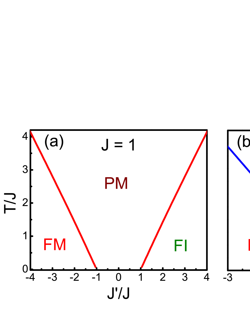
Figure 2: (Color online) The zero-field phase diagrams for different couplings: (a) $J>0$ and (b) $J<0$. The phase boundaries are determined by Eq. (2). In the phase diagrams, FM means ferromagnetic phase, FI represents ferrimagnetic phase, and PM is paramagnetic phase.

Let us first utilize the exact mapping of 2D Ising model onto the 16-vertex model to present the exact solutions on the DK lattice. Following Refs. Diep, ; Diep1, ; Diep2, , for $h=0$, we can write down the free energy per triangle in the thermodynamic limit as

$$f = -\frac{T}{16\pi^{2}}\int_{-\pi}^{\pi}d\theta\int_{-\pi}^{\pi}d\phi\,\ln[a+2b\cos(\theta)$$

$$+ 2c\cos(\phi)+2d\cos(\theta-\phi)+2e\cos(\theta+\phi)],\text{ \ \ \ \ \ \ }(2)$$

where

$$a = \omega_{1}^{2}+\omega_{2}^{2}+\omega_{3}^{2}+\omega_{4}^{2},$$

$$b = \omega_{1}\omega_{3}-\omega_{2}\omega_{4},$$

$$c = \omega_{1}\omega_{4}-\omega_{2}\omega_{3},$$

$$d = \omega_{3}\omega_{4}-\omega_{7}\omega_{8},$$

$$e = \omega_{3}\omega_{4}-\omega_{5}\omega_{6},$$

$$\omega_{1} = 2\exp(-2J/T)[1+\exp(2J/T)\cosh(2J^{\prime}/T)]^{2},$$

$$\omega_{2} = \omega_{1}-8\cosh(2J^{\prime}/T),$$

$$\omega_{3} = \omega_{4}=\omega_{5}=\omega_{6}=\exp(2J/T)\cosh(4J^{\prime}/T)-\exp(2J/T),$$

$$\omega_{7} = \omega_{8}=\omega_{1}-4\exp(-2J/T),$$

where $k_{B}=1$ is presumed. It is straightforward to readily verify that these $\omega$’s satisfy the free-fermion conditions,Diep showing that the Ising model on the DK lattice is exactly solvable. The critical temperature $T_{c}$ at which the phase transition takes place is determined by the following equation

$$1+4\exp(2J/T_{c})\cosh(2J^{\prime}/T_{c})-\cosh(4J^{\prime}/T_{c})=0.$$ (2)

Two different cases are presented in Figs. 2 (a) and (b). When $J>0$, the magnetic ordered phases appear when $|J^{\prime}/J|>1$, which can be recognized as a ferrimagnetic phase for $J^{\prime}/J>1$, and a ferromagnetic phase for $J^{\prime}/J<-1$. This is obtained by checking the magnitude of spontaneous magnetization [see Fig.3 (c) below]. The disordered paramagnetic phase separates the two ordered phases, where the phase boundaries are determined by Eq. (2). For a small $T_{c}$, Eq. (2) can lead to a simple expression $T_{c}/J\approx 2(|J^{\prime}/J|-1)/\ln 4$, that gives the straight phase boundaries in Fig. 2 (a). Notice that the paramagnetic phase exists even at zero temperature owing to the frustration. When $J>0$ and $|J^{\prime}/J|\in[0,1]$, the spin surrounded by $J^{\prime}$ couplings on $\alpha$ sublattice is free to flop up or down without costing energy. Meanwhile, the ground-state spin configurations on $\beta$ and $\gamma$ sublattices are highly degenerate. Hence, the total degeneracy is $K=2^{N/3+N_{c}}$, with $N$ the number of total sites, and $N_{c}$ the number of chains consisting of spins on $\beta$ and $\gamma$ sublattices (the horizontal lines in Fig. 1). This superdegenerate state at zero temperature connects continuously with the paramagnetic phase at finite temperatures. No phase transition appears, and the system is disordered at all temperatures. This observation can also be manifested in Fig. 3 (a), where no singularities exist in the specific heat for $|J^{\prime}/J|=0.4,0.8,1.0$. However, for $|J^{\prime}/J|>1$, as Fig. 2 (a) indicates, there exists a ferromagnetic ($J^{\prime}<0$) or ferrimagnetic ($J^{\prime}>0$) state at low temperatures, and these ordered phases would be destroyed through an order-disorder phase transition with increasing temperature. Correspondingly, the specific heat for $|J^{\prime}/J|=1.2$ in Fig. 3 (a) shows a divergent peak, which is a typical character of second-order phase transition. When $J<0$ [Fig. 2 (b)], the situations are similar, and the system is ordered (ferromagnetic or ferrimagnetic) at low temperatures except for the case $J=-1,J^{\prime}=0$, where the model is degenerated into the decoupled one-dimensional Ising chains, which has $T_{c}=0$ and thus is disordered at any finite temperature.

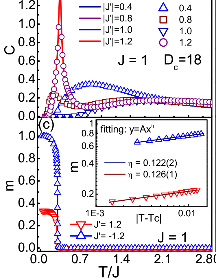
Figure 3: (Color online) Temperature dependence of specific heat and magnetization for different coupling ratio $J^{\prime}/J$ at $h=0$. The TRG results (open symbols) along with the exact solutions (solid and dashed lines) are presented for (a) $J>0$ and (b) $J<0$. In (c) and (d), the magnetization $m$ is plotted for $J>0$ and $J<0$, respectively, where a magnetic order-disorder transition is clearly seen. The insets illustrate the critical behaviors of $m$ near $T_{c}$.

III TRG algorithm

Exact solutions can offer us a reliable phase diagram of the model. However, some other quantities such as the magnetization $m$ and specific heat in nonzero magnetic fields cannot be obtained within the above framework. Hence, we adopt the recently proposed TRG numerical algorithm. The TRG method is first introduced to calculate the 2D classical models,Levin ; Chang and then generalized to study 2D quantum spin models.Jiang ; Li ; Gu ; Chen The principal idea of TRG algorithm is to express the partition function (or the expectation value of quantum operators) as a tensor network, and then utilizes the coarse-graining and decimation procedures to approximately obtain the results. TRG is an efficient method both for classical and quantum spin models.

The first step is to replace each triangle on Kagomé lattice by a tensor, as shown in Fig. 1 (a). The energy of each triangle in an external magnetic field $h$ is $\varepsilon_{\triangle}(s_{1},s_{2},s_{3})=J^{\prime}s_{1}s_{2}+J^{\prime}s_{1}s_{3}+Js_{2}s_{3}-\frac{1}{2}h(s_{1}+s_{2}+s_{3})$. We introduce a three-order tensor $T^{A/B}_{s_{1},s_{2},s_{3}}=\exp(-\varepsilon_{\triangle}(s_{1},s_{2},s_{3})/T)$, where A(B) means down (up)-pointing triangle in Fig. 1 (a). These tensors form a honeycomb lattice, and the partition function can be expressed as

$$Z = \sum_{s_{1},s_{2},s_{3},...=-1,1}\exp\{-[\varepsilon_{\triangle}(s_{1},s_{2},s_{3})+\varepsilon_{\triangle}(s_{1},s_{4},s_{5})+...]/T\}$$ (3)

$$= \sum_{s_{1},s_{2},s_{3},...=-1,1}T^{A}_{s_{1},s_{2},s_{3}}T^{B}_{s_{1},s_{4},s_{5}}...=tTr(T^{A}T^{B}...),$$

where $tTr$ represents the tensor trace. Hence the problem of solving the partition function of Ising model on a DK lattice is equivalently transformed into a honeycomb tensor network problem, which can be efficiently evaluated through the rewiring and coarse-graining iterations (see the details in Ref. Jiang, ). Upon obtaining the partition function $Z$, other thermodynamic quantities can be evaluated straightforwardly. Alternatively, we can also introduce some impurity tensors in the tensor networks to achieve this goal. For example, in order to calculate the magnetization $m$, an impurity tensor $T_{s_{1},s_{2},s_{3}}^{Im}=(\frac{s_{1}+s_{2}+s_{3}}{3})\exp[-1/T\varepsilon_{\triangle}(s_{1},s_{2},s_{3})]$ can be introduced. By replacing one tensor $T^{A/B}$ in Eq. (3), we can get the magnetization per site

$$m=\frac{tTr(T^{Im}T^{B}T^{A}...)}{Z}.$$ (4)

In the following, the second scheme is adopted for evaluating the thermodynamical quantities, such as the magnetization $m$, energy per site $e$, etc.

In our calculations, the number of coarse-graining iterations is generally taken as 20, i.e., the total sites of DK lattice under investigation is $3^{22}\thickapprox 3\times 10^{10}$, which is close to the thermodynamic limit. In addition, the periodic boundary conditions are adopted during the simulations. The initial bond dimension D of tensor $T$ is chosen as 2 owing to the two states (spin-up and -down) of the Ising spins. With the coarse-graining procedure, the bond dimension will increase dramatically, and hence we have to make a truncation and reserve a finite dimension $D_{c}$. In our calculations, $D_{c}$ is taken as high as 18, and the convergence with various $D_{c}$ has always been checked.

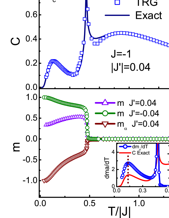
Figure 4: (Color online) The specific heat and magnetization $m$ as functions of temperature with $|J^{\prime}/J|=0.04$ at $h=0$. (a) Specific heat, where three peaks appear, one of which is divergent; (b) Magnetization $m$ and sublattice magnetization $m_{\alpha}$, where $|m_{\alpha}|$ decreases rapidly (but does not vanish) around the peak position of the specific heat at low temperature, which is also revealed as a local maximum of $dm_{\alpha}/dT$ in the inset.

IV Specific Heat and Phase Transitions

When $h=0$, both exact solution and TRG method can be utilized to evaluate the specific heat. In Figs. 3 (a) and (b), the TRG results are plotted by symbols, while the exact results by lines. Excellent agreement can be observed, except for the region around the critical point where a divergent peak occurs. Another character is that the specific heat at zero field is independent of the sign of coupling $J^{\prime}$, but is relevant to the magnitude of $|J^{\prime}|$. In Fig. 3 (a), when $|J^{\prime}|$ is small, there is only one round peak in the specific heat. By tuning $|J^{\prime}|$ to approach $J$ from below (e.g. $|J^{\prime}|/J=0.8$), a new round peak appears at low temperature, which disappears when $|J^{\prime}|=J$ and the system again exhibits a single round peak. These observations imply that there exist no phase transitions when $|J^{\prime}|\leq J$, which is owing to the strong frustration, and is in accordance with the phase diagram in Fig. 2 (a). Furthermore, if $|J^{\prime}|$ exceeds $J$ [as $|J^{\prime}/J|=1.2$ in the Fig. 3 (a)], a divergent peak emerges, implying the occurrence of phase transition. In Fig. 3 (b), a typical curve of specific heat with $|J^{\prime}/J|=1$ is shown. A divergent peak occurs at the transition temperature $T_{c}\approx 2.14$, again in agreement with the exact solution ($T_{c}=4/\ln(3+2\sqrt{3})$). Moreover, the specific heat is logarithmically divergent at the critical point because of $2\exp(2J/T_{c})+\cosh(4J^{\prime}/T_{c})-1\neq 0$, as shown in Figs. 3 (a) and (b).

The phase transitions can also be verified by studying the order parameter, i.e., the magnetization per site $m$ defined in Eq. (4). In Figs. 3 (c) and (d), when $J=1,J^{\prime}/J>1$ or $J=-1,J^{\prime}>0$, $m=1/3$ at $T=0$ and remains finite at small temperatures. This nonzero spontaneous magnetization implies the existence of a ferrimagnetic phase; while $J=1,J^{\prime}/J<-1$ or $J=-1,J^{\prime}<0$, the magnetization starts from $m=1$, and the system is in a ferromagnetic phase when $T$ is smaller than the critical temperature $T_{c}$. With increasing temperature, $m$ decreases steeply to zero in the vicinity of $T_{c}$, showing a order-disorder phase transition happens. In addition, the critical behavior of $m$ near $T_{c}$ has been investigated. In the insets of Figs. 3 (c) and (d), in terms of $m\propto(T_{c}-T)^{\eta}$, the fittings in different cases coincidentally give $\eta\simeq 1/8$, which is the same as that of Ising model on a square lattice.Yang The phase transition occurring at $T_{c}$ probably falls into the universality class of 2D Ising models.

Another interesting case is shown in Fig. 4 (a), where the temperature dependence of the specific heat is presented for $J<0$ and $|J^{\prime}|\ll|J|$. One may note that there are three peaks, including two round peaks and a divergent one. Both exact solutions and TRG method give the same results. In order to investigate the origin of each peak, the TRG method is utilized to calculate the magnetization $m$ and sublattice magnetization $m_{\alpha}$. As shown in Fig. 4 (b), $m$ behaves rather differently for $J^{\prime}=0.04$ and $-0.04$, although the specific heat coincides for both. When $J^{\prime}=-0.04$, the ground state is ferromagnetic, and $m$ decreases monotonously with increasing temperature and vanishes sharply at critical temperature $T_{c}$. The case with $J^{\prime}=0.04$ is more interesting, where the system possesses a ferrimagnetic ground state with $m=1/3$ at $T=0$. With increasing temperature, $m$ first increases until the temperature is close to the critical point $T_{c}$, and then goes down steeply to zero. In order to understand this peculiar behavior, we have plotted the sublattice magnetization $m_{\alpha}$ as a function of $T$ in Fig. 4 (b). In the ferrimagnetic case, $m_{\alpha}$ is aligned anti-parallel with the spins on the other two sublattices, and its magnitude decreases rapidly with increasing temperature owing to the coupling $J^{\prime}$ weak. Hence, $m=(-|m_{\alpha}|+m_{\beta}+m_{\gamma})/3$ would first increase until the temperature approaches to $T_{c}$, where $m_{\alpha}$, $m_{\beta}$, and $m_{\gamma}$ disappear simultaneously. Moreover, as the inset shows, the first-order derivative $dm_{\alpha}/dT$ has a round peak at the temperature $T_{r}$, which coincides with the low temperature peak position of specific heat. Although $m_{\alpha}$ decreases rapidly around $T_{r}$, it does not vanish. It should be pointed out that $T_{r}$ is not a critical point, as the specific heat shows only a round peak and never diverges at $T_{r}$.

V Magnetization and Susceptibility

V.1 Magnetization Plateaux and Ground State Phase Diagrams

When the external magnetic field is switched on, the exact solution in Sec. II no longer works. The TRG method, which has been verified to be accurate and reliable in the previous sections, is utilized to study the response of the system to an external magnetic field.

Figure 5: (Color online) In (a) and (b), the magnetic curves for different couplings for $J>0$ and $J<0$ are shown, respectively, where $|T/J|=0.2$ and $D_{c}$=18. Inset in (b) presents the magnetic curves with different temperatures below and above $T_{c}$. In (c) and (d), the ground-state phase diagrams on $J^{\prime}-h$ plane are presented.

Let us first focus on the magnetization, where the $1/3$ magnetization plateaux are obtained, as shown in Fig. 5. When $J>0$ and $J^{\prime}/J\in[-1,1]$ in Fig. 5 (a), the system is in a paramagnetic phase at all temperatures. An infinitesimal small magnetic field can polarize the free spin on $\alpha$ sublattice at $T=0$, and hence drives the ground state to a ferrimagnetic state with $m=1/3$ after a magnetization jump, and the $1/3$ plateaux appear in the magnetization curves. At finite but small temperatures, these plateaux are still present. This field-induced $1/3$ plateau ferrimagnetic phase is highly degenerate, and the degeneracy is $K=2^{N_{c}}$, where $N_{c}$ is the number of independent spin chains in the system. One of the degenerate spin configurations is shown in Fig.1 (b). When the field is larger than a critical field $h_{c}$, the spins on $\beta$ and $\gamma$ sublattices align parallel instead of antiparallel, and the system has the saturated magnetization $m=1$, leading to a ferromagnetic spin configuration. The energy difference per site between the polarized ferromagnetic and the plateau ferrimagnetic state is $\delta e=\frac{4}{3}(J^{\prime}+J)$. The Zeeman energy $\delta e_{z}=-\frac{2}{3}h$ at the critical magnetic field $h_{c}$ has to compensate this energy difference. $\delta e_{z}+\delta e=0$ leads to $h_{c}=2(J+J^{\prime})$, as verified in Fig. 5 (a), where the critical field $h_{c}$ increases with enhancing the coupling $J^{\prime}$. In addition, there exists a notable difference between the magnetization curves of $J^{\prime}=1.2$ and others in Fig. 5 (a). The former starts from a nonzero spontaneous magnetization ($m=1/3$) owing to its ferrimagnetic ground state instead of a paramagnetic one. The ground state spin configuration for $J^{\prime}>1$ is illustrated in Fig. 1 (c), which is ferrimagnetically ordered. Considering the spontaneously broken $Z_{2}$ symmetry, this ground state is no longer degenerate. Hence, the width of $1/3$ plateau does not obey the relation mentioned above, but has another relation in the ferrimagnetic case to be discussed below.

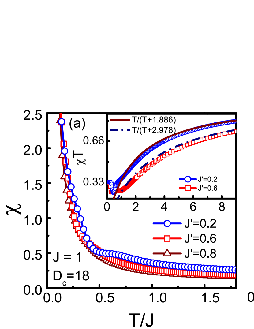
Figure 6: (Color online) Temperature dependence of zero-field susceptibility for different $J$ and $J^{\prime}$. (a) $\chi$ diverges at $T=0$ and $\chi T$ converges to 1/3 as the inset shows; (b) $\chi$ shows divergent peaks at the critical temperature $T_{c}$, where the magnitude of $\chi$ with $J=J^{\prime}=-1$ has been divided by two. The susceptibility is calculated at $h=0.01$ and, the convergence with various small fields has been checked.

For $J<0$, there exist ferromagnetic ($J^{\prime}<0$) and ferrimagnetic ($J^{\prime}>0$) ground states. The cases with $J^{\prime}>0$ possess $m=1/3$ plateaux, as seen in Fig. 5 (b). Comparing with the former case $J>0$, the width of $1/3$ plateaux has a different relation with couplings $J$ and $J^{\prime}$. By identifying $\delta e=\frac{8}{3}J^{\prime}$ and $\delta e_{z}=-\frac{2}{3}h$, $h_{c}=4J^{\prime}$ is obtained, that is independent of $J$. Here, the spin configuration on $m=1/3$ plateau is illustrated in Fig. 1 (c). The order parameter characterizing this phase is the spontaneous magnetization $m|_{h=0}$, which implies the breaking of $Z_{2}$ symmetry. By increasing temperature, the $Z_{2}$ symmetry will eventually recover above the critical temperature $T_{c}$, and the spontaneous magnetization will vanish. As shown in the inset of Fig. 5 (b), the magnetization at $T>T_{c}$ starts from $m=0$, and the $1/3$ plateau is smeared and finally destroyed by strong thermal fluctuations.

In order to look at the effects of external magnetic fields, the phase diagrams at zero temperature are plotted in Figs. 5(c) and (d). For $J>0$, as shown in Fig. 5 (c), there are four different phases including ferromagnetic, ferrimagnetic, plateau ferrimagnetic, and disorder phase that only exists in the $h=0$ line. It is worthwhile emphasizing that although the magnetization in the $1/3$ plateau ferrimagnetic phase has the same value as that in the ferrimagnetic phase at $T=0$, they are quite different in nature. The former is induced by a magnetic field and highly degenerate with the degeneracy $K=2^{N_{c}}$, while the latter is an spontaneously ordered phase with the $Z_{2}$ symmetry breaking. As indicated in Fig. 5 (d), for $J<0$, only a ferrimagnetic phase and a ferromagnetic phase exist. Here we would like to stress that the phase transitions between these different phases only occur at $T=0$, and the temperature would then blur the transitions. In fact, in the presence of an external magnetic field, there are no thermodynamic phase transitions at finite temperatures, which will be discussed in Sec. VI.

V.2 Susceptibility

In order to understand the magnetic response of the present system to an external magnetic field, the zero-field susceptibility $\chi$ is obtained by $\chi=[m(h)-m(h=0)]/h$ for a small magnetic field. In Fig. 6 (a), where $J=1$ and $J^{\prime}\in(0,1)$, the ground state is disordered, and the spins on one ($\alpha$) sublattice are free to flip up or down without an energy cost due to the frustration effect. $\chi$ diverges, obeying Curie law, i.e., $\chi\propto 1/T$ as $T$ approaches zero. This result is validated in the inset of Fig. 6 (a), where the $\chi T$ curves converge to a constant $1/3$ at low temperatures, which is independent of $J^{\prime}$. The specific value $1/3$ can be attributed to the free spins on one of three sublattices. On the other hand, in the high temperature limit, $\chi$ decays with the Curie-Weiss law, which can be fitted by $\chi T=\frac{T}{T+\theta}$ up to $T/J=100$ (Note that Fig. 6 shows only to $T/J\simeq 9$). It is straightforward to use the mean-field approximation to obtain the Curie-Weiss temperature $\theta$ as $(8J^{\prime}+4J)/3$, and $\theta=1.867$ and $2.933$ for $J^{\prime}=0.2$ and $0.6$, respectively. The fittings in the inset of Fig. 6 (a) agree with the mean-field predictions, that further validates our TRG results. In Fig. 6 (a), it is interesting to notice that there exists a turning point at an intermediate temperature in the crossover region, which separates the low $T$ Curie behavior and high $T$ Curie-Weiss behavior, as shown in the inset of Fig. 6(a). Quite differently, as seen in Fig. 6 (b), when the ground state is ferrimagnetically or ferromagnetically ordered, the susceptibility has a divergent peak at $T_{c}$ where the magnetic ordering is destroyed by thermal fluctuations. This again certifies the existence of magnetic order-disorder phase transitions.

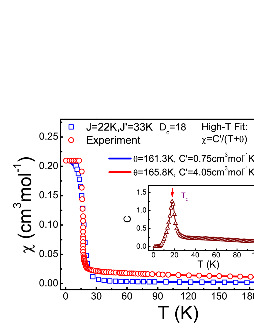
Figure 7: (Color online) A comparison of TRG results to the experiment, where the experimental data are taken from Ref. Gao, . The TRG result is calculated at a small field $h/J=0.05$. The high temperature fittings with the Curie-Weiss law to both experimental and TRG results are also shown. The inset predicts a divergent peak in the specific heat around $T=20$K.

V.3 Comparison to Experiments

The complex Co(N₃)₂(bpg)$\cdot$ DMF_4/3 reported in Ref. Gao, is a molecular magnetic material, in which the Co⁺² ions form a distorted Kagomé layer. Experimentally, the susceptibility does not go to zero as $T$ approaches zero (see Fig. 7), which is unusual for an isotropic Heisenberg antiferromagnetic system. In fact, the Co⁺² ions are believed to have effective spin-1/2 when $T\leq$ 20K, with anisotropic Lande $g$ factors ( $g_{\parallel}\neq 0$, $g_{\perp}\approx 0$), which implies that in this compound the Ising-type couplings may be dominant between Co⁺² ions.Carlin ; xyWang Here, we try to use our TRG results to fit the experimental data of susceptibility (especially for the low $T$ region) for this complex. To be consistent with the experimental convention, the definition of susceptibility $\chi=m(h)/h$ is adopted. As shown in Fig. 7, $\chi$ decreases steeply around the transition temperature and, one may see that the fittings agree rather well with the experimental data at low temperatures. The exchange coupling constants for this compound are estimated through the fittings as $J=22K$ and $J^{\prime}=33K$. According to our study on the Ising DK lattice with the parameters $J>0$ and $J^{\prime}/J=1.5$, the system has a ferrimagnetic phase at low temperatures. It is thus not difficult to understand why the low temperature susceptibility goes to a finite value instead of zero for this compound. At high temperatures, by fitting the TRG results with the Curie-Weiss law $\chi=C^{\prime}/(T+\theta)$, we find that the Curie-Weiss temperature $\theta\thickapprox 161.3K$, which agrees well with that of experimental estimation ($\theta\thickapprox 165.8K$, see online supporting material of Ref. Gao, ). Besides, we find that the ratio of the experimental susceptibility to the result from the Ising model equals a constant $R\approx 5.4$ in the high temperature limit. This constant ratio may be ascribed to the fact that in the material at $T>$20K the effective spin of Co⁺² ions may no longer be 1/2 and also, the other interactions such as XY couplings may intervene, giving rise to that the Ising model is insufficient to describe the behaviors of this complex. Surely, more experimental results towards this direction are needed. In addition, we have calculated the specific heat based on the Ising model with the couplings given above, and found that a divergent peak exists around $T=20$K, as depicted in the inset of Fig. 7, suggesting that this compound may undergo a phase transition at low temperature. Experimental studies on the specific heat and other quantities for this compound will be carried out in near future.

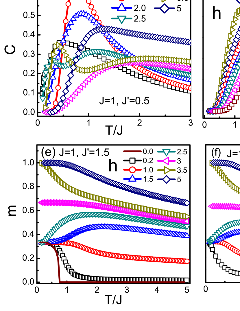
Figure 8: (Color online) The specific heat $C$ and the magnetization $m$ as functions of temperature in different magnetic fields. (a), (b) and (e) illustrate the ferrimagnetic case $J>0,J^{\prime}/J=1.5$, (c) and (f) are for the paramagnetic case $J>0,J^{\prime}/J=0.5$, and (d) depicts the ferromagnetic case $J>0,J^{\prime}/J=-1.5$.

VI Specific Heat and magnetization in a Magnetic Field

Next, we will study the effect of an external magnetic field on the specific heat. Three typical cases will be studied: ferrimagnetic ($J>0,J^{\prime}/J=1.5$), paramagnetic ($J>0,J^{\prime}/J=-0.5$), and ferromagnetic ($J>0,J^{\prime}/J=-1.5$) cases.

In Fig. 8, the specific heat in the presence of an external field for the ferrimagnetic case ($J>0$, $J^{\prime}/J>1$) is shown. Fig. 8(a) shows at small fields with $h\leq 2J$, the peak of specific heat moves towards high temperatures, and its height firstly decreases, and then increases with enhancing the field until it approaches the spin flop critical field $h_{c}$, which polarizes all spins. In Fig. 8(b), when the field keeps increasing, the peak of specific heat becomes dulled, and then splits into double peaks (except for the point $h=h_{c}$), which can be viewed as a field-induced splitting. Similar phenomena have also been observed in other Ising and Heisenberg spin systems.Gong ; Li2 The double peak scenario will eventually be spoiled by further increasing $h$. When $h\gg h_{c}$, the specific heat will again be single-peaked. It is notable that the divergent peaks at zero field disappear immediately when the field is switched on, which means that the phase transitions are absent and the system remains in the ferrimagnetic phase at all temperatures. When $h=0$, the ferrimagnetic ordered phase spontaneously breaks the $Z_{2}$ symmetry contained in the Hamiltonian (see Eq. 1), and possesses a nonzero order parameter. When $T>T_{c}$, the thermal fluctuations will destroy the magnetic order, while $Z_{2}$ symmetry will be recovered, and $m$ vanishes immediately [the solid line in Fig. 8 (e)]. However, the external field explicitly breaks the $Z_{2}$ symmetry in the Hamiltonian, and $m$ is nonzero even at high temperature $T>T_{c}$ [the symbol lines in Fig. 8 (e)]. Therefore, no phase transition occurs in the presence of a magnetic field. In Fig. 8(e), according to the magnetization $m$ at zero temperature, the curves can be classified into three classes. When $h<h_{c}$, the curves start from $m=1/3$; while $h>h_{c}$, the spins are polarized and $m=1$ at $T=0$; when $h=h_{c}$, the case is of a little subtlety, where $m$ equals to the statistical mean value $2/3$ at zero temperature.

In Figs. 8 (c) and (f), the paramagnetic case $J>0,J^{\prime}/J=0.5$ is studied. The field will firstly promote the peak height of the specific heat, and moves the peak to the high temperature side. When $h$ is close to the critical field, the specific heat will again be dulled, where the height is decreasing, and the peak splits into two sub peaks except at the point $h=h_{c}$. When the field $h\gg h_{c}$ a single peak of the specific heat recurs. The $m-T$ curves in Fig. 8 (f) are quite similar to those in Fig. 8 (e) and can be classified analogously. At last, the ferromagnetic case $J>0,J^{\prime}/J<-1$ is shown in Fig. 8 (d). The divergent peak for the ferromagnetic-paramagnetic phase transition disappears owing to the same reason in the ferrimagnetic case as mentioned above. The specific heat reveals a round peak, which moves towards the high temperature side. By continuously enhancing the field, the height of the peak decreases down firstly and then goes slowly up.

Besides, we have also studied other situations with different couplings, and found that they can be ascribed into the above three classes. For instance, other ferrimagnetic cases with $J<0,J^{\prime}>0$ and ferromagnetic cases with all ferromagnetic couplings ($J,J^{\prime}<0$) behave similarly with those presented in Fig. 8.

VII Summary and discussion

In this article, we have systematically studied the thermodynamics and magnetic properties of Ising model on a DK lattice by exact solutions and the TRG numerical method. It is shown that the phase diagrams are composed of three phases including ferromagnetic, ferrimagnetic, and paramagnetic phases. Phase transitions between them are identified by studying the specific heat and magnetization. The critical exponent $\eta$ of $m$ near $T_{c}$ is determined as $1/8$, which appears to fall into the universality of the 2D Ising models. The TRG results of zero-field specific heat agree very well with the exact solutions, showing that TRG is an efficient and accurate tool in dealing with 2D Ising models. The TRG method is also utilized to study the properties in the presence of a magnetic field. In the magnetization curves, $1/3$ plateaux at low $T$ are identified and, the relations of the plateau width with coupling constants $J,J^{\prime}$ are obtained. In addition, the zero temperature $J^{\prime}-h$ phase diagrams are presented to clarify the various ground state phases in external magnetic field. The zero-field susceptibility $\chi$ of the paramagnetic case ($J>0,|J^{\prime}/J|\leq 1$) is found to obey Curie law at low $T$ and Curie-Weiss law at high $T$. While in the ferrimagnetic or ferromagnetic case, the divergent peak of $\chi$ is found at the critical temperature. Moreover, the specific heat under different magnetic fields is also investigated. It is uncovered that the phase transitions are absent immediately when a magnetic field is switched on, and the field-induced peak splitting of the specific heat is recognized when $h$ is close to the critical field. We have also fitted the experimental data of susceptibility of the complex Co(N₃)₂(bpg)$\cdot$ DMF_4/3 with the TRG results, and obtained the couplings $J=22$K and $J^{\prime}=33$K. Based on TRG calculations, a ferrimagnetic-paramagnetic phase transition is expected to occur at about $T=20$K in this complex, which will be studied in future. The present study offers a systematic understanding for physical properties of the 2D Ising model on the DK lattice, and will be useful for analyzing future experimental observations in related magnetic materials with DK lattices.

- (1) P. Lecheminant, B. Bernu, C. Lhuillier, L. Pierre, and P. Sindzingre, Phys. Rev. B 56, 2521 (1997).
- (2) H. C. Jiang, Z. Y. Weng, and D. N. Sheng, Phys. Rev. Lett. 101, 117203 (2008).
- (3) See, for instance, U. Schollwök, J. Richter, and D. J. J. Farnell, and R. F. Bishop, Quantum Magnetism, Lect. Notes Phys. 645 (Springer, Berlin, 2004), Chapter 2, and references therein.
- (4) Fa Wang, Ashvin Vishwanath, and Yong Baek Kim, Phys. Rev. B 76, 094421 (2007).
- (5) Andreas P. Schnyder, Oleg A. Starykh, and Leon Balents, Phys. Rev. B 78, 174420 (2008).
- (6) M. Yoshida, M. Takigawa, H. Yoshida, Y. Okamoto, and Z. Hiroi, Phys. Rev. Lett. 103, 077207(2009).
- (7) H. Yoshida, Y. Okamoto, T. Tayama, et.al., J. Phys. Soc. Jpn. 78, 043704 (2009).
- (8) J. N. Behera and C. N. R. Rao, Inorg. Chem. 45, 9475 (2006).
- (9) Xin-Yi Wang, Lu Wang, Zhe-Ming Wang, and Song Gao, J. Am. Chem. Soc. 128, 674 (2006).
- (10) R. Kaneko, T. Misawa, and M. Imada, arXiv:1004.2401v1 (2010).
- (11) K. Hida, J. Phys. Soc. Jpn. 70, 3673 (2001).
- (12) Richard L. Carlin, Magnetochemistry, (Springer-Verlag, Berlin, 1986), P29-30, P65-69, and references therein.
- (13) M. Levin and C. P. Nave, Phys. Rev. Lett. 99, 120601 (2007).
- (14) H.C. Jiang, Z.Y. Weng, and T. Xiang, Phys. Rev. Lett. 101 090603 (2008); Z.Y. Xie, H.C. Jiang, Q.N. Chen, Z.Y.Weng, and T. Xiang, Phys. Rev. Lett. 103, 160601 (2009); H. H. Zhao, Z. Y. Xie, Q. N. Chen, Z. C. Wei, J. W. Cai, and T. Xiang, Phys. Rev. B 81, 174411 (2010).
- (15) Z. C. Gu, M. Levin, and X. G. Wen, Phys. Rev. B 78, 205116 (2008).
- (16) H. T. Diep and H. Giacomini, Frustrate Spin Systems, ed. H. T. Diep (World Scientific, Singapore, 2005) p. 1.
- (17) P. Azaria, H. T. Diep, and H. Giacomini, Phys. Rev. Lett. 59, 1629 (1987).
- (18) M. Debauche, H. T. Diep, P. Azaria, and H. Giacomini, Phys. Rev. B 44, 2369 (1991).
- (19) Ming-Che Chang, Min-Fong Yang, Phys. Rev. B 79, 104411 (2009).
- (20) Wei Li, Shou-Shu Gong, Yang Zhao, and Gang Su, Phys. Rev. B 81, 184427 (2010).
- (21) P. Chen, C.Y. Lai, and M.F. Yang, J. Stat. Mech. P10001 (2009).
- (22) C. N. Yang, Phys. Rev. 85, 808 (1952).
- (23) We thank X. Y. Wang for discussions about the low temperature magnetic properties of Co+2 ions.
- (24) Shou-Shu Gong, Song Gao, and Gang Su, Phys. Rev. B 80, 014413 (2009).
- (25) Wei Li, Shou-Shu Gong, Yang Zhao, Ziyu Chen, and Gang Su, Phys. Lett. A 374, 2589 (2010).