Soft spectator scattering in the nucleon form factors at large $Q^{2}$ within the SCET approach

Abstract

The proton form factors at large momentum transfer are dominated by two contributions which are associated with the hard and soft rescattering respectively. Motivated by a very active experimental form factor program at intermediate values of momentum transfers, $Q^{2}\sim 5-15~{}\text{GeV}^{2}$, where an understanding in terms of only a hard rescattering mechanism cannot yet be expected, we investigate in this work the soft rescattering contribution using soft collinear effective theory (SCET). Within such a description, the form factor is characterized, besides the hard scale $Q^{2}$, by a hard-collinear scale $Q\Lambda$, which arises due to the presence of soft spectators, with virtuality $\Lambda^{2}$ ($\Lambda\sim 0.5$ GeV), such that $Q^{2}\gg Q\Lambda\gg\Lambda^{2}$. We show that in this case a two-step factorization can be successfully carried out using the SCET approach. In a first step (SCET_I), we perform the leading-order matching of the QCD electromagnetic current onto the relevant SCET_I operators and perform a resummation of large logarithms using renormalization group equations. We then discuss the further matching onto a SCET_II framework, and propose the factorization formula (accurate to leading logarithmic approximation) for the Dirac form factor, accounting for both hard and soft contributions. We also present a qualitative discussion of the phenomenological consequences of this new framework.

I Introduction

The study of the nucleon form factors (FFs) is one of the central topics in hadronic physics ( for recent reviews see, e.g. , Refs. HydeWright:2004gh ; Arrington:2006zm ; Perdrisat:2006hj ). Substantial progress has been achieved in this field over the past decade, mainly thanks to new experimental methods, using polarization observables, which allow for precise measurements of the FFs. The results for the proton FFs, obtained over the past few years at JLab Jones00 ; Punjabi:2005wq ; Gayou02 ; Puckett:2010ac up to a momentum transfer $Q^{2}\simeq 8.5$ GeV², considerably boosted our knowledge about the distribution of the electric charge inside the proton. A substantial program to extend the measurements of the nucleon FFs up to $Q^{2}\simeq 15$ GeV² in the spacelike region will be performed in the near future at the JLab $12$ GeV upgrade. In parallel, the PANDA Collaboration at GSI is planning to carry out precise measurements of the proton FFs at large timelike momentum transfers, up to around 20 GeV², using the annihilation process $p+\bar{p}\rightarrow e^{+}+e^{-}$ Sudol:2009vc . These experiments will provide us with precious information on the FF behaviors in the region of large momentum transfers.

On the theory side, an understanding of the nucleon FFs at large momentum transfers, both spacelike and timelike, from the underlying QCD dynamics, still remains a challenge. At present, the FF behavior for moderate and large values of $Q^{2}$ is still not well understood and an adequate description, allowing for quantitative predictions, is absent.

The leading power behavior of the FFs was studied a long time ago using the QCD factorization approach ( see, e.g., Chernyak:1983ej ; Lepage:1979zb and references therein). It was established that the dominant contribution can be represented by a reduced diagram as shown in Fig.1.

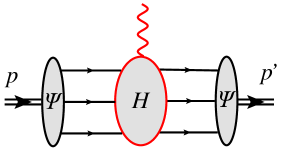
Figure 1: Reduced diagram describing the hard scattering picture

In this figure, the hard blob describes the hard scattering of quarks and gluons with virtualities of order $Q^{2}$. Such a hard subprocess can be systematically computed in perturbative QCD (pQCD) order-by-order. The soft blobs, denoted by $\mathbf{\ \Psi}$, describe the soft, nonperturbative subprocesses, and can be parametrized in terms of universal matrix elements known as distribution amplitudes (DAs). Such a picture suggests the well known factorization formula for the Dirac FF

$$F_{1}=\int dx_{i}~{}\int dy_{i}~{}\mathbf{\Psi}(x_{i})~{}\mathbf{H}(x_{i},y_{i}|Q)~{}\mathbf{\ \Psi}(y_{i})\equiv\mathbf{\Psi}*\mathbf{H}*\mathbf{\Psi},$$ (1)

and predicts the scaling behavior

$$F_{1}\sim\frac{\Lambda^{4}}{Q^{4}}\times\left[\ln Q/\Lambda\right]^{\gamma},$$ (2)

where the logarithmical corrections can be systematically computed order-by-order.

Unfortunately, for the Pauli FF $F_{2}$ this approach cannot provide such a systematic picture and suggests only the power estimate

$$F_{2}\sim\frac{\Lambda^{6}}{Q^{6}}.$$ (3)

Almost simultaneously, it was found that the picture described by Fig.1 is not complete. In Ref. Dun1980 it was demonstrated that the exchange of soft quarks between initial and final states may also produce contribution of order $1/Q^{4}$ times logarithms. In Refs. Fadin1981 ; Fadin1982 all such contributions were computed with the leading logarithmic accuracy at 2 and 3 loops. Using these results it was assumed Fadin1982 that these “nonrenormalization” logarithms probably can be resummed to all orders into an exponent similar to the well known Sudakov logarithms Sudakov:1954sw . However, this effect was ignored in many later publications. In particular, in Ref. Lepage:1979zb it was suggested that such contributions could be strongly suppressed due to those Sudakov logarithms and therefore can be ignored at large values of $Q^{2}$.

At the same time, many phenomenological studies of the hard rescattering picture support the conclusion that in the region of moderate $Q^{2}\simeq 5-10~{}$GeV² the factorization approach expressed by Eq. (1) cannot describe the data properly ( see, for instance, Bolz:1994hb ). Moreover, existing data for the FF ratio $F_{2}/F_{1}$ measured up to $Q^{2}=8.5~{}$GeV² Puckett:2010ac also do not support the expectation of Eq. (3) which assumes that in the asymptotic region $Q^{2}F_{2}/F_{1}\sim const.$ Therefore, it was suggested that the so-called Feynman mechanism Feynman:1973xc , associated with the scattering of the hard virtual photon off one active quark, dominates the nucleon FFs at moderate values of $Q^{2}$. The other spectators remain soft and therefore very often such scattering is associated with the soft overlap of the nucleon wave functions.

Such a picture is supported by different phenomenological approaches, such as QCD-motivated models for the hadronic wave functions Isgur:1984jm ; Isgur:1988iw ; Isgur:1989cy , QCD sum rules Ioffe:1982qb ; Nesterenko:1982gc and light-cone sum rules Braun:2001tj ; Braun:2006hz . The Sudakov suppression in this case is always assumed to be relatively small. The aim of the present work is to develop a systematic approach for the specific soft contribution described first in Ref. Dun1980 , and formulate it through a factorization theorem. We apply the effective theory approach, known as soft collinear effective theory (SCET), in order to describe contributions from different regions of virtualities in the diagrams.

The effective theory is a very convenient tool in this case because soft rescattering is characterized by subprocesses which exhibit different scales : a hard rescattering involving particles with momenta of order $Q^{2}$, hard-collinear scattering processes with virtualities of order $\Lambda Q$, and soft nonperturbative modes with momenta of order $\Lambda^{2}$. Therefore one has to perform a two-step matching procedure in order to perform full factorization of such a process.

Following this scheme we obtain that the full description of large-$Q^{2}$ behavior of the nucleon FF $F_{1}$ is given by the sum of two contributions associated with the soft and hard rescattering picture:

$$F_{1}\simeq F_{1}^{(s)}+F_{1}^{(h)}.$$ (4)

The hard rescattering part $F_{1}^{(h)}$ is well known and described by (1). One can expect that the soft contribution can also be presented in a factorized form but with the more complicated structure reflecting the presence of different scales. Performing the leading logarithmic analysis of the leading power contribution ($\sim 1/Q^{4}$) we demonstrate in this work that the corresponding soft term can be presented in the following form,

$$F_{1}^{(s)}\simeq H(Q)\int Dy_{i}\mathbf{\Psi}(y_{i})\int_{0}^{\infty}d\omega_{1}d\omega_{2}~{}\mathbf{J}^{\prime}(y_{i},\omega_{i}Q)\int Dx_{i}\mathbf{\Psi}(x_{i})\int_{0}^{\infty}d\nu_{1}d\nu_{2}~{}\mathbf{J}(x_{i},\nu_{i}Q)\boldsymbol{S}(\omega_{i},\nu_{i}),$$ (5)

which can be interpreted in terms of a reduced diagram as in Fig.2. This result involves a hard coefficient function $H$, and two hard-collinear jet functions $\mathbf{J}$ and $\mathbf{J}^{\prime}$ which can be computed in pQCD. They describe the subprocesses with hard momenta and hard collinear momenta respectively. The nonperturbative functions $\mathbf{\Psi}$ and $\boldsymbol{S}$ describe the scattering of collinear and soft modes. The convolution integrals in Eq. (5) are performed with respect to the collinear fractions $x_{i}$ and $y_{i}$, and with respect to the soft spectator fractions $\omega_{i},\nu_{i}\sim\Lambda$.

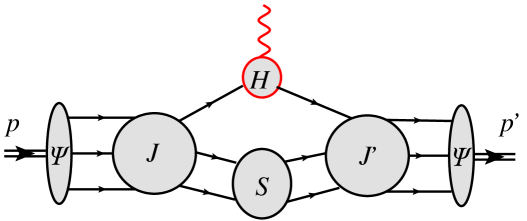
Figure 2: Interpretation of the soft rescattering as a reduced diagram

In the case of the Pauli FF $F_{2}$, we can also perform a factorization of the soft-overlap contribution but only partially, separating the hard modes with momenta of order $Q^{2}$. The full factorization is problematic due to overlapping integration regions corresponding with soft and collinear contributions, which lead to well known end-point singularities in the convolution integrals. However, such a partial result can be used to carry out a phenomenological analysis of the FFs in the region of intermediate $Q^{2}$ values. Such a region corresponds to momentum transfers where $Q^{2}$ is large enough, allowing us to perform a power expansion, but where the second, hard-collinear scale $\sim\Lambda Q$ is still relatively small, so that one expects the dominance of the leading power asymptotic term. Such a situation may indeed be relevant to interpret existing data and planned experiments.

The specific feature of the factorization for the soft-overlap contribution is the presence of the Sudakov logarithms which can be ressummed using the renormalization group in effective field theory. It was suggested, see e.g. Radyushkin00 , that these logarithms could play an important role in the timelike region providing an enhancement of the timelike FFs compared to the spacelike region (the so-called $K$ factor). Within the factorization picture such an enhancement can be clearly studied in a model independent way.

Our paper is organized as follows. In Sec. II , we consider as an example the analysis of the dominant regions for certain Feynman diagrams and demonstrate the existence of the soft spectator contribution at leading power (in the hard scale $Q$) for both the Dirac and Pauli FFs. In Sec. III, we discuss the factorization scheme for such contributions, perform the leading-order matching between QCD and the SCET, and perform a resummation of large logarithms. In Sec. IV we discuss the SCET power counting in $1/Q$ and derive the factorization formula (5). In Sec. V, we perform a first qualitative discussion of the phenomenological consequences following from our results. In Sec. VI, we summarize our findings.

II Soft rescattering mechanism: examples

In this section we consider specific examples of soft rescattering contributions. For the Dirac FF our analysis overlaps with results of the work of Ref. Dun1980 , whereas for the Pauli FF this is discussed here for the first time.

In our consideration we use the Breit frame

$$q=p^{\prime}-p=Q\left(\frac{n}{2}-\frac{\bar{n}}{2}\right),~{}\ n=(1,0,0,-1),~{}\bar{n}=(1,0,0,1),~{}\ (n\bar{n})=2,~{}$$ (6)

and define the external momenta as

$$p=\mathcal{Q}\frac{\bar{n}}{2}+\frac{m_{N}^{2}}{\mathcal{Q}}\frac{n}{2},~{}\ \ p^{\prime}=\mathcal{Q}\frac{n}{2}+\frac{m_{N}^{2}}{\mathcal{Q}}\frac{\bar{n}}{2},~{}\ \ \mathcal{Q=}Q\frac{1}{2}\left[1+\sqrt{1+\frac{4m_{N}^{2}}{Q^{2}}}\right]=Q+\mathcal{O}(m_{N}^{2}/Q^{2}),$$ (7)

$$~{}\ 2(pp^{\prime})=\mathcal{Q}^{2}+\frac{m_{N}^{4}}{\mathcal{Q}^{2}}\approx Q^{2},$$ (8)

where $m_{N}$ is the nucleon mass. For the incoming and outgoing collinear quarks we always imply

$$p_{i}=x_{i}\mathcal{Q}\frac{\bar{n}}{2}+p_{\bot i}+\left(x_{i}^{\prime}~{}\frac{m_{N}^{2}}{\mathcal{Q}}\right)\frac{n}{2},~{}\ \ ~{}p_{i}^{\prime}=y_{i}\mathcal{Q}\frac{n}{2}+p_{\bot i}^{\prime}+\left(y_{i}^{\prime}~{}\frac{m_{N}^{2}}{\mathcal{Q}}\right)\frac{\bar{n}}{2},\ \ \$$ (9)

with the transverse momenta

$$p_{\bot}^{2}\sim p_{\bot}^{\prime 2}\sim\Lambda^{2},$$

and where $x_{i}$ and $x^{\prime}_{i}$ denote fractions of the corresponding momentum component. In what follow we shall use the convenient notation $\bar{x}_{i}=1-x_{i}$. We also use the following notation for scalar products

$$(a\cdot n)\equiv a_{+}~{},~{}(a\cdot\bar{n})\equiv a_{-}\ .$$ (10)

and Dirac contractions

$$p_{\mu}\gamma^{\mu}\equiv\hbox to0.0pt{\hbox to5.03125pt{\hfil/\hfil}\hss}p\equiv\hat{p}.$$ (11)

Nucleon FFs are defined as the matrix elements of the electromagnetic (e.m.) current between the nucleon states:

$$\left\langle p^{\prime}\right|J_{e.m.}^{\mu}(0)\left|p\right\rangle=\bar{N}(p^{\prime})\left[\gamma^{\mu}(F_{1}+F_{2})-\frac{(p+p^{\prime})^{\mu}}{2m_{N}}~{}F_{2}\right]N(p),$$ (12)

with nucleon spinors normalized as $\bar{N}N=2m_{N}$. We also use a standard normalization for particle states:

$$\langle p^{\prime},s^{\prime}|p,s\rangle=(2\pi)^{3}\,2E\,\delta_{ss^{\prime}}\delta(\vec{p}-\vec{p}^{\,\prime}).$$ (13)

In what follows, we shall compute the Feynman diagrams which provide contributions to the nucleon FFs. The component of interest for our calculations is the soft matrix element describing the overlap of the partonic configurations with the hadron state. In the case of the FFs such overlap is described by DAs. In the case of the nucleon, the corresponding leading twist DAs can be defined as

$$~{}4\left\langle 0\left|u_{\alpha}W^{i}[\lambda_{1}n]u_{\beta}W^{j}[\lambda_{2}n]d_{\sigma}W^{k}[\lambda_{3}n]\right|p\right\rangle=\frac{\varepsilon^{ijk}}{3!}\int Dx_{i}~{}e^{-ip_{+}\left(\sum x_{i}\lambda_{i}\right)}\mathbf{\Psi}(x_{i}),$$ (14)

where

$$q_{\alpha}W[x]\equiv q_{\alpha}(x)\text{P}\exp\left\{ig\int_{-\infty}^{0}dt~{}(n\cdot A)(x+tn)\right\},$$ (15)

and the measure reads$\ ~{}Dx_{i}=dx_{1}dx_{2}dx_{3}\delta(1-x_{1}-x_{2}-x_{3}).$ The function $\mathbf{\Psi}(x_{i})$ can be further decomposed as     

$$~{}\ \mathbf{\Psi}(x_{i}) =V(x_{i})~{}p_{+}\left[{\scriptstyle\frac{1}{2}}\hbox to0.0pt{\hbox to5.00002pt{\hfil/\hfil}\hss}\bar{n}~{}C\right]_{\alpha\beta}\left[\gamma_{5}N^{+}\right]_{\sigma}+A(x_{i})~{}p_{+}\left[{\scriptstyle\frac{1}{2}}\hbox to0.0pt{\hbox to5.00002pt{\hfil/\hfil}\hss}\bar{n}\gamma_{5}C\right]_{\alpha\beta}\left[N^{+}\right]_{\sigma}$$

$$~{}\ \ \ \ \ \ \ \ \ \ \ \ \ \ \ \ \ \ \ \ \ \ \ \ \ \ \ \ +T(x_{i})~{}p_{+}\left[{\scriptstyle\frac{1}{2}}\hbox to0.0pt{\hbox to5.00002pt{\hfil/\hfil}\hss}\bar{n}\gamma_{\bot}~{}C\right]_{\alpha\beta}\left[\gamma^{\bot}\gamma_{5}N^{+}\right]_{\sigma},$$ (16)

The large component $N^{+}$ of the nucleon spinor is defined as

$$N^{+}=\frac{\hbox to0.0pt{\hbox to5.00002pt{\hfil/\hfil}\hss}\bar{n}\hbox to0.0pt{\hbox to6.00235pt{\hfil/\hfil}\hss}n}{4}N,$$ (17)

and $C$ is the charge conjugate matrix $C:~{}C^{-1}\gamma_{\mu}C=-\gamma_{\mu}^{T}.$ The nucleon DA $\mathbf{\Psi}(x_{i})$ is shown by the soft blobs in Fig.1.  For simplicity we restrict our consideration to the proton state. In what follows we always assume that in pQCD diagrams the first and second top lines correspond to $u$ quarks.  Assuming projections on the leading twist DAs, we can considerably simplify certain considerations substituting instead of DAs on-shell quark spinors. Such substitution is possible because at leading-order (LO) power accuracy we can neglect the small components in the external quark momenta:

$$p\simeq Q\frac{\bar{n}}{2},~{}p_{i}\simeq x_{i}p,~{}\ p^{\prime}\simeq Q\frac{n}{2},\ ~{}p_{i}^{\prime}\simeq y_{i}p^{\prime},\ \ \$$ (18)

and assume that external collinear quarks are on-shell. This is possible because the leading twist projectors $\left[\Gamma_{X}^{u}~{}C\right]_{\alpha\beta}\left[\Gamma_{X}^{d}~{}N^{+}\right]_{\sigma}$ in (14) satisfy to following relations

$$\Gamma_{X}^{u}~{}\hat{p}=\hat{p}\Gamma_{X}^{u}=\hat{p}\Gamma_{X}^{d}N^{+}\simeq 0,$$ (19)

that are compatible with the free equation of motion for quark spinors and allow us to use on-shell spinors in the intermediate calculations. The contribution to the physical amplitude can be obtained by resubstitution of the quark spinors by the hadronic matrix element (14).

II.1 Soft rescattering contribution for the Dirac FF $F_{1}$

Consider, following Ref. Dun1980 , the diagram in Fig.3. The incoming and outgoing particles must have invariant mass $\sim\Lambda^{2}$ in order to overlap with nucleon states. This is guaranteed by the momenta in Eq. (9). The interactions between the external quarks are soft and described by DAs. For simplicity, the corresponding soft blobs are not shown in Fig. 3.

Figure 3: The simplest diagram with soft exchanges.

One can easily find that

$$p_{1g}=p_{1}-k_{1},~{}p_{2g}=p-p_{3}-k_{1}-k_{2},~{}\ p_{3g}=k_{1}-p_{1}^{\prime},\ p_{4g}=k_{1}+k_{2}-p^{\prime}+p_{3}^{\prime},$$ (20)

$$p_{2u}=p-p_{3}-k_{1},~{}\ p_{3d}=p-k_{1}-k_{2},\ p_{2u}^{\prime}=p^{\prime}-p_{3}^{\prime}-k_{1},~{}\ p_{3d}^{\prime}=p^{\prime}-k_{1}-k_{2}.$$ (21)

The analytical expression for the diagram of Fig. 3, where the quark line with momenta $p_{3}$ and $p^{\prime}_{3}$ represents a $d$ quark, reads

$${D_{\mu}}=~{}\mathcal{C}\int d^{4}k_{1}d^{4}k_{2}\frac{1}{\left[k_{2}^{2}-m^{2}\right]\left[k_{1}^{2}-m^{2}\right]}\frac{\bar{d}(p_{3}^{\prime})~{}\gamma^{\alpha}\left(\hat{p}^{\prime}-\hat{k}_{1}-\hat{k}_{2}\right)\gamma^{\mu}\left(\hat{p}-\hat{k}_{1}-\hat{k}_{2}\right)\gamma^{\beta}~{}d(p_{3})~{}}{\left(p^{\prime}-k_{1}-k_{2}\right)^{2}\left(p-k_{1}-k_{2}\right)^{2}\left(p_{1}-k_{1}\right)^{2}\left(k_{1}-p_{1}^{\prime}\right)^{2}}$$

$$\times\frac{~{}\bar{u}(p_{1}^{\prime})\gamma^{i}\left(\hat{k}_{1}+m\right)\gamma^{j}u(p_{1})~{}\bar{u}(p_{2}^{\prime})~{}\gamma^{i}(\hat{p}^{\prime}-\hat{p}_{3}^{\prime}-\hat{k}_{1})\gamma^{\alpha}(\hat{k}_{2}+m)\gamma^{\beta}(\hat{p}-\hat{p}_{3}-\hat{k}_{1})\gamma^{j}~{}u(p_{2})~{}~{}}{\left(p-p_{3}-k_{1}\right)^{2}\left(p^{\prime}-p_{3}^{\prime}-k_{1}\right)^{2}\left(k_{1}+k_{2}-p^{\prime}+p_{3}^{\prime}\right)^{2}\left(p-p_{3}-k_{1}-k_{2}\right)^{2}},$$ (22)

where the numerical factor $\mathcal{C}$ accumulates all color factors and vertex and propagator factors, and $m$ denotes the quark mass . We write on-shell quark spinors instead of projectors on the nucleon DA as it was described above.

According to the factorization expressed by Eq. (1), one could expect that dominant integration regions (providing contributions of order $\Lambda^{4}/Q^{4}$) can be described as follows:

$$\text{hard region: }k_{i}^{\mu}\sim Q,~{}~{}k_{i}^{2}\ \sim Q^{2},$$ (23)

$$\text{collinear-}p\text{ region:~{}}k_{i}:(kn)\sim Q,~{}\ (k\bar{n})\sim\Lambda^{2}/Q,~{}k_{\bot}\sim\Lambda\,,\text{\ }k_{i}^{2}\ \sim\Lambda^{2},$$ (24)

$$\text{collinear-}p^{\prime}\text{ region:~{}}k_{i}:(k\bar{n})\sim Q,~{}\ (kn)\sim\Lambda^{2}/Q,~{}k_{\bot}\sim\Lambda\,,\text{\ }k_{i}^{2}\ \sim\Lambda^{2},$$ (25)

Then factorization formula (1) implies that the general structure of any 2-loop diagram can be interpreted as

$${D} = \mathbf{\Psi}\ast T^{(2)}\ast\mathbf{\Psi}+\mathbf{\Psi}^{(1)}\ast T^{(1)}\ast\mathbf{\Psi}+\mathbf{\Psi}\ast T^{(1)}\ast\mathbf{\Psi}^{(1)}$$ (26)

$$+ \mathbf{\Psi}^{(1)}\ast T^{(0)}\ast\mathbf{\Psi}^{(1)}+\mathbf{\Psi}^{(11)}\ast T^{(0)}\ast\mathbf{\Psi}+\mathbf{\Psi}\ast T^{(0)}\ast\mathbf{\Psi}^{(11)}$$

$$+ \mathbf{\Psi}^{(2)}\ast T^{(0)}\ast\mathbf{\Psi}+\mathbf{\Psi}\ast T^{(0)}\ast\mathbf{\Psi}^{(2)},$$

where

$$\mathbf{\Psi}^{(i)}={\cal V}^{(i)}\ast\mathbf{\Psi},\quad\mathbf{\Psi}^{(11)}={\cal V}^{(1)}\ast{\cal V}^{(1)}\ast\mathbf{\Psi},$$ (27)

denotes the convolution of the collinear evolution kernel ${\cal V}^{(i)}$ of order $i~{}$with DA $\mathbf{\Psi}$. Such contributions related with the collinear regions (24) and (25). The hard kernels $T^{(0,1,2)}$ denote the contributions to the hard coefficient function in LO, next-to-leading order and next-to-next-to-leading order order, respectively.

However, this description is not the full answer at the leading-order accuracy in $1/Q$. There is one more region, which cannot be interpreted in the form of the reduced diagram in Fig. 1, and is defined as the soft region:

$$k_{i}^{\mu}\sim\Lambda,~{}\ k_{i}^{2}\ \sim\Lambda^{2}.$$ (28)

Let us compare the power contribution from this region with the contribution from the hard region (23). The latter provides

$${D}^{(h)}_{\mu_{\bot}}\sim Q^{8}\frac{\text{Num}}{\text{Den}}\sim Q^{8}\frac{Q^{6}}{\left[Q^{2}\right]^{10}}~{}\bar{\xi}_{1}^{\prime}\Gamma_{1}\xi_{1}~{}\bar{\xi}_{2}^{\prime}\Gamma_{2}\xi_{2}~{}\bar{\xi}_{3}^{\prime}\gamma_{\bot}^{\mu}\xi_{3}\sim\frac{1}{Q^{6}}~{}\bar{\xi}_{1}^{\prime}\Gamma_{1}\xi_{1}~{}\bar{\xi}_{2}^{\prime}\Gamma_{2}\xi_{2}~{}\bar{\xi}_{3}^{\prime}\gamma_{\bot}^{\mu}\xi_{3},$$ (29)

where $\Gamma_{i}$ denote some scaleless Dirac structures, and the factor $\sim Q^{8}$ arises from the measure. The term with $\gamma_{\bot}^{\mu}$ in (29) reflects the requirements of one transverse index $\sim\gamma_{\bot}^{\mu}$. In order to arrive at the formula (29) we also used the decomposition of the quark spinors onto large and small components:

$$\bar{q}(p_{i}^{\prime})=\bar{\xi}_{i}^{\prime}+\bar{\eta}_{i}^{\prime},~{}\ \bar{\xi}_{i}^{\prime}=\bar{q}(p_{i}^{\prime})\frac{\hbox to0.0pt{\hbox to5.00002pt{\hfil$\bar{n}$\hfil}\hss}/\hbox to0.0pt{\hbox to6.00235pt{\hfil/\hfil}\hss}n}{4},~{}\bar{\eta}_{i}^{\prime}=\bar{q}(p_{i}^{\prime})\frac{\hbox to0.0pt{\hbox to6.00235pt{\hfil/\hfil}\hss}n\hbox to0.0pt{\hbox to5.00002pt{\hfil$\bar{n}$\hfil}\hss}/}{4},\$$ (30)

$$q(p_{i})=\xi_{i}+\eta_{i},~{}\ \xi_{i}=\frac{\hbox to0.0pt{\hbox to5.00002pt{\hfil$\bar{n}$\hfil}\hss}/\hbox to0.0pt{\hbox to6.00235pt{\hfil/\hfil}\hss}n}{4}q(p_{i}),~{}\eta_{i}=\frac{\hbox to0.0pt{\hbox to6.00235pt{\hfil/\hfil}\hss}n\hbox to0.0pt{\hbox to5.00002pt{\hfil$\bar{n}$\hfil}\hss}/}{4}q(p_{i}).$$ (31)

One can easily obtain that the small component $\eta$ is suppressed relative to the large component $\xi$ as

$$~{}\ \eta\sim\xi/Q..$$ (32)

Consider now the contribution from the soft region. Neglecting in the denominator (22) by small terms one obtains:

Den $$\simeq\left[k_{2}^{2}-m^{2}\right]\left[k_{1}^{2}-m^{2}\right]\left\{y_{1}\bar{y}_{3}^{2}\left[-2p^{\prime}\cdot(k_{1}+k_{2})\right]^{2}\left[-2(k_{1}\cdot p^{\prime})\right]^{2}\right\}$$

$$\times\left\{x_{1}\bar{x}_{3}^{2}\left[-2p\cdot(k_{1}+k_{2})\right]^{2}\left[-2\left(k_{1}\cdot p\right)\right]^{2}\right\}\sim\Lambda^{2}\Lambda^{2}\left(\Lambda Q\right)^{8},$$ (33)

where recall, $\bar{x}_{i}=1-x_{i}$. Therefore

$${D}^{(s)}\sim\Lambda^{8}\frac{\text{Num}}{\text{Den}}\sim\Lambda^{8}\frac{\text{Num}}{\Lambda^{2}\Lambda^{2}\left(\Lambda Q\right)^{8}}.$$ (34)

From Eq.(34) we see that the numerator must contain the soft scale at least in the power $\sim\Lambda^{4}$ or higher.

We next compute the largest terms in the numerator. Neglecting the small momenta and the small spinor components in the $d$-quark line we obtain:

$$\bar{d}(p_{3}^{\prime})~{}\gamma^{\alpha}\left(\hat{p}^{\prime}-\hat{k}_{1}-\hat{k}_{2}\right)\gamma^{\mu}\left(\hat{p}-\hat{k}_{1}-\hat{k}_{2}\right)\gamma^{\beta}~{}d(p_{3}) \simeq\bar{d}(p_{3}^{\prime})~{}\gamma^{\alpha}\hat{p}^{\prime}\gamma^{\mu}\hat{p}\gamma^{\beta}~{}d(p_{3})$$

$$\simeq 4p^{\prime\alpha}p^{\beta}~{}\bar{\xi}_{3}^{\prime}\gamma_{\bot}^{\mu}\xi_{3}.$$ (35)

Then the second $u$-quark line can be rewritten as

$$p^{\prime\alpha}p^{\beta}~{}\bar{u}(p_{2}^{\prime})~{}\gamma^{i}(\hat{p}^{\prime}-\hat{p}_{3}^{\prime}-\hat{k}_{1})\gamma^{\alpha}(\hat{k}_{2}+m)\gamma^{\beta}(\hat{p}-\hat{p}_{3}-\hat{k}_{1})\gamma^{j}~{}u(p_{2})\simeq\bar{\xi}_{2}^{\prime}\gamma^{i}\hat{k}_{1}\hat{p}^{\prime}(\hat{k}_{2}+m)\hat{p}\hat{k}_{1}\gamma^{j}~{}\xi_{2}.$$ (36)

The product of the $u$-quark lines yields

$$~{}\bar{\xi}_{1}^{\prime}\gamma^{i}\left(\hat{k}_{1}+m\right)\gamma^{j}\xi_{1} \bar{\xi}_{2}^{\prime}\gamma^{i}\hat{k}_{1}\hat{p}^{\prime}(\hat{k}_{2}+m)\hat{p}\hat{k}_{1}\gamma^{j}~{}\xi_{2}$$

$$\simeq 2(p^{\prime}\cdot k_{1})2(p\cdot k_{1})~{}\ \bar{\xi}_{1}^{\prime}\gamma^{i}\left(\hat{k}_{1}+m\right)\gamma^{j}\xi_{1}~{}\bar{\xi}_{2}^{\prime}\gamma^{i}(\hat{k}_{2}+m)\gamma^{j}~{}\xi_{2}.$$ (37)

Therefore we obtain

Num $$=2(p^{\prime}\cdot k_{1})2(p\cdot k_{1})~{}\bar{\xi}_{1}^{\prime}\gamma^{i}\left(\hat{k}_{1}+m\right)\gamma^{j}\xi_{1}~{}\bar{\xi}_{2}^{\prime}\gamma^{i}(\hat{k}_{2}+m)\gamma^{j}~{}\xi_{2}~{}\bar{\xi}_{3}^{\prime}\gamma_{\bot}^{\mu}\xi_{3}$$

$$\sim Q^{2}\Lambda^{4}~{}\bar{\xi}_{1}^{\prime}\Gamma_{1}\xi_{1}~{}\bar{\xi}_{2}^{\prime}\Gamma_{2}\xi_{2}~{}\bar{\xi}_{3}^{\prime}\gamma_{\bot}^{\mu}\xi_{3}.$$ (38)

Substituting this into (34) yields

$${D}^{(s)}_{\mu_{\bot}}\sim\Lambda^{8}\frac{Q^{2}\Lambda^{4}~{}}{\Lambda^{2}\Lambda^{2}\left(\Lambda Q\right)^{8}}~{}\bar{\xi}_{1}^{\prime}\Gamma_{1}\xi_{1}~{}\bar{\xi}_{2}^{\prime}\Gamma_{2}\xi_{2}~{}\bar{\xi}_{3}^{\prime}\gamma_{\bot}^{\mu}\xi_{3}\sim\frac{1}{Q^{6}}~{}\bar{\xi}_{1}^{\prime}\xi_{1}~{}\bar{\xi}_{2}^{\prime}\xi_{2}~{}\bar{\xi}_{3}^{\prime}\gamma_{\bot}^{\mu}\xi_{3},$$ (39)

i.e. we obtain the same power of $Q$ as for the hard region in (29). Therefore we established that the soft region is the additional relevant region which is not accounted for in the factorization formula (1). In Ref. Fadin1981 all diagrams with the soft spectator quarks have been computed with the leading logarithmic accuracy. Their sum does not cancel providing some nontrivial answer. Hence we can avoid consideration of such a possibility.

Consider now the whole expression for the soft contribution:

$${D}_{\mu_{\bot}}^{(s)} = 4\mathcal{C}\int d^{4}k_{1}d^{4}k_{2}~{}\left[\gamma_{\bot}^{\mu}~{}\right]_{\alpha_{3}\beta_{3}}~{}\ \left[\frac{\left(\hat{k}_{1}+m\right)_{\alpha_{1}\beta_{1}}~{}(\hat{k}_{2}+m)_{\alpha_{2}\beta_{2}}}{\left[k_{2}^{2}-m^{2}\right]\left[k_{1}^{2}-m^{2}\right]}\right]$$ (40)

$$\times \left[\frac{~{}\left[\bar{\xi}_{1}^{\prime}\gamma^{i}\right]_{\alpha_{1}}\left[\bar{\xi}_{2}^{\prime}\gamma^{i}\right]_{\alpha_{2}}~{}\left[\bar{\xi}_{3}^{\prime}~{}\right]_{\alpha_{3}}\ ~{}}{y_{1}\bar{y}_{3}^{2}\left[-2p^{\prime}\cdot(k_{1}+k_{2})\right]^{2}\left[-2(k_{1}\cdot p^{\prime})\right]~{}}\right]\left[\frac{\ ~{}\left[\ \gamma^{j}\xi_{1}\right]_{\beta_{1}}~{}\left[\gamma^{j}~{}\xi_{2}\right]_{\beta_{2}}~{}\left[\xi_{3}\right]_{\beta_{3}}}{~{}x_{1}\bar{x}_{3}^{2}~{}\left[-2p\cdot(k_{1}+k_{2})\right]^{2}\left[-2\left(k_{1}\cdot p\right)\right]}\right].$$

Each expression in the square brackets describes some subprocess involving the particles with appropriate virtualities and momenta. We consider them term by term. The factor

$$\left[\frac{\left(\hat{k}_{1}+m\right)_{\alpha_{1}\beta_{1}}~{}(\hat{k}_{2}+m)_{\alpha_{2}\beta_{2}}}{\left[k_{2}^{2}-m^{2}\right]\left[k_{1}^{2}-m^{2}\right]}\right],$$ (41)

describes the propagation of the soft spectator quarks and includes only soft particles with $k_{i}^{2}\sim\Lambda^{2}$. This term can be associated with the soft part of the diagram. The factor

$$\left[\frac{~{}\left[\bar{\xi}_{1}^{\prime}\gamma^{i}\right]_{\alpha_{1}}\left[\bar{\xi}_{2}^{\prime}\gamma^{i}\right]_{\alpha_{2}}~{}\left[\bar{\xi}_{3}^{\prime}~{}\right]_{\alpha_{3}}\ ~{}}{y_{1}\bar{y}_{3}^{2}\left[-2p^{\prime}\cdot(k_{1}+k_{2})\right]^{2}\left[-2(k_{1}\cdot p^{\prime})\right]~{}}\right],$$ (42)

describes the transition of two soft spectator quarks and one active quark into three collinear quarks. It is described by the subdiagram with the two-gluon exchange. As one can see, all propagators have virtualities of order $k_{i}\cdot p^{\prime}\sim Q\Lambda$  and all involved momenta have a large component $\sim Q$ along the $p^{\prime}$ direction.

In a the similar way one can describe the second subprocess given by

$$\left[\frac{\ ~{}\left[\ \gamma^{j}\xi_{1}\right]_{\beta_{1}}~{}\left[\gamma^{j}~{}\xi_{2}\right]_{\beta_{2}}~{}\left[\xi_{3}\right]_{\beta_{3}}}{~{}x_{1}\bar{x}_{3}^{2}~{}\left[-2p\cdot(k_{1}+k_{2})\right]^{2}\left[-2\left(k_{1}\cdot p\right)\right]}\right].$$ (43)

The difference from the previous case is only in the involved momenta. They have large components $\sim Q$ along the $p$ direction.

The simple vertex factor $\left[\gamma_{\bot}^{\mu}~{}\right]_{\alpha_{3}\beta_{3}}$ can be associated with the hard scattering vertex of the subprocess $\gamma^{\ast}+d(p)\rightarrow d(p^{\prime})$. It is clear that this subprocess in general involves particles with large momenta of order $Q^{2}$.

Taking into account the different virtualities of the particles: $\Lambda^{2}\ll Q\Lambda\ll Q^{2}$ one can try to factorize the whole result of Eq. (40) in accordance with the described subprocesses. In order to do this we introduce the Sudakov decomposition

$$\left(k_{i}\cdot n\right)=k_{i}^{+},~{}\ \left(k_{i}\cdot\bar{n}\right)=k_{i}^{-},~{}dk_{i}=\frac{1}{2}dk_{i}^{+}dk_{i}^{-}dk_{\bot}~{}$$ (44)

and rewrite Eq. (40) as

$${D}_{\mu_{\bot}}^{(s)} =~{}\left[\gamma_{\bot}^{\mu}~{}\right]_{\alpha_{3}\beta_{3}}\int dk_{1}^{\pm}dk_{2}^{\pm}~{}~{}\ \left[\mathcal{C}\int dk_{12\bot}\frac{\left(\hat{k}_{1}+m\right)_{\alpha_{1}\beta_{1}}~{}\left(\hat{k}_{2}+m\right)_{\alpha_{2}\beta_{2}}}{\left[k_{1}^{2}-m^{2}\right]\left[k_{2}^{2}-m^{2}\right]}\right]$$

$$\times\left[\frac{1}{Q^{3}}\frac{~{}\left[\bar{\xi}_{1}^{\prime}\gamma^{i}\right]_{\alpha_{1}}\left[\bar{\xi}_{2}^{\prime}\gamma^{i}\right]_{\alpha_{2}}~{}\left[\bar{\xi}_{3}^{\prime}~{}\right]_{\alpha_{3}}\ ~{}}{y_{1}\bar{y}_{3}^{2}~{}(k_{1}^{+}+k_{2}^{+})^{2}\left[-k_{1}^{+}\right]~{}}\right]\left[\frac{1}{Q^{3}}\frac{\ ~{}\left[\ \gamma^{j}\xi_{1}\right]_{\beta_{1}}~{}\left[\gamma^{j}~{}\xi_{2}\right]_{\beta_{2}}~{}\left[\xi_{3}\right]_{\beta_{3}}}{~{}x_{1}\bar{x}_{3}^{2}~{}(k_{1}^{-}+k_{2}^{-})^{2}\left[-k_{1}^{-}\right]}\right].$$ (45)

This equation almost represents the required form. To make it more obvious Eq. (45) can be rewritten as:

$${D}_{\mu_{\bot}}^{(s)}=\left[\gamma_{\bot}^{\mu}\right]_{\alpha_{3}\beta_{3}}~{}\int d\omega_{1,2}~{}~{}J_{(\alpha)}^{\prime}\left(y_{i},\omega_{i}\right)\int d\nu_{1,2}~{}~{}J_{(\beta)}\left(x_{i},\nu_{i}\right)~{}~{}\mathbf{S}_{(\alpha\beta)}\left(\omega_{i},\nu_{i}\right).~{}$$ (46)

where we introduced

$$~{}\mathbf{S}_{(\alpha\beta)}\left(\omega_{i},\nu_{i}\right) =\mathcal{C}\int dk_{1}^{\pm}dk_{2}^{\pm}~{}dk_{12\bot}\delta(\omega_{1}-k_{1}^{+})\delta(\omega_{2}-k_{2}^{+})\delta(\nu_{1}-k_{1}^{-})\delta(\nu_{2}-k_{2}^{-})$$

$$\times\frac{\left(\hat{k}_{1}+m\right)_{\alpha_{1}\beta_{1}}~{}}{\left[k_{1}^{2}-m^{2}\right]}\frac{\left(\hat{k}_{2}+m\right)_{\alpha_{2}\beta_{2}}}{\left[k_{2}^{2}-m^{2}\right]}.$$ (47)

The two functions $~{}J_{(\alpha)}^{\prime}$ and $~{}J_{(\beta)},$ which we will refer to as jet functions, read

$$~{}J_{(\alpha)}^{\prime}\left(y_{i},\omega_{i}\right) =\frac{1}{Q^{3}}\frac{1}{y_{1}\bar{y}_{3}^{2}}\frac{1}{(\omega_{1}+\omega_{2})^{2}\left[-\omega_{1}\right]}\left[~{}\bar{\xi}_{3}^{\prime}\right]_{\alpha_{3}}~{}\left[~{}\bar{\xi}_{2}^{\prime}\gamma_{\bot}^{i}\right]_{\alpha_{2}}\left[\bar{\xi}_{1}^{\prime}\gamma_{\bot}^{i}\right]_{\alpha_{1}},$$ (48)

$$~{}J_{(\beta)}\left(x_{i},\nu_{i}\right) =\frac{1}{Q^{3}}\frac{1}{x_{1}\bar{x}_{3}^{2}}~{}\frac{1}{\left[\nu_{1}+\nu_{2}\right]^{2}\left[-\nu_{1}\right]}~{}\left[\xi_{3}\right]_{\beta_{3}}~{}\left[\gamma_{\bot}^{j}\xi_{2}\right]_{\beta_{2}}~{}\left[\gamma_{\bot}^{j}\xi_{1}\right]_{\beta_{1}},$$ (49)

where the index in brackets denotes multi-index: $(\alpha)\equiv\{\alpha_{1},\alpha_{2},\alpha_{3}\}$. These functions describe the scattering of the particles with hard-collinear virtualities:

$$p_{i}^{2}\sim Q\Lambda.$$ (50)

Such fluctuations appear in the case of scattering collinear and soft particles and in our case they have momenta components which scale as

$$\text{in }J\text{-function}:(p_{i}^{+}\sim Q,~{}\ p_{i}^{-}\sim\Lambda,~{}~{}p_{i\bot}\sim\sqrt{Q\Lambda}),$$ (51)

$$\text{in }J^{\prime}\text{-function}:(p_{i}^{\prime+}\sim\Lambda,~{}\ p_{i}^{\prime-}\sim Q,~{}~{}p_{i\bot}^{\prime}\sim\sqrt{Q\Lambda}).$$ (52)

Such modes are often refereed to as hard-collinear particles.

The soft correlation function $\mathbf{S}\left(\omega_{i},\nu_{i}\right)$ defined in (47) describes the contribution of the subdiagram with the soft momenta and low virtualities. In this particular case this is the simple product of the two soft propagators. Taking into account that the jet functions do not depend on the transverse momenta the soft part can be represented as a light-cone correlation function (CF):

$$~{}\mathbf{S}_{(\mathbf{\alpha\beta})}\left(\omega_{i},\nu_{i}\right) =\mathcal{C}\int\frac{d\lambda_{1}}{2\pi}e^{i\omega_{1}\lambda_{1}}\int\frac{d\lambda_{2}}{2\pi}e^{i\omega_{2}\lambda_{2}}\int\frac{d\eta_{1}}{2\pi}e^{-i\nu_{1}\eta_{1}}\int\frac{d\eta_{2}}{2\pi}~{}e^{-i\nu_{2}\eta_{2}}~{}$$

$$~{}~{}\ \ \ \ \ \ \ \ \ \ \ \ \ \ \ \ \times\left\langle 0\left|q_{\alpha_{1}}\left(\lambda_{1}n\right)~{}\bar{q}_{\beta_{1}}\left(\eta_{1}\bar{n}\right)\left|0\right\rangle\left\langle 0\right|q_{\alpha_{2}}\left(\lambda_{2}n\right)~{}\bar{q}_{\beta_{2}}\left(\eta_{2}\bar{n}\right)\right|0\right\rangle.$$ (53)

In pQCD, the leading-order CF factorizes into the product of two propagators : $\left\langle 0\left|...\right|0\right\rangle~{}\left\langle 0\left|...\right|0\right\rangle$. But it is clear that this is specific for the perturbative result. In the general case one can expect  general matrix element $\left\langle 0\left|...\right|0\right\rangle$. Let us note that such a CF is a vacuum loop for the transverse momentum and simultaneously a 4-point CF function from the point of view of longitudinal subspace. Therefore integration over transverse components is UV-divergent. Computing the convolution integrals $\int d\omega_{1,2}~{}\int d\nu_{1,2}$ and integrating over the soft quark momenta, we reproduce the factorization breaking logarithmic contribution computed in Ref. Dun1980 . In our example we have only the leading-order, simple contribution from the hard subprocess: tree-level scattering of the transverse hard photon on the hard-collinear quark. The corresponding amplitude $\sim\gamma_{\bot}^{\mu}$ can be associated with the hard coefficient function.

The answer (46) can be interpreted in terms of a reduced diagram as in Fig.2. We observe that in this case the scattering process contains soft spectators and involves two large scales: the hard scale $Q^{2}$ and hard-collinear scale of order $\Lambda Q$. The presence of the soft spectators, allows us to associate the contribution from the soft region with the Feynman mechanism Feynman:1973xc . In the following, we shall refer to it, for simplicity, as the soft rescattering mechanism.

II.2 Soft rescattering contribution for the Pauli FF $F_{2}$

A calculation of the helicity flip FF $F_{2}$ carried out in the hard rescattering picture cannot provide a well defined result because the convolution integral (1) is divergent. This divergence can be understood as an indication that the definition of relevant regions according to Fig.1 is not complete. However, such a calculation allows us to define the power behavior (3). As one can observe,  $F_{2}$ is suppressed as $1/Q^{2}$ compared to $F_{1}$. This is a consequence of the helicity flip which requires us to involve one unit of orbital quark momentum that leads to suppression of order $\Lambda/Q$ [one more factor $Q$ arises from the kinematical prefactor $(p+p^{\prime})^{\mu}$ in the FF definition, see Eq.(12)].

Consider now the diagram as shown in Fig.4, where we calculate the contribution where the hard photon couples to a $u$ quark.

Figure 4: Two-loop diagram for the helicity flip FF

Following the same definitions of the external momenta as before, the internal momenta read

$$p_{1u}=p-k_{2}-k_{3},~{}\ p_{2u}=\bar{x}_{1}p-k_{3},~{}\ p_{1u}^{\prime}=p^{\prime}-k_{2}-k_{3},\ p_{2u}^{\prime}=\bar{y}_{1}p-k_{3},$$

$$p_{1g}=k_{2}+k_{3}-\bar{x}_{1}p,~{}\ \ p_{2g}=k_{3}-p_{3},~{}p_{3g}=\bar{y}_{1}p^{\prime}-k_{2}-k_{3},~{}\ p_{4g}=p_{3}^{\prime}-k_{3}.~{}\$$ (54)

and the analytical expression for the diagram reads:

$$D^{\mu} =\mathcal{C}\int\frac{dk_{2}dk_{3}}{\left[k_{2}^{2}-m^{2}\right]\left[k_{3}^{2}-m^{2}\right]}\frac{\bar{\xi}_{1}^{\prime}\gamma^{\alpha}(\hat{p}^{\prime}-\hat{k}_{2}-\hat{k}_{3})\gamma^{\mu}(\hat{p}-\hat{k}_{2}-\hat{k}_{3})\gamma^{\beta}\xi_{1}}{\left(p^{\prime}-k_{2}-k_{3}\right)^{2}\left(p-k_{2}-k_{3}\right)^{2}}$$

$$\times\frac{\bar{\xi}_{2}^{\prime}~{}\gamma^{i}\left(\bar{y}_{1}\hat{p}^{\prime}-\hat{k}_{3}\right)\gamma^{\alpha}\left(\hat{k}_{2}+m\right)\gamma^{\beta}\left(\bar{x}_{1}\hat{p}-\hat{k}_{3}\right)\gamma^{j}\xi_{2}\,\bar{\eta}_{3}^{\prime}\gamma^{i}\left(\hat{k}_{3}+m\right)\gamma^{j}\xi_{3}}{\left(\bar{y}_{1}p-k_{3}\right)^{2}\left(\bar{x}_{1}p-k_{3}\right)^{2}\left(k_{3}-p_{3}\right)^{2}\left(k_{3}-p_{3}^{\prime}\right)^{2}\left(k_{2}+k_{3}-\bar{x}_{1}p\right)^{2}\left(\bar{y}_{1}p^{\prime}-k_{2}-k_{3}\right)^{2}}.$$ (55)

Let us add few comments to this formula. Following conventions, we assume that the first and second spinor lines correspond to $u$ quarks and we substitute instead of spinors their large components $\bar{\xi}_{1,2}^{\prime}$ and $\xi_{1,2}$ as defined in (30) and (31). However, we cannot perform such a substitution for all external quarks as we did in the case of the Dirac FF $F_{1}$. In order to obtain a nontrivial helicity flip amplitude, we need to project the in or out collinear partonic state on the higher twist (twist-4) DAs. The projections on twist-4 DAs are well known and can be written in the same form as for the twist-3 case Braun:2000kw . Contrary to the twist-3 case, the twist-4 projections do not satisfy the full set of relations (19) because twist-4 operator includes one small component of the collinear quark field:

$$\text{twist-3 DA}\sim\left\langle 0\right|\xi~{}\xi~{}\xi~{}\left|p\right\rangle,~{}~{}\ \ \text{twist-4 DA}\sim\left\langle 0\right|\xi~{}\xi~{}\eta~{}\left|p\right\rangle.$$ (56)

For instance, one obtains the following projector (in general, there are 9 twist-4 projections Braun:2000kw )

$$\text{twist-4: }\Gamma_{V_{2}^{\prime}}^{u}\otimes\Gamma_{V_{2}^{\prime}}^{d}\sim~{}\hbox to0.0pt{\hbox to6.00235pt{\hfil/\hfil}\hss}nC\otimes\gamma_{5}\hbox to0.0pt{\hbox to5.00002pt{\hfil$\bar{n}$\hfil}\hss}/,$$ (57)

where the $u$ quarks projected on large components but $d$ quark on the small component. Therefore in order to obtain such configuration one has to substitute instead of a $d$-quark spinor its small projection (30):

$$\bar{d}(p_{3}^{\prime})\rightarrow\bar{\eta}_{3}^{\prime}=\bar{d}(p_{3}^{\prime})\frac{\hbox to0.0pt{\hbox to6.00235pt{\hfil/\hfil}\hss}n\hbox to0.0pt{\hbox to5.00002pt{\hfil$\bar{n}$\hfil}\hss}/}{4},~{}\text{with}\ \ \bar{\eta}_{3}^{\prime}\hbox to0.0pt{\hbox to6.00235pt{\hfil/\hfil}\hss}n\neq 0.$$ (58)

We take into account this particular case in the expression (55) and do not consider the other configurations (with the small $u$-quark components) for the sake of simplicity.

Consider first the contribution from the hard region, Eq. (23). In order to project the index $\mu$ in Eq. (23) onto the longitudinal subspace, we perform a contraction

$$\bar{D}_{\|}^{(h)}=(n+\bar{n})^{\mu}~{}\bar{D}_{\mu}^{(h)}.$$ (59)

Simple dimensional counting provides

$$\bar{D}^{(h)}\sim\frac{1}{Q^{6}}~{}\bar{\xi}_{1}^{\prime}\Gamma_{1}\xi_{1}~{}\bar{\xi}_{2}^{\prime}\Gamma_{2}\xi_{2}~{}\bar{\eta}_{3}^{\prime}\Gamma_{3}\xi_{3}\sim~{}(p+p^{\prime})\cdot(n+\bar{n})\frac{1}{Q^{8}}~{}\bar{\xi}_{1}^{\prime}\Gamma_{1}\xi_{1}~{}\bar{\xi}_{2}^{\prime}\Gamma_{2}\xi_{2}~{}\left[Q\bar{\eta}_{3}^{\prime}\right]\Gamma_{3}\xi_{3},$$ (60)

where we took into account the kinematical factor $~{}(p+p^{\prime})\cdot(n+\bar{n})\sim Q$ and the fact that the small component $\eta_{3}^{\prime}$ is suppressed, according to Eq. (32). Then we observe that the hard part of $F_{2}$ is suppressed compared to $F_{1}~{}$(29) as expected.

Consider now the soft region, expressed by Eq. (28). In the denominator $D_{\|}^{(s)}$ we obtain:

Den $$\simeq\left[k_{2}^{2}-m^{2}\right]\left[k_{3}^{2}-m^{2}\right]$$

$$\times Q^{2}\bar{y}_{1}\left[(k_{2}+k_{3})\cdot n\right]^{2}~{}Q^{2}\bar{y}_{1}y_{3}\left[k_{3}\cdot n\right]^{2}\ \ Q^{2}\bar{x}_{1}\left[(k_{2}+k_{3})\cdot\bar{n}\right]^{2}~{}Q^{2}\bar{x}_{1}x_{3}\left[k_{3}\cdot\bar{n}\right]^{2}.$$ (61)

In the numerator, the first spinor line gives :

$$\bar{\xi}_{1}^{\prime}\gamma^{\alpha}(\hat{p}^{\prime}-\hat{k}_{2}-\hat{k}_{3})(\hbox to0.0pt{\hbox to6.00235pt{\hfil/\hfil}\hss}n+\hbox to0.0pt{\hbox to5.00002pt{\hfil$\bar{n}$\hfil}\hss}/)(\hat{p}-\hat{k}_{2}-\hat{k}_{3})\gamma^{\beta}\xi_{1}$$

$$\simeq-2(k_{2}+k_{3})\cdot n~{}2p^{\beta}\bar{\xi}_{1}^{\prime}\gamma_{\bot}^{\alpha}\xi_{1}-2(k_{2}+k_{3})\cdot\bar{n}~{}2p^{\prime\alpha}~{}\bar{\xi}_{1}^{\prime}\gamma_{\bot}^{\beta}~{}\xi_{1}$$ (62)

Combining the contribution $\sim p^{\beta}\gamma_{\bot}^{\alpha}$ with the second and third lines we obtain:

$$p^{\beta}~{}\bar{\xi}_{2}^{\prime}~{}\gamma^{i}\left(\bar{y}_{1}\hat{p}^{\prime}-\hat{k}_{3}\right)\gamma^{\alpha}\left(\hat{k}_{2}+m\right)\gamma^{\beta}\left(\bar{x}_{1}\hat{p}-\hat{k}_{3}\right)\gamma^{j}\xi_{2}~{}\bar{\eta}_{3}^{\prime}\gamma^{i}(\hat{k}_{3}+m)\gamma^{j}\xi_{3}$$

$$=-4\bar{y}_{1}Q(k_{3}\cdot\bar{n})~{}\bar{\xi}_{2}^{\prime}\gamma_{\bot}^{\alpha}\left(\hat{k}_{2}+m\right)\gamma^{j}\xi_{2}~{}\bar{\eta}_{3}^{\prime}~{}\hat{p}^{\prime}~{}(\hat{k}_{3}+m)\gamma^{j}\xi_{3}.$$ (63)

The same combination of the second term $\sim p^{\prime\alpha}\gamma_{\bot}^{\beta}$ in Eq. (62) provides trivial results:

$$p^{\prime\alpha}~{}\bar{\xi}_{2}^{\prime}~{}\gamma^{i}\left(\bar{y}_{1}p^{\prime}-\hat{k}_{3}\right)\gamma^{\alpha}\left(\hat{k}_{2}+m\right)\gamma^{\beta}\left(\bar{x}_{1}\hat{p}-\hat{k}_{3}\right)\gamma^{j}\xi_{2}~{}\bar{\eta}_{3}^{\prime}\gamma^{i}(\hat{k}_{3}+m)\gamma^{j}\xi_{3}$$

$$=\bar{x}_{1}~{}\bar{\xi}_{2}^{\prime}~{}\gamma^{i}\left(-\hat{k}_{3}\right)p^{\prime}\left(\hat{k}_{2}+m\right)\gamma_{\bot}^{\beta}~{}\hat{p}~{}\gamma^{j}\xi_{2}~{}\bar{\eta}_{3}^{\prime}\gamma^{i}(\hat{k}_{3}+m)\gamma^{j}\xi_{3}$$

$$=2\bar{x}_{1}~{}\bar{\xi}_{2}^{\prime}~{}\gamma^{i}\left(-\hat{k}_{3}\right)p^{\prime}\left(\hat{k}_{2}+m\right)\gamma_{\bot}^{\beta}~{}\xi_{2}~{}\bar{\eta}_{3}^{\prime}\gamma^{i}(\hat{k}_{3}+m)~{}\underbrace{\hat{p}\ \xi_{3}}=0.$$ (64)

Therefore, we can write

$$\text{Num}\simeq 16~{}Q~{}\bar{y}_{1}(k_{3}\cdot\bar{n})(k_{2}+k_{3})\cdot n~{}~{}\bar{\xi}_{1}^{\prime}\gamma_{\bot}^{\alpha}\xi_{1}~{}\bar{\xi}_{2}^{\prime}\gamma_{\bot}^{\alpha}\left(\hat{k}_{2}+m\right)\gamma^{j}\xi_{2}~{}~{}\bar{\eta}_{3}^{\prime}\hat{p}^{\prime}(\hat{k}_{3}+m)\gamma^{j}\xi_{3}.$$ (65)

Combining Eqs. (61) and (65) yields

$$D_{\|}^{(s)}=\frac{(p+p^{\prime})\cdot(n+\bar{n})}{Q^{7}} \int\frac{8\mathcal{C~{}}dk_{2}dk_{3}}{\left[k_{2}^{2}-m^{2}\right]\left[k_{3}^{2}-m^{2}\right]}$$

$$\times\frac{~{}\bar{\xi}_{1}^{\prime}\gamma_{\bot}^{\alpha}\xi_{1}~{}\bar{\xi}_{2}^{\prime}\gamma_{\bot}^{\alpha}\left(\hat{k}_{2}+m\right)\gamma^{j}\xi_{2}~{}~{}\bar{\eta}_{3}^{\prime}~{}\hat{n}~{}(\hat{k}_{3}+m)\gamma^{j}\xi_{3}}{\bar{x}_{1}^{2}x_{3}~{}\bar{y}_{1}y_{3}\left[(k_{2}+k_{3})\cdot n\right]\left[(k_{2}+k_{3})\cdot\bar{n}\right]^{2}~{}\left[k_{3}\cdot n\right]^{2}\left[k_{3}\cdot\bar{n}\right]}.$$ (66)

By simple power counting, we obtain

$$D_{\|}^{(s)} \sim \frac{(p+p^{\prime})\cdot(n+\bar{n})}{Q^{7}}~{}\Lambda^{8}\frac{\Lambda^{2}}{\Lambda^{10}}~{}\bar{\xi}_{1}^{\prime}\Gamma_{1}\xi_{1}~{}\bar{\xi}_{2}^{\prime}\Gamma_{2}\xi_{2}~{}\bar{\eta}_{3}^{\prime}\Gamma_{3}\xi_{3}$$ (67)

$$\sim \frac{(p+p^{\prime})\cdot(n+\bar{n})}{Q^{8}}~{}~{}\bar{\xi}_{1}^{\prime}\Gamma_{1}\xi_{1}~{}\bar{\xi}_{2}^{\prime}\Gamma_{2}\xi_{2}~{}\left[Q\bar{\eta}_{3}^{\prime}\right]\Gamma_{3}\xi_{3}.$$

One notices that we obtain the same power counting as for the hard region. Therefore we can conclude that the soft rescattering is also relevant for the helicity flip case and is not suppressed compared to the hard rescattering mechanism.

Let us perform an interpretation of Eq. (66) in terms of hard, jet and soft functions introduced in the previous section.

$$D_{\|}^{(s)}=\underset{\text{hard CF}}{\mathcal{~{}}\underbrace{\frac{(p+p^{\prime})\cdot(n+\bar{n})~{}}{m}~{}\frac{m}{Q^{2}}~{}}}$$

$$\times~{}\underset{J^{\prime}\text{-function}}{\underbrace{\int d\omega_{2}d\omega_{3}~{}\frac{1}{Q^{2}}\frac{\left[\bar{\xi}_{1}^{\prime}\gamma_{\bot}^{\alpha}\right]_{\alpha_{1}}\left[\bar{\xi}_{2}^{\prime}\gamma_{\bot}^{\alpha}\right]_{\alpha_{2}}~{}\left[\bar{\eta}_{3}^{\prime}~{}\hat{n}\right]_{\alpha_{3}}}{~{}\bar{y}_{1}y_{3}(\omega_{2}+\omega_{3})\omega_{3}^{2}}}}~{}~{}\underset{J\text{-function, same as in }F_{1},\text{ see Eq.(\ref{Jbet})}}{\underbrace{\int d\nu_{2}~{}d\nu_{3}\frac{1}{Q^{3}}\frac{\left[\xi_{1}\right]_{\beta_{1}}\left[\gamma^{j}\xi_{2}\right]_{\beta_{2}}\left[\gamma^{j}\xi_{3}\right]_{\beta_{3}}}{\bar{x}_{1}^{2}x_{3}~{}(\nu_{2}+\nu_{3})^{2}~{}\nu_{3}}}}$$ (68)

$$\times\underset{\text{soft corr. f.}~{}\mathbf{S}\left[\omega_{i},\nu_{i}\right]}{\underbrace{\mathcal{C}\int dk_{2}^{\pm}dk_{3}^{\pm}dk_{23\bot}\frac{(\hat{k}_{2}+m)_{\alpha_{2}\beta_{2}}}{\left[k_{2}^{2}-m^{2}\right]}\frac{(\hat{k}_{3}+m)_{\alpha_{3}\beta_{3}}}{\left[k_{3}^{2}-m^{2}\right]}\delta(\omega_{2}-k_{2}^{+})\delta(\omega_{3}-k_{3}^{+})\delta(\nu_{2}-k_{2}^{-})\delta(\nu_{3}-k_{3}^{-})}}$$

We observe that the soft part and one jet function (twist-3 projection) are the same as for $F_{1}$, but the outgoing jet function (twist-4 projection) is different. We may expect that the soft rescattering for $F_{2}$ can also be described in terms of a reduced diagram as in Fig. 1.

II.3 QCD factorization for the soft rescattering picture

The specific feature of the soft rescattering is the presence of two subprocesses related to the two hard scales: a hard subprocess with typical scale of order $Q^{2}$ and a hard-collinear subprocess with typical scale of order $\Lambda Q$. Therefore description of such processes could be carried out in two steps: first, one integrates over hard fluctuations so that the remaining degrees of freedom describe hard-collinear and soft processes. From the previous analysis we may conclude that such degrees of freedom include hard-collinear (51,52), collinear:

$$p_{c} \sim \left(p_{c}^{+}\sim Q,~{}p_{\bot}\sim\Lambda,~{}p_{c}^{-}\sim\Lambda^{2}/Q\right),~{}~{}p_{c}^{2}\sim\Lambda^{2},$$

$$p_{c}^{\prime} \sim \left(p_{c}^{\prime+}\sim\Lambda^{2}/Q,~{}p_{\bot}\sim\Lambda,~{}p_{c}^{{}^{\prime}-}\sim Q\right),~{}\ p_{c}^{\prime 2}\sim\Lambda^{2},$$ (69)

and soft,

$$p_{s}^{\mu}\sim\Lambda,~{}\ p_{s}^{2}\sim\Lambda^{2}.$$ (70)

Therefore one needs the effective theory describing the dynamics of such a system. Such effective theory, known as SCET, was built already for the description of heavy quark decays and some other hadronic reactions. Therefore we can apply it also for description of the soft rescattering mechanism.

If $Q$ is large enough and $\Lambda Q\gg\Lambda^{2}$ one can further use perturbation theory and factorize the hard-collinear fluctuations, leaving at the end only collinear and soft modes which describe soft QCD dynamics. Technically, such two-step factorization is described as matching of full QCD onto the soft collinear effective theory at the scale $\mu=Q$ (SCET_I), which is equivalent to calculating the hard coefficient functions in front of an operator constructed from SCET_I fields described above. The second step is the matching of SCET_I at the scale $\mu=\sqrt{\Lambda Q}$ to SCET_II, which again corresponds to the pQCD calculation of hard-collinear coefficient functions (which are usually called jet functions) in front of operators constructed only from the collinear and soft fields. In the next section, we perform the matching of QCD to the SCET_I effective theory.

III Matching QCD to SCET_I and resummation of leading logarithms

III.1 Soft Collinear Effective Theory

In this section we briefly describe the main ingredients of SCET Bauer:2000ew ; Bauer2000 ; Bauer:2001ct ; Bauer2001 ; BenCh ; BenFeld03 . The effective Lagrangian can be obtained from QCD Lagrangian by integrating over hard fluctuations and performing a systematical expansion with respect to the small dimensionless parameter $\lambda$ related to the large scale $Q$.  We define $\lambda\sim\sqrt{\Lambda/Q,}$where $\Lambda$ is the typical hadronic scale of the order of a few hundred MeV. In general, the  physical amplitude describing a hard exclusive reaction can be defined in a convenient reference frame, for instance the Breit frame. Then external particles usually are hard or collinear. The fast moving hadron consists of energetic partons carrying collinear momentum:

$$p_{c}^{\mu}=(p_{c}\cdot n)\frac{\bar{n}^{\mu}}{2}+p_{\bot c}^{\mu}+(p_{c}\cdot\bar{n})\frac{n^{\mu}}{2}\equiv(p_{c}^{+},p_{\bot c},p_{c}^{-}),~{}\ p_{c}^{2}\sim\lambda^{4}Q^{2}.$$ (71)

The individual momentum components have the following scaling behavior:

$$p_{c}^{\mu}\sim Q(1,\lambda^{2},\lambda^{4}),$$

as required by (71). However, as we could see in the example above, the relevant regions could involve fluctuations with different momenta. We classify the different regions following the terminology suggested in Refs. BenF ; Hill:2002vw : hard $~{}p_{h}\sim Q(1,1,1),~{}\$ semihard $~{}p_{sh}\sim Q(\lambda,\lambda,\lambda),$ hard-collinear $p_{hc}\sim Q(1,\lambda,\lambda^{2})$ or $p_{hc}^{\prime}\sim Q(\lambda^{2},\lambda,1),$ collinear $p_{c}\sim Q(1,\lambda^{2},\lambda^{4})$ or $p_{c}^{\prime}\sim Q(\lambda^{4},\lambda^{2},1)$ and soft $p_{s}\sim Q(\lambda^{2},\lambda^{2},\lambda^{2})$.

The large (small) components $\xi_{hc}^{\prime}$ of the quark fields describing particles with momentum $p_{hc}^{\prime}$ have been introduced through a decomposition of exact collinear quark fields $\psi_{hc}^{\prime}$:

$$\xi_{hc}^{\prime}(x)=\frac{\hbox to0.0pt{\hbox to6.00235pt{\hfil/\hfil}\hss}n\hbox to0.0pt{\hbox to5.00002pt{\hfil$\bar{n}$\hfil}\hss}/}{4}\psi_{hc}^{\prime},~{}\eta_{hc}^{\prime}(x)=\frac{\hbox to0.0pt{\hbox to5.00002pt{\hfil$\bar{n}$\hfil}\hss}/\hbox to0.0pt{\hbox to6.00235pt{\hfil/\hfil}\hss}n}{4}\psi_{hc}^{\prime},$$ (72)

with $\hat{n}~{}\xi_{hc}^{\prime}=0.$ The small components $~{}\eta_{hc}^{\prime}$ are suppressed  with respect to those of $\xi_{hc}^{\prime}$ by a factor $\lambda^{2}\sim\Lambda/Q$ and are integrated out when constructing the effective Lagrangian.

Such definitions set the following scaling relations for the corresponding effective fields:

$$\xi_{hc}^{\prime}\sim\lambda,~{}\ \bar{n}\cdot A_{hc}^{\prime}\sim 1,~{}A_{\bot hc}^{\prime}\sim\lambda~{}\ ,n\cdot A_{hc}^{\prime}\sim\lambda^{2},$$ (73)

$$\xi_{c}^{\prime}\sim\lambda^{2},~{}\ \bar{n}\cdot A_{c}^{\prime}\sim 1,~{}A_{\bot c}^{\prime}\sim\lambda^{2}~{}\ ,n\cdot A_{c}^{\prime}\sim\lambda^{4},$$ (74)

$$A_{s}^{\mu}\sim\lambda^{2},~{}\ q\sim\lambda^{3},$$ (75)

with $A_{hc}^{\prime\,\mu}$, $A_{c}^{\prime\,\mu}$, $A_{s}^{\prime\,\mu}$ denoting the gauge fields in the SCET, and $q$ the soft quark field.

After integration over hard modes we reduce full QCD to the SCET_I which describes the interaction of particles with hard-collinear and soft momenta. This theory still includes the particles with large virtuality of order $\Lambda Q\gg\Lambda^{2}$ if $Q$ is large enough. Therefore, if possible, one can perform a matching of the SCET_I to the effective theory which contains only collinear and soft particles (SCET_II). In present paper we consider in detail the matching of QCD to SCET_I and resummation of Sudakov logarithms which arises due to the evolution of the SCET operators.

The effective action describing the interaction of the hard-collinear and soft particles can be written as an expansion with respect to $\lambda~{}$BenCh ; BenFeld03 :

$$\mathcal{L}_{\text{SCET}_{I}}=\mathcal{L}_{\xi}^{(0)}+\mathcal{L}_{\xi}^{(1)}+\mathcal{L}_{q\xi}^{(1)}+\mathcal{O}(\lambda^{2})+\mathcal{L}_{\text{YM}}+\mathcal{L}_{s},$$ (76)

where

$$\mathcal{L}_{\xi}^{(0)}=\int d^{4}x~{}\bar{\xi}_{hc}^{\prime}(x)\left(in\cdot D+g~{}n\cdot A_{s}(x_{-})+i\hat{D}_{\bot}~{}\frac{1}{i\bar{n}\cdot D}~{}i\hat{D}_{\bot}\right)\frac{\bar{n}}{2}\xi_{hc}^{\prime}(x),$$ (77)

$$\mathcal{L}_{q\xi}^{(1)}=\int d^{4}x~{}\bar{\xi}_{hc}^{\prime}(x)i\hat{D}_{\bot}W^{\prime}(x)q(x_{-})+\bar{q}(x_{-})W^{\prime{\dagger}}(x)i\hat{D}_{\bot}\xi_{hc}^{\prime}(x).$$ (78)

where $x_{-}\equiv{\scriptstyle\frac{1}{2}}(x\cdot\bar{n})n$. The fields $\{\xi_{hc}^{\prime},$ $A_{hc}^{\prime}\}$ and $\{q,A_{s}\}$ describe hard-collinear ($(p_{hc}^{\prime}\cdot\bar{n})\sim Q$) and soft fields respectively, whereas the covariant derivative reads$~{}iD=i\partial+gA_{hc}^{\prime}$.  The Wilson lines are defined as

$$W^{\prime}(x)=\text{P}\exp\left\{ig\int_{-\infty}^{0}ds~{}\bar{n}\cdot A_{hc}^{\prime}(x+s\bar{n})\right\}.$$ (79)

We do not write explicitly the gluon part $\mathcal{L}_{\text{YM}}$ because we will not use it in this work. $\mathcal{L}_{s}$ is the usual QCD Lagrangian with the soft fields. In Eqs. (77) and (78) we provide only the contributions which will be relevant for our discussion.

The expressions in Eqs. (77) and (78) have definite (homogeneous) scaling in $\lambda$ which is indicated by the number in the superscript brackets. In order to achieve this the arguments of the soft fields are expanded with respect to the small components of the position arguments. From Eq. (77) one can see that the soft-gluon fields couple to the hard collinear fields only via the longitudinal component $n\cdot A_{s}$. Using the field redefinition

$$\xi_{hc}^{\prime}(x)\rightarrow S_{n}(x_{-})\xi_{hc}^{\prime(0)}(x),~{}\ A_{hc}^{\prime}(x)\rightarrow S_{n}(x_{-})A_{hc}^{\prime(0)}(x)S_{n}^{{\dagger}}(x_{-}),$$ (80)

with the soft Wilson line

$$S_{n}(x)=\text{P}\exp\left\{ig\int_{-\infty}^{0}ds~{}n\cdot A_{s}(x+sn)\right\},$$ (81)

we can eliminate the soft field from the leading-order Lagrangian (77). However the soft Wilson lines $S_{n}$ remain in the external operators with soft fields in order to ensure the gauge invariance.

Obviously, all the above results also hold for the second collinear region with momentum $(p_{hc}\cdot n)\sim Q$, by merely interchanging light-cone vectors $n\leftrightarrow\bar{n}$ and substituting corresponding hard collinear fields $\{\xi_{hc},$ $A_{hc}\}$.

The formulation of SCET described above can be extended by introducing the so-called soft-collinear or messenger modes as discussed in Becher:2003qh . However, such particles have virtualities which are much smaller then the typical hadronic scale $p^{2}_{sc}\ll\Lambda^{2}$. This situation was investigated in detail in several papers ( see e.g. Beneke:2003pa ; Bauer:2003td ; Manohar:2005az ). It was shown that the existence of such modes depends on the precise form of the IR regularization used in massless pQCD. Therefore it was suggested that in the processes with real hadrons, where all nonperturbative effects have typical scales of order $\Lambda$, such low-mass degrees of freedom cannot appear because they are clearly an artefact of perturbation theory. Therefore we do not include them in the present considerations.

III.2 Construction of the operator basis and leading order coefficient functions

In this section we briefly describe the matching of QCD to the relevant leading-order operators in the SCET_I. The leading-order matching the e.m. current onto the SCET operators has been already introduced and studied earlier. In Ref. Manohar:2003vb it was used for a description of DIS at large $x\rightarrow 1$ and in Ref. Becher:2007ty for the description of Drell-Yan production. The matching onto subleading operators was also discussed in Chay:2005rz . For the convenience of the reader we repeat here the main steps of these calculations in order to introduce required notations.

In order to obtain the allowed SCET operators we take into account the restrictions imposed by the SCET counting rules, gauge invariance, and invariance under the reparametrization transformations. Explicit construction of such operators can be performed in the same way as it was done for heavy-to-light transitions in the works of Refs. Chay:2002vy ; Pirjol2002 ; Bauer2003 ; Beneke2004 ; HillB2004 . The building blocks, invariant under collinear gauge transformations are well known and read

$$\left\{\left(\bar{\xi}_{hc}^{\prime}W^{\prime}\right),~{}\left(W^{{\dagger}}\xi_{hc}\right)\right\} \sim\lambda,\$$ (82)

$$\left\{\left[W^{\prime{\dagger}}iD_{\mu}W^{\prime}\right],~{}\ \left[W^{{\dagger}}iD_{\mu}W\right]\right\} \equiv\left\{\mathcal{A}_{\mu}^{\prime},\mathcal{A}_{\mu}\right\}\sim\lambda.$$ (83)

In the terms with $[...]$, the derivative is only applied inside the brackets.

For the LO operator one can easily construct the expression which consists of two quark jets:

$$O(s_{1},s_{2})=\left[\bar{\xi}_{hc}^{\prime}W^{\prime}\right](s_{1}\bar{n})\otimes\left[W^{{\dagger}}\xi_{hc}\right](s_{2}n)$$ (84)

where we do not explicitly write the color and spinor indices for each jet and the symbol $\otimes$ is used to stress that their indices are not contracted. From the previous discussion it is clear that such an operator is relevant for the Dirac FF $F_{1}$.  For the case of Pauli FF $F_{2}$ we need the subleading operator involving the transverse gluon field as in Eq. (83). In this case it is useful to take into account the constraints imposed by reparametrization transformations. The details were already discussed in the literature, and we refer to Refs. BenCh ; Chay:2002vy ; Pirjol2002 ; HillB2004 for these details. The relevant for our consideration subleading operators can be written as

$$O_{\bar{n}}(s_{1},s_{2},s_{3})=\left[\bar{\xi}_{hc}^{\prime}W^{\prime}\right](s_{2}\bar{n})\;\hbox to0.0pt{\hbox to7.50002pt{\hfil/\hfil}\hss}\mathcal{A}_{\bot}^{\prime}(s_{3}\bar{n})~{}\otimes\left[W^{{\dagger}}\xi_{hc}\right](s_{1}n),$$ (85)

$$O_{n}(s_{1},s_{2},s_{3})=\left[\bar{\xi}_{hc}^{\prime}W^{\prime}\right](s_{2}\bar{n})\otimes\hbox to0.0pt{\hbox to7.50002pt{\hfil/\hfil}\hss}\mathcal{A}_{\bot}(s_{3}n)\left[W^{{\dagger}}\xi_{hc}\right](s_{1}n).$$ (86)

So that for matching of vector current  we can write

$$\bar{q}(0)\gamma^{\mu}q(0) =\int d\hat{s}_{1}d\hat{s}_{2}~{}~{}\text{tr}\left[\tilde{C}^{\mu}(\hat{s}_{1},\hat{s}_{2})~{}O^{q}(s_{1},s_{2})\right]$$

$$+\int d\hat{s}_{1}d\hat{s}_{2}d\hat{s}_{3}~{}~{}\text{tr}\left[~{}\tilde{C}_{\bar{n}}^{\mu}(\hat{s}_{1},\hat{s}_{2},\hat{s}_{3})~{}O_{\bar{n}}^{q}(s_{1},s_{2},s_{3})+~{}\tilde{C}_{n}^{\mu}(\hat{s}_{1},\hat{s}_{2},\hat{s}_{3})~{}O_{n}^{q}(s_{1},s_{2},s_{3})~{}\right]$$ (87)

where $\hat{s}_{i}\equiv s_{i}Q.$ The coefficient functions $\tilde{C}$ are defined as matrices in the spinor and color indices and the trace has to be understood in a sense of contractions of all the indices between coefficient functions and operators, for instance:

$$~{}\text{tr}\left[C^{\mu}(\hat{s}_{1},\hat{s}_{2},Q/\mu)~{}O(s_{1},s_{2})\right]=\left[~{}\tilde{C}^{\mu}(\hat{s}_{1},\hat{s}_{2})\right]_{\alpha\beta}~{}\left[\bar{\xi}_{hc~{}\alpha}^{\prime}W^{\prime}\right](s_{1}\bar{n})\left[W^{{\dagger}}\xi_{hc~{}\beta}\right](s_{2}n).$$ (88)

The further details of our calculations are presented in Appendix A. It is convenient to pass in momentum space where the final result can be presented in the compact form:

$$\bar{q}(0)\gamma^{\mu}q(0)=C_{A}(Q,\mu)~{}O_{A}^{\mu_{\bot}}~{}-\frac{\left(n^{\mu}+\bar{n}^{\mu}\right)}{Q}\int_{0}^{1}d\tau~{}C_{B}(\tau,Q,\mu)~{}O_{B}[\tau]+~{}...$$ (89)

where the scalar coefficient functions $C_{A,B}$ include all relevant contributions with large logarithms, and the operators are defined as

$$~{}O_{A}^{\mu_{\bot}} =\left(\bar{\xi}_{hc}^{\prime}W^{\prime}\right)(0)~{}\gamma_{\bot}^{\mu}~{}\left(W^{{\dagger}}\xi_{hc}\right)(0)\equiv\left(\bar{\xi}^{\prime}W^{\prime}\right)\gamma_{\bot}^{\mu}\left(W^{{\dagger}}\xi\right)~{},$$ (90)

$$O_{B}[\tau] =\left(\bar{\xi}_{hc}^{\prime}W^{\prime}\right)(0)\ \int\frac{d\hat{s}}{2\pi}~{}\left[~{}e^{-is(P^{\prime}\cdot\bar{n})~{}\tau}\hbox to0.0pt{\hbox to7.50002pt{\hfil/\hfil}\hss}\mathcal{A}_{\bot}^{\prime}(s\bar{n})+e^{is(P\cdot n)~{}\tau}\hbox to0.0pt{\hbox to7.50002pt{\hfil/\hfil}\hss}\mathcal{A}_{\bot}(sn)\right]\left(W^{{\dagger}}\xi_{hc}\right)(0)$$

$$\equiv\left(\bar{\xi}^{\prime}W^{\prime}\right)\left[\hbox to0.0pt{\hbox to7.50002pt{\hfil/\hfil}\hss}\mathcal{A}_{\bot}^{\prime}(\tau)+\hbox to0.0pt{\hbox to7.50002pt{\hfil/\hfil}\hss}\mathcal{A}_{\bot}(\tau)\right]\left(W^{{\dagger}}\xi\right).$$ (91)

From the tree-level calculations it follows that

$$C_{A}(Q,\mu=Q)=1+O(\alpha_{S}),~{}\ C_{B}(\tau,Q,\mu=Q)=1+O(\alpha_{S})~{}.\$$ (92)

Note that the SCET operators depend also on the renormalization scale $\mu$ that was ignored for simplicity.

III.3 Resummation of large logarithms

The next important step is the resummation of the large logarithms or, equivalently, the solution for the evolution of the SCET_I operators. As we described above, we expect that the scale for the remaining hard-collinear subprocesses is of order $\Lambda Q$. Therefore it is natural to set the factorization scale $\mu^{2}$ to be of order $\Lambda Q$. However, we then obtain in pQCD large logarithms $\ln Q^{2}/\mu^{2}$ which must be resummed to all orders. Such resummation can be easily performed with the help of the renormalization group (RG) and has been carried out for many applications. We therefore only briefly describe the main steps and provide the final results.

We start our discussion from the coefficient function $C_{A}$ in front of the LO operator, Eq. (90). The corresponding RG equation reads

$$\frac{d}{d\ln\mu}~{}C_{A}(Q,\mu)=C_{A}(Q,\mu)~{}\tilde{\gamma}\left(\alpha_{s}\right),~{}\ \ C_{A}(Q,\mu=Q)=1+\mathcal{O}(\alpha_{s}),$$ (93)

The anomalous dimension $\tilde{\gamma}\left(\alpha_{s}\right)$ is defined by renormalization of the operator $O_{A}$ ( see, e.g., Manohar:2003vb ). It is well known that to all orders the anomalous dimension $\tilde{\gamma}$ can be represented as

$$\tilde{\gamma}\left(\alpha_{s}\right)=-~{}\Gamma_{\text{cusp}}(\alpha_{s})\ln\frac{\mu^{2}}{Q^{2}}~{}+\gamma\left(\alpha_{s}\right),$$ (94)

where the coefficient in front of the logarithm in Eq. (94) is known as the universal cusp anomalous dimension, and controls the leading Sudakov double logarithms. Such specific term is usual when Sudakov logarithms appear for the quantity under consideration. The single-logarithmic evolution is controlled by the $\gamma\left(\alpha_{s}\right)$.

The solution of Eq. (93) provides a systematic resummation of large logarithms in pQCD. In order to find $C_{A}$ in the next-to-leading logarithmic (NLL) approximation,

$$C_{A}^{\text{NLL}}\sim\exp\left\{\sum a_{n}\alpha_{s}^{n}\ln^{n+1}+b_{n}~{}\alpha_{s}^{n}\ln^{n}\right\},$$ (95)

one needs to know the 2-loop cusp anomalous dimension $\Gamma_{0,1}$ and the leading-order term $\gamma_{1}$:

$$\Gamma_{\text{cusp}}(\alpha_{s})=\frac{\alpha_{s}(\mu)}{4\pi}\Gamma_{0}+\left(\frac{\alpha_{s}(\mu)}{4\pi}\right)^{2}\Gamma_{1}+~{}...~{},~{}~{}\gamma(\alpha_{s})=\frac{\alpha_{s}(\mu)}{4\pi}\gamma_{1}+~{}...~{}.$$ (96)

where Korch2 ; Manohar:2003vb

$$\Gamma_{0}=4C_{F},~{}\Gamma_{1}=4C_{F}\left[\left(\frac{67}{9}-\frac{\pi^{2}}{3}\right)C_{A}-\frac{10}{9}n_{f}~{}\right],~{}\gamma_{1}=-6C_{F}.$$ (97)

The explicit NLL solution reads

$$C_{A}^{\text{NLL}}(Q,\mu)=e^{-S(Q,\mu_{h},\mu)}~{}U_{A}(\mu_{h},\mu)\left[1+\mathcal{O}(\alpha_{s}(\mu_{h}))~{}\right],$$ (98)

where

$$S(Q,\mu_{h},\mu) =-\frac{\Gamma_{0}}{\beta_{0}}\ln r\ln\frac{\mu_{h}}{Q}+\frac{\Gamma_{0}}{2\beta_{0}^{2}}\left[\frac{4\pi}{\alpha_{s}(\mu_{h})}\left(\ln r-1+\frac{1}{r}\right)-\frac{\beta_{1}}{2\beta_{0}}\ln^{2}r\right.$$

$$\left.+\left(\frac{\Gamma_{1}}{\Gamma_{0}}-\frac{\beta_{1}}{\beta_{0}}\right)\left[r-1-\ln r\right]~{}\right],$$ (99)

$$U_{A}(\mu_{h},\mu)=r^{-\frac{\gamma_{1}}{2\beta_{0}}}.$$ (100)

with $r=\alpha_{s}(\mu)/\alpha_{s}(\mu_{h})>1$ and $\beta-$function coefficients

$$\beta_{0}=\frac{11}{3}C_{A}-\frac{2}{3}n_{f},~{}\ \beta_{1}=\frac{34}{3}C_{A}^{2}-\left(\frac{10}{3}C_{A}+2C_{F}\right)n_{f}.$$ (101)

In Eq.(98) we assume that evolution is running from the initial scale $\mu_{h}$ (which should be of order $Q$)  to scale $\mu$ of order $(Q\Lambda)^{1/2}$.

A similar technique can also be used for the subleading operator of Eq. (91). Notice that in this case our calculation also provides the practical check for the existence of the convolution integral in Eq. (89). If it does not exist then our suggestion about the factorization must be reconsidered.

In order to find the anomalous dimension one has to compute the diagrams shown in Fig.5.

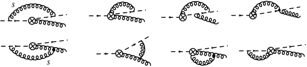
Figure 5: One-loop diagrams required for renormalization of the three-particle SCET_I operator. As before, soft gluon lines indicated by an index $s$. The wave function renormalization diagram is not shown for simplicity.

The operator RG equation reads

$$\mu\frac{d}{d\mu}O_{R}[\tau]=-\int d\tau^{\prime}\gamma[\tau,\tau^{\prime}]~{}O_{R}[\tau^{\prime}],$$

with the evolution kernel $\gamma[\tau,\tau^{\prime}]$:

$$\gamma[\tau,\tau^{\prime}]=\left\{-~{}\delta(\tau-\tau^{\prime})\Gamma_{\text{cusp}}[\alpha_{s}]\ln\left(\frac{{\mu}^{2}}{Q^{2}}\right)+\frac{\alpha_{s}}{\pi}V[\tau,\tau^{\prime}]\right\},$$ (102)

where (c.f. Chay:2005rz )

$$V[\tau,\tau^{\prime}]= ~{}-\delta(\tau-\tau^{\prime})\left(C_{F}\left[\frac{5}{2}-\ln\bar{\tau}\right]+\frac{C_{A}}{2}\ln\frac{\bar{\tau}}{\tau}\right)-\frac{C_{A}}{2}\left[\frac{\theta(\tau<\tau^{\prime})}{\left(\tau^{\prime}-\tau\right)}+\frac{\theta(\tau^{\prime}<\tau)}{\left(\tau-\tau^{\prime}\right)}\right]_{+}$$

$$+\left(C_{F}-\frac{C_{A}}{2}\right)~{}\left[\frac{\tau^{\prime}}{\bar{\tau}^{\prime}}~{}\theta(\tau^{\prime}<\bar{\tau})+\theta(\bar{\tau}<\tau^{\prime})\frac{\bar{\tau}}{\tau}\right]+~{}C_{F}~{}\bar{\tau}$$

$$-\frac{C_{A}}{2}\left[\theta(\tau<\tau^{\prime})\frac{\bar{\tau}}{\tau^{\prime}}\left(\frac{\tau^{\prime}}{\bar{\tau}}-\frac{3}{2}\right)+\theta(\tau^{\prime}<\tau)\frac{\bar{\tau}}{\bar{\tau}^{\prime}}\left(\frac{3}{2}-\frac{\bar{\tau}^{\prime}}{\tau}-\frac{1}{\bar{\tau}}\right)\right],$$ (103)

where the prescription $[...]_{+}$ is defined for the symmetrical kernel $f(\tau,\tau^{\prime})=f(\tau^{\prime},\tau)$ as

$$\left[f(\tau,\tau^{\prime})\right]_{+}=\int\tau^{\prime}f(\tau,\tau^{\prime})\left[\phi(\tau^{\prime})-\phi(\tau)\right].$$

Computing the convolution integral with the LO $C_{B}[\tau]=1$ yields the well defined expression:

$$\int_{0}^{1}d\tau^{\prime}V[\tau^{\prime},\tau]=-\left[2C_{F}-\frac{3}{8}C_{A}\right]=-\gamma_{B},$$ (104)

which does not depend on $\tau$. Hence we can conclude that the leading logarithmic convolution integral in Eq. (89) is also well defined.

The corresponding RG equation for the coefficient function reads:

$$\mu\frac{d}{d\mu}C_{B}(\tau,Q;\mu)=-\Gamma_{\text{cusp}}[\alpha_{s}]\ln\left(\frac{{\mu}^{2}}{Q^{2}}\right)C_{B}(\tau,Q;\mu)+\frac{\alpha_{s}}{\pi}\int_{0}^{1}d\tau^{\prime}~{}V[\tau^{\prime},\tau]C_{B}(\tau^{\prime},Q;\mu)~{}.$$ (105)

Similar equations have been studied already in heavy-light decays (see, e.g., Refs. HillB2004 ; Beneke:2005gs ). The NLL solution of this equation can be written as

$$C_{B}^{\text{NLL}}(\tau,Q;\mu)=e^{-S(Q;\mu_{h},\mu)}\int_{0}^{1}d\tau^{\prime}U\left[\tau,\tau^{\prime};\mu_{h},\mu\right]C_{B}^{(0)}(\tau^{\prime},Q;\mu_{h}),$$ (106)

where the evolution kernel satisfies the integro-differential equation

$$\mu\frac{d}{d\mu}U\left[\tau,\tau^{\prime};\mu_{h},\mu\right]=\frac{\alpha_{s}}{\pi}\int_{0}^{1}d\tau^{\prime\prime}~{}V[\tau^{\prime\prime},\tau]U\left[\tau^{\prime\prime},\tau^{\prime};\mu_{h},\mu\right]$$ (107)

with initial condition $U\left[\tau,\tau^{\prime};\mu_{h},\mu_{h}\right]=\delta(\tau-\tau^{\prime}).~{}$Recall that, in order to sum the large logarithms the initial scale $\mu_{h}$ should be of order $Q$, and the evolution ends at $\mu$ of order $(\Lambda Q)^{1/2}$. The Sudakov factor $S(Q;\mu_{h},\mu)$ is the same as in Eq. (99). Taking into account that at NLL approximation the initial condition $C_{B}^{(0)}(\tau^{\prime},Q;\mu_{h})$ is given by the tree-level expression Eq. (92), one can perform the integration over $\tau^{\prime}$ in Eq.(106), yielding :

$$C_{B}^{\text{NLL}}(\tau,Q,\mu)=e^{-S(Q;\mu_{h},\mu)}U_{B}\left[\tau~{};\mu_{h},\mu\right],$$ (108)

with

$$\mu\frac{d}{d\mu}U_{B}\left[\tau;\mu_{h},\mu\right]=\frac{\alpha_{s}}{\pi}\int_{0}^{1}d\tau^{\prime}~{}V[\tau^{\prime},\tau]U_{B}\left[\tau^{\prime};\mu_{h},\mu\right]$$ (109)

and $U_{B}\left[\tau;\mu_{h},\mu_{h}\right]=1$. The solution of this equation can be found numerically. We have found that to a very good accuracy the approximate solution can be written as

$$U_{B}\left[\tau;\mu_{h},\mu\right]\approx U^{\text{app}}_{B}\left[\mu_{h},\mu\right]=\left(\frac{\ln[\mu_{h}/\Lambda^{(n_{f})}]}{\ln[\mu/\Lambda^{(n_{f})}]}\right)^{2\gamma_{B}/\beta_{0}}$$ (110)

with effective anomalous dimension $\gamma_{B}$ defined in Eq.(104) and with soft scale $\Lambda^{(n_{f})}$ used for calculating the running coupling $\alpha_{s}$. To avoid confusion let us note that the soft scale $\Lambda$ which we used to define the hard-collinear scale $\sim Q\Lambda$ is different $\Lambda\neq\Lambda^{(n_{f})}$. This difference provides the slow dependence on $Q$ in the approximate solution of Eq. (110). In Fig. 6

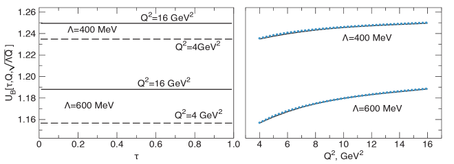
Figure 6: Left panel: numerical evaluation of the evolution kernel $U_{B}[\tau,Q,\sqrt{Q\Lambda}]$ as a function of $\tau$ at fixed $Q^{2}$. Right panel: $U_{B}[\tau,Q,\sqrt{Q\Lambda}]$ as a function of $Q$ at fixed $\tau=0.5$ for two different values of $\Lambda$ (solid curves). The approximate solution $U^{\text{app}}_{B}\left[\mu_{h},\mu\right]$ of Eq. (110) is shown by dotted (blue) curves.

we show $U_{B}\left[\tau~{};Q,\sqrt{Q\Lambda}\right]$ computed for different values of $Q$ and $\Lambda$ and compare it with the approximate solution $U^{\text{app}}_{B}$. We obtained that for all considered cases to a very good accuracy the kernel does not depend on the momentum fraction $\tau$ and evolves quite slowly with respect to $Q$ according to (110). At the end let us note that the similar approximate solution for the single-logarithmic evolution was also found for the heavy-light current in Ref. Beneke:2005gs .

The obtained results already lead to some qualitative features when applying this formalism to the proton FFs, as will be discussed in the next section.

IV QCD factorization at leading order using the SCET approach

In this section, we consider the matching on SCET_II and discuss the factorization formula for the soft rescattering mechanism. We perform an analysis of the dominant regions using the methods of the effective theory. We restrict our consideration only to the terms relevant at leading logarithmic approximation both at SCET_I and SCET_II levels. The general, all order analysis is much more complicated and goes beyond our present considerations. However, using the results obtained above, we suggest a leading order factorization formula (i.e. restricted by leading logarithms) for the Dirac FF $F_{1}$ which includes soft and hard rescattering contributions.

In this section we would like to demonstrate that the soft rescattering contribution can be estimated in SCET using the counting rules (73-75) without direct calculation of the diagrams as we did before. Such counting is an important ingredient of a factorization proof and can be considered as a quite general argument in support of the nontrivial soft rescattering contribution.

In addition to the field relations, we also need the counting of the energetic (collinear) hadronic state. It reads

$$\left|p_{c}\right\rangle\sim\lambda^{-2},$$ (111)

and follows from the conventional normalization (13).

Let us start from the well known hard rescattering picture. From existing results one can easily obtain:

$$\left\langle p^{\prime}\left|J_{\bot}^{\mu}\right|p\right\rangle\overset{Q\rightarrow\infty}{\sim}\bar{N}^{\prime}\gamma_{\bot}^{\mu}N~{}F_{1}\sim\bar{N}^{\prime}\gamma_{\bot}^{\mu}N\frac{f_{N}^{~{}2}}{Q^{4}}\sim~{}\bar{N}^{\prime}\gamma_{\bot}^{\mu}N~{}\lambda^{8},$$ (112)

and

$$\left\langle p^{\prime},\lambda^{\prime}\left|~{}J_{\|}^{\mu}\right|p,\lambda\right\rangle=\frac{(p+p^{\prime})^{\mu}}{m_{N}}~{}\bar{N}^{\prime}\hat{1}N~{}F_{2}(Q^{2})\overset{Q\rightarrow\infty}{\sim}\frac{Q}{m_{N}}~{}\frac{f_{N}^{2}~{}m_{N}^{2}}{Q^{6}}~{}\bar{N}^{\prime}\hat{1}N~{}\sim\bar{N}^{\prime}\hat{1}N~{}\lambda^{10}.$$ (113)

where the nonperturbative scale is presented by the nucleon mass $m_{N}\sim\Lambda$ and the overall normalization constant for the nucleon distribution amplitude$f_{N}\sim\Lambda^{2}$.

The same counting in SCET is obtained directly from the dimensional analysis of the leading operators constructed from the collinear and soft fields, which represent the main degrees of freedom of SCET_II. However, difficulties arise due to nonlocal contributions with inverse powers of $1/\Lambda$ momenta if one computes time-ordered products involving SCET_I fields. We shall follow the strategy suggested in Refs. Bauer:2002aj ; Bauer:2003mga . Then matching onto SCET_II,

$$\text{SCET}_{I}\left[p_{hc}^{2}\sim Q\Lambda,~{}k_{s}^{2}\sim\Lambda^{2}\right]\overset{\mu^{2}\sim Q\Lambda}{\longrightarrow}\text{SCET}_{II}\left[p_{c}^{2}\sim\Lambda^{2},~{}k_{s}^{2}\sim\Lambda^{2}\right]$$ (114)

can be performed in two steps: decoupling the soft fields from the hard collinear modes using field redefinitions expressed by Eq. (80), and subsequently matching hard-collinear modes to collinear ones

$$\{\xi_{hc}^{\prime(0)},~{}A_{hc}^{\prime(0)},\xi_{hc}^{(0)},~{}A_{hc}^{(0)}\}\rightarrow\{\xi_{c}^{\prime},~{}A_{c}^{\prime},\xi_{c},~{}A_{c}\},$$ (115)

lowering the off-shellness of the external hard-collinear fields. Notice that the last step changes the power counting of the fields from Eq. (73) to Eq. (74).

In the case of the hard rescattering we perform the matching of QCD directly onto SCET_II. Therefore, the power counting is simple because it does not involve the intermediate effective theory.

Matching for the Dirac FF $F_{1}$ involves the six-quark operator constructed only from the collinear fields $\xi_{c}^{\prime}$, $\xi_{c}$ and Wilson lines with longitudinal collinear gluons $\bar{n}\cdot A^{\prime}$ and $n\cdot A$ respectively. It is the product of two twist-3  3-quark operators which define the leading twist nucleon DA (14). Then using (74) one obtains

$$\left\langle p^{\prime}\left|J_{\bot}^{\mu}\right|p\right\rangle^{(h)}\sim\left\langle p^{\prime}\left|\bar{\xi}_{c}^{\prime}\bar{\xi}_{c}^{\prime}\bar{\xi}_{c}^{\prime}|0\left\rangle\ast C_{\bot}^{\mu}(Q)\ast\right\langle 0|\xi_{c}\xi_{c}\xi_{c}\right|p\right\rangle\sim\lambda^{8}~{}\bar{N}^{\prime}\gamma_{\bot}^{\mu}N.$$ (116)

For the helicity flip FF $F_{2}$, the matching involves the product of twist-3 and twist-4 operators, as we discussed in Sec. III. Schematically this situation can be described by substituting $\xi_{c}\rightarrow\eta_{c}\sim\xi_{c}/Q$. Then

$$\left\langle p^{\prime}\left|J_{\|}^{\mu}\right|p\right\rangle^{(h)}\sim\left\langle p^{\prime}\left|\bar{\xi}_{c}^{\prime}\bar{\xi}_{c}^{\prime}\bar{\xi}_{c}^{\prime}|0\left\rangle\ast C_{\|}^{\mu}(Q)\ast\right\langle 0|\eta_{c}\xi_{c}\xi_{c}\right|p\right\rangle \sim(n+\bar{n})^{\mu}~{}\lambda^{10}~{}\bar{N}^{\prime}\hat{1}N$$ (117)

$$\sim\lambda^{12}~{}\frac{(p+p^{\prime})^{\mu}}{m}\bar{N}^{\prime}\hat{1}N~{},$$ (118)

and we obtain that $F_{2}$ is suppressed as $1/Q^{2}$ relative to $F_{1}$ as it should be.

In order to estimate the soft rescattering contribution one has to perform a more complicated analysis with the two-step matching: QCD$\rightarrow$SCET_I $\rightarrow$SCET_II.  The matching onto SCET_I has been done in Section IV and for the electromagnetic current at leading order it yields the formula Eq. (89).  In matching onto SCET_II we need at least six collinear quarks in order to have overlap with the in and out nucleon states. Next, guided by the perturbative QCD calculations from Sec. II we need higher order vertices $\mathcal{L}_{\xi q}^{(n)}$ in order to describe the soft spectators in the intermediate state.

IV.1 Leading-order SCET analysis for Dirac FF $F_{1}$

Let us start with a discussion for the FF $F_{1}$. To leading order in $1/Q$ we can restrict our consideration by the first term in Eq. (89). Therefore our task is to compute the time-ordered product which contributes to the matrix element

$$\left\langle p^{\prime}\left|J_{\bot}^{\mu}~{}(0)\right|p\right\rangle^{(s)}\simeq\left\langle p^{\prime}\right|~{}T\left\{C_{A}~{}O_{A}^{\mu_{\bot}}~{}e^{i\mathcal{L}^{(\bar{n})}_{\text{SCET}_{I}}+i\mathcal{L}^{(n)}_{\text{SCET}_{I}}+i\mathcal{L}_{s}}\right\}~{}\left|p\right\rangle.$$ (119)

The calculations amount to integrating out hard-collinear modes and, if possible, to deriving the expression for the vector current $J_{\bot}^{\mu}$ in terms of SCET_II collinear and soft fields which can be schematically written as

$$T\left\{C_{A}O_{A}^{{\mu}_{\bot}}~{}e^{i\mathcal{L}^{(\bar{n})}_{\text{SCET}_{I}}+i\mathcal{L}^{(n)}_{\text{SCET}_{I}}+i\mathcal{L}_{s}}\right\}$$

$$\simeq C_{A}\text{\bf Tr}\left[\gamma^{\mu}_{\bot}\,T\left\{\mathbf{O}_{out}\left(\varphi_{c}^{\prime}\right)~{}e^{i\mathcal{L}_{c}^{(\bar{n})}}\right\}\ast\mathbf{J}^{\prime}\ast T\left\{\mathbf{S}\left(\varphi_{s}\right)~{}e^{i\mathcal{L}_{s}}\right\}\ast\mathbf{J}\ast T\left\{\mathbf{O}_{in}\left(\varphi_{c}\right)~{}e^{i\mathcal{L}_{c}^{({n})}}\right\}\,\right],$$ (120)

where $\mathbf{J}$ and $\mathbf{J}^{\prime}$ are jet functions, $\mathcal{L}_{c}^{(n)}$ denotes the collinear Lagrangian, Tr denotes contractions over the Dirac and color indices which are not shown explicitly, and where we used the notation $\varphi_{c,s}\equiv\{\xi_{c,s},A_{c,s}\}$. We also assumed that the collinear operators $\mathbf{O}_{in,out}$ have nontrivial overlap with nucleon states. The Dirac matrix $\gamma^{\mu}_{\bot}$ is associated with the vertex of the $O_{A}$ operator. It is clear that the existence of the factorized representation (120) is equivalent to establishing the factorization theorem. Guided by our QCD analysis, carried out in Sec. II, we demonstrate below that at leading order in $1/Q$ such a contribution definitely exists. For simplicity, we restrict our consideration to a leading-order analysis in $\alpha_{s}$, and consider it as a first step towards a complete proof.

Obviously, the time-ordered product in left hand side of (120) can be represented as the product of two:

$$T\left\{...\right\}=T\left(\bar{\xi}_{hc}^{\prime}W^{\prime}(0)~{}e^{i\mathcal{L}^{(\bar{n})}_{\text{SCET}_{I}}}~{}\right)\gamma_{\bot}^{\mu}~{}T\left(W\xi_{hc}(0)~{}e^{i\mathcal{L}^{(n)}_{\text{SCET}_{I}}}\right)\equiv T_{out}~{}\gamma_{\bot}^{\mu}~{}T_{in}$$ (121)

where we “freeze” the soft fields, i.e., consider them as external. As calculations of the each of the $T$ products are almost identical, we only consider one of them. The result of the integration over hard-collinear modes can be schematically written as

$$T_{out}=T\left(\bar{\xi}_{hc}^{\prime}W^{\prime}~{}e^{i\mathcal{L}^{(\bar{n})}_{\text{SCET}_{I}}}~{}\right)\ \simeq\mathbf{~{}~{}}\bar{\xi}_{c}^{\prime}\bar{\xi}_{c}^{\prime}\bar{\xi}_{c}^{\prime}\ast\mathbf{J}^{\prime}\ast qq~{},\ \ \$$ (122)

where the last equation shows the desired structure in terms of collinear and soft fields. Combining such results for $T_{in}$ and $T_{out}$ we obtain desired representation (120).

Let us now consider in details the calculation of the right-hand side of Eq.(122). The relevant $T$ product is of order $\lambda^{3}$ and to leading order in $\alpha_{s}$ reads

$$T_{out}\equiv T_{out}^{(3)}\simeq\int d^{4}x_{1}\int d^{4}x_{2}\int d^{4}x_{3}~{}T\left(\bar{\xi}_{hc}^{\prime}W^{\prime}(0),\mathcal{L}_{\xi q}^{(1)}(x_{1}),\mathcal{L}_{\xi q}^{(1)}(x_{2}),\mathcal{L}_{\xi}^{(0)}(x_{3})\right),$$ (123)

where $\mathcal{L}_{\xi q}^{(1)}$ is the leading-order soft-collinear contribution in Eq. (78). We did not find the other possibilities to obtain the leading in the $1/Q$ result. Time-ordered products with insertions of other higher order contributions $\mathcal{L}_{\xi q}^{(n)}$ with $n\geq 2$ from the collinear or soft-collinear sectors can provide only suppressed operators in SCET_II and therefore can be excluded from the consideration. Performing a decoupling of the soft field with the help of Eq. (80) we obtain

$$\bar{\xi}_{hc}^{\prime}W^{\prime}(0)\rightarrow\bar{\xi}_{hc}^{\prime(0)}W^{\prime}(0)S_{n}^{{\dagger}}(0),~{}\mathcal{L}_{\xi q}^{(1)}(x)\rightarrow\bar{\xi}_{hc}^{\prime(0)}~{}i\hat{D}_{\bot}W~{}\left[S_{n}^{{\dagger}}(x_{-})q(x_{-})\right].\ \$$ (124)

The eikonal factors $S_{n}^{{\dagger}}$ ensure the gauge invariance of the soft sector described by the soft quark fields. Subsequently, we compute the contractions of the hard-collinear fields which can be conveniently presented by Feynman graphs. The leading-order contribution to $T_{out}^{(3)}$ is given by the set of diagrams shown in Fig.7.

Figure 7: Leading-order SCET diagrams required for the calculation of jet functions. The inner dashed and curly lines denote hard-collinear quarks and gluons, external dashed lines correspond to collinear quarks, fermion lines with crosses denote soft quarks. Black squares denote the vertex of the SCET_I operator.

Note that the last two diagrams with the three-gluon vertex have zero color factor and therefore do not contribute. This is in full agreement with the similar observation made in Ref. Fadin1981 . The remaining diagrams have a similar topology and the corresponding power counting can be easily established. The contractions of the hard-collinear fields yield

$$\int d^{4}x_{1}~{}\left\langle A_{hc\bot}^{\alpha}(x_{1})A_{hc\bot}^{\beta}(x_{2})\right\rangle\sim\int d^{4}x_{2}~{}\left\langle(\bar{n}\cdot A_{hc})(x_{2})(n\cdot A_{hc})(x_{3})\right\rangle\sim\lambda^{-2},$$ (125)

$$\int d^{4}x_{3}\left\langle~{}\bar{\xi}_{hc}(x_{1})\xi_{hc}(x_{3})\right\rangle\sim\lambda^{-2},$$ (126)

i.e., all hard-collinear contractions cost $\lambda^{-2}$, which results from the hard-collinear propagators in momentum space. Remember that we assume that external hard-collinear particles are matched onto collinear ones. Therefore taking into account the external collinear and soft fields we obtain

$$T_{out}^{(3)}\sim\underset{\text{h-coll contractions}}{\underbrace{\lambda^{-2}\lambda^{-2}\lambda^{-2}}\ }\times\underset{\text{2 soft fields}}{\underbrace{\lambda^{3}\lambda^{3}}}\times\underset{\text{3 coll fields}}{\underbrace{\lambda^{2}\lambda^{2}\lambda^{2}}}~{}\sim\lambda^{6}.$$ (127)

The same counting is also relevant for the second time-ordered product in Eq. (121). Therefore the order of the total contribution in SCET_II now reads

$$\left\langle p^{\prime}\left|~{}J_{\bot}^{\mu}\right|p\right\rangle_{(s)}\sim T_{out}^{(3)}\times T_{in}^{(3)}\times\lambda^{-4}~{}~{}\bar{N}^{\prime}\gamma_{\bot}^{\mu}N\sim\lambda^{8}~{}\bar{N}^{\prime}\gamma_{\bot}^{\mu}N.$$ (128)

We observe that the soft rescattering contribution has the same power suppression as the hard one [ Eq. (116)].

Let us briefly discuss the general structure of the soft rescattering contribution. It is clear from the above consideration that the leading-order jet functions can be computed from the diagrams in Fig. 7. The details of their calculations and explicit expressions will be presented in a different publication inprep . From the QCD calculation, we noticed that at tree level the transverse momentum is completely defined by external soft and collinear fields and therefore it scales as $k_{\bot}\sim Q\lambda^{2}$. Such counting ratio remains true for the hard-collinear lines inside diagrams due to the momentum conservation. Therefore the transverse components in the hard-collinear propagators (for tree diagrams only!) can be neglected. Consequently, the arguments of the external collinear and soft fields are local in transverse space and depend only on the relevant light-cone components. In SCET the same properties follow from the multipole expansion of the fields with respect to the small parameter $\lambda$. Therefore computing the diagrams in Fig. 7 and passing to momentum space one obtains

$$T_{out}^{(3)}\simeq\int Dy_{i}\boldsymbol{O}_{out}(y_{i})\,\int d\omega_{1,2}~{}\mathbf{J}^{\prime}\left(y_{i},\omega_{i}Q\right)\,\boldsymbol{S}_{n}(\omega_{i}),$$ (129)

with the following collinear and soft operators:

$$\boldsymbol{O}_{out}(y_{i})=4~{}\prod_{i=1}^{3}\int\frac{d\hat{z}_{i}^{+}}{2\pi} e^{-\frac{i}{2}\left({P}^{\prime}\cdot\bar{n}\right)\left(y_{1}z_{1}^{+}+y_{2}z_{2}^{+}+y_{3}z_{3}^{+}\right)}$$ (130)

$$\times\varepsilon^{ijk}~{}\bar{\xi}_{c}^{\prime}W_{c}^{\prime i}({{\scriptstyle\frac{1}{2}}}z_{1}^{+}~{}\bar{n})~{}\bar{\xi}_{c}^{\prime}W_{c}^{\prime j}({{\scriptstyle\frac{1}{2}}}z_{2}^{+}~{}\bar{n})~{}\bar{\xi}_{c}^{\prime}W_{c}^{\prime k}({{\scriptstyle\frac{1}{2}}}z_{3}^{+}~{}\bar{n}),$$

and

$$\boldsymbol{S}_{n}(\omega_{i})=\varepsilon^{i^{\prime}j^{\prime}k^{\prime}}\int\frac{dz_{1,2}^{-}}{2\pi}e^{\frac{i}{2}(\omega_{1}z_{1}^{-}+\omega_{2}z_{2}^{-})}\left[S_{n}^{{\dagger}}(0)\right]^{k^{\prime}l}\left[S_{n}^{{\dagger}}\frac{\hbox to0.0pt{\hbox to5.00002pt{\hfil$\bar{n}$\hfil}\hss}/\hbox to0.0pt{\hbox to6.00235pt{\hfil/\hfil}\hss}n}{4}q({{\scriptstyle\frac{1}{2}}}z_{1}^{-}n)\right]^{j^{\prime}}\left[S_{n}^{{\dagger}}\frac{\hbox to0.0pt{\hbox to5.00002pt{\hfil$\bar{n}$\hfil}\hss}/\hbox to0.0pt{\hbox to6.00235pt{\hfil/\hfil}\hss}n}{4}q({{\scriptstyle\frac{1}{2}}}z_{2}^{-}n)\right]^{k^{\prime}}$$ (131)

where we do not show for simplicity the spinor indices, ${P}^{\prime}$ denotes the total collinear momentum operator, $z_{i}^{-}\equiv(z_{i}\cdot\bar{n})$, $z_{i}^{+}\equiv(z_{i}\cdot n)$, and $d\hat{z}_{i}^{+}\equiv d{z}_{i}^{+}Q$. The structure for $T_{in}^{(3)}$ can be obtained in an analogous way. Combining these results we obtain operator expression with structure (120) which schematically can be written as

$$T\{C_{A}O_{A}^{{\mu}_{\bot}}\}\simeq C_{A}\,\text{\bf Tr}\left[\,\gamma^{\mu}_{\bot}\mathbf{O}_{out}(y_{i})\ast\mathbf{J}^{\prime}\left[y_{i},\omega_{i}Q\right]\ast\left\{\mathbf{S}_{\bar{n}}~{}\mathbf{S}_{n}\right\}\ast\mathbf{J}[x_{i},\nu_{i}Q]\ast\mathbf{O}_{in}(x_{i})\,\right].$$ (132)

Substituting these results into the matrix element of Eq. (119) and taking account of the decoupling of the collinear and soft modes (see, e.g., Bauer2001 ; Bauer:2003mga ) one obtains three matrix elements: two with the collinear fields and the soft correlation function. The collinear matrix elements can be easily converted into DAs (14):

$$\int Dy_{i}\left\langle p^{\prime}\right|\boldsymbol{O}_{out}(y_{i})\left|0\right\rangle~{}\mathbf{J}^{\prime}(y_{i},\omega_{i}Q)=\int Dy_{i}~{}~{}\mathbf{\Psi}^{\prime}(y_{i})~{}\mathbf{J}^{\prime}(y_{i},\omega_{i}Q).$$ (133)

Rewriting the initial matrix element $\left\langle 0\right|~{}\xi_{c}\xi_{c}\xi_{c}\left|p\right\rangle\sim\mathbf{\Psi}$ in the same way and combining all contributions, we obtain the factorization formula for the soft rescattering contribution:

$$F_{1}^{(s)}(Q^{2}) \simeq C_{A}(Q,\mu_{I})\int Dy_{i}\mathbf{\Psi}^{\prime}(y_{i},\mu_{II})\int_{0}^{\infty}d\omega_{1}d\omega_{2}~{}\mathbf{J}^{\prime}(y_{i},\omega_{i}Q,\mu_{I},\mu_{II})$$ (134)

$$\times\int Dx_{i}\mathbf{\Psi}(x_{i},\mu_{II})\int_{0}^{\infty}d\nu_{1}d\nu_{2}~{}\mathbf{J}(x_{i},\nu_{i}Q,\mu_{I},\mu_{II})\boldsymbol{S}(\omega_{i},\nu_{i};\mu_{II}),$$

where the soft correlation function is defined as

$$~{}\boldsymbol{S}(\omega_{i},\nu_{i};\mu_{II})=\int\frac{d\eta_{1}}{2\pi}\int\frac{d\eta_{2}}{2\pi}~{}e^{-i\eta_{1}\nu_{1}-i\eta_{2}\nu_{2}}\int\frac{d\lambda_{1}}{2\pi}\int\frac{d\lambda_{2}}{2\pi}e^{i\lambda_{1}\omega_{1}+i\lambda_{2}\omega_{2}}\left\langle 0\right|\mathbf{O}_{S}(\eta_{i},\lambda_{i})\left|0\right\rangle,$$ (135)

with the operator

$$\mathbf{O}_{S}(\eta_{i},\lambda_{i}) = \varepsilon^{i^{\prime}j^{\prime}k^{\prime}}\left[S_{n}^{{\dagger}}(0)\right]^{i^{\prime}l}\left[S_{n}^{{\dagger}}\frac{\hbox to0.0pt{\hbox to5.00002pt{\hfil$\bar{n}$\hfil}\hss}/\hbox to0.0pt{\hbox to6.00235pt{\hfil/\hfil}\hss}n}{4}q(\lambda_{1}n)\right]_{\sigma}^{j^{\prime}}\left[S_{n}^{{\dagger}}\frac{\hbox to0.0pt{\hbox to5.00002pt{\hfil$\bar{n}$\hfil}\hss}/\hbox to0.0pt{\hbox to6.00235pt{\hfil/\hfil}\hss}n}{4}q(\lambda_{2}n)\right]_{\rho}^{k^{\prime}}$$ (136)

$$\times \varepsilon^{ijk}\left[S_{\bar{n}}(0)\right]^{li}\left[\bar{q}\frac{\hbox to0.0pt{\hbox to5.00002pt{\hfil$\bar{n}$\hfil}\hss}/\hbox to0.0pt{\hbox to6.00235pt{\hfil/\hfil}\hss}n}{4}S_{\bar{n}}(\eta_{1}\bar{n})\right]_{\alpha}^{j}\left[\bar{q}\frac{\hbox to0.0pt{\hbox to5.00002pt{\hfil$\bar{n}$\hfil}\hss}/\hbox to0.0pt{\hbox to6.00235pt{\hfil/\hfil}\hss}n}{4}S_{\bar{n}}(\eta_{2}\bar{n})\right]_{\beta}^{k},$$

which is shown graphically in Fig. 8.

Figure 8: Graphical representation of the operator of Eq. (136) entering the soft correlation function. Dashed and dotted lines denote the different light-cone directions.

In the last equation we assume $\bar{q}S_{\bar{n}}(\eta_{2}\bar{n})=\bar{q}(\eta_{2}\bar{n})S_{\bar{n}}(\eta_{2}\bar{n})$, and the color and Dirac indices are shown explicitly. Furthermore in Eq. (134), $C_{A}$ denotes the hard coefficient function which has been computed in the leading-order approximation (92).

In Eq. (134) we show explicitly two factorization scales $\mu_{I}$ and $\mu_{II}$ . The total contribution, as usually, does not depend on these auxiliary quantities. The first scale $\mu_{I}$ arises at the matching QCD to SCET_I. The evolution equations at leading logarithmic approximation with respect to $\mu_{I}$ were discussed above. In practical applications it is convenient to fix this scale at the value $\mu_{I}^{2}\simeq\Lambda Q$. Then the large logarithms $\ln[Q^{2}/\mu_{I}^{2}$] can be resummed solving RG equations. The second scale $\mu_{II}$ appears when one performs the second reduction to SCET_II. Usually, the corresponding coefficient functions ( = jet functions $J^{\prime}$ and $J$ ) are computed at $\mu_{II}^{2}\simeq$ $\Lambda Q$ and then the scale is fixed to be $\mu_{II}^{2}\simeq$ $\Lambda^{2}$.  Again, arising large logarithms $\ln[Q\Lambda/\mu_{II}^{2}]$ must be resummed with the help of evolution equations for nucleon DAs $\mathbf{\Psi}(x_{i},\mu_{II})$ and CF $\boldsymbol{S}(\omega_{i},\nu_{i},\mu_{II})$. The evolution of the DAs is well studied in the literature (see, e.g. Refs. Chernyak:1983ej ; Lepage:1979zb and Braun:1999te for recent progress ) but the corresponding equation for $\boldsymbol{S}(\omega_{i},\nu_{i},\mu_{II})$ is new and has not been derived before. Such a calculation must be done because it will provide an important check of the factorization formula (134) at leading logarithmic accuracy. A derivation of the jet functions and evolution kernel for $\boldsymbol{S}(\omega_{i},\nu_{i},\mu)$ will be presented in a separate publication inprep . In the Appendix B to this paper we demonstrate how the perturbative QCD result of Eq. (48) is reproduced from the corresponding SCET diagram in Fig.7.

It turns out that the product of the nucleon DA and jet function has the same Dirac and color structure as $~{}\mathbf{\Psi}^{\prime}(y_{i})$ (16):

$$~{}\mathbf{J}(x_{i},\omega_{i})~{}\mathbf{\Psi}(x_{i}) =~{}\Omega_{V}(x_{i},\omega_{i})~{}~{}p_{+}\left[{\scriptstyle\frac{1}{2}}\hbox to0.0pt{\hbox to5.00002pt{\hfil/\hfil}\hss}\bar{n}~{}C\right]_{\alpha\beta}\left[\gamma_{5}N^{+}\right]_{\sigma}$$

$$+~{}\Omega_{A}(x_{i},\omega_{i})~{}~{}p_{+}\left[{\scriptstyle\frac{1}{2}}\hbox to0.0pt{\hbox to5.00002pt{\hfil/\hfil}\hss}\bar{n}\gamma_{5}C\right]_{\alpha\beta}\left[N^{+}\right]_{\sigma}$$ (137)

$$\ +\Omega_{T}(x_{i},\omega_{i})~{}p_{+}\left[{\scriptstyle\frac{1}{2}}\hbox to0.0pt{\hbox to5.00002pt{\hfil/\hfil}\hss}\bar{n}\gamma_{\bot}C\right]_{\alpha\beta}\left[\gamma^{\bot}\gamma_{5}N^{+}\right]_{\sigma}.$$

where the coefficients  $\Omega_{X}(x_{i},\omega_{i})$ are linear combinations of the nucleon DAs (16) and hard-collinear jet functions

$$~{}\Omega_{X}(x_{i},\omega_{i})=J_{XV}(x_{i},\omega_{i})V(x_{i})+J_{XA}(x_{i},\omega_{i})A(x_{i})+J_{XT}(x_{i},\omega_{i})T(x_{i}).$$ (138)

Therefore, the jet function can be interpreted as a hard-collinear component of the three-quark nucleon wave function describing the transition of the three collinear quark state into configuration with one hard-collinear and two soft quarks. Correspondingly, the CF $\boldsymbol{S}(\omega_{i},\nu_{i},\mu_{II})$ (135) describes the propagation of the soft diquark state in the background of the soft-gluon field created by a fast moving active quark: i.e., it describes the soft overlap of the nucleon wave function. Therefore we expect that the soft rescattering picture can also be associated with the well known mechanism, suggested by Feynman a long time ago Feynman:1973xc .

In the factorization formula of Eq. (134) we restricted the fractions $\omega_{i}$ and $\nu_{i}$ to be defined on the real semiaxis, assuming that all the functions in (134) are real functions. This allows us to avoid the poles in the propagators of the tree diagrams in Fig. 7 and ensures that the jet functions are real. Recall, that the reality of the nucleon form factors is guaranteed by the time reversal invariance of QCD.

The other interesting observation which follows already from the QCD computation (48) is the absence of the end-points singularities in the convolution integrals of DAs with jet functions in Eq. (137). Let us assume that the convolution integrals with respect to the soft fractions $\omega_{i},\nu_{i}$ in (134) are also well defined. Then this allows us to suggest that hard rescattering and the soft rescattering mechanisms provide additive contributions to the total FF $F_{1}$ at least to leading logarithmic accuracy:

$$F_{1}\simeq F_{1}^{(s)}+F_{1}^{(h)},$$ (139)

with the well known expression for the hard rescattering part: $F_{1}^{(h)}=\mathbf{\Psi}\ast\mathbf{H}\ast\mathbf{\Psi}$. Recall that the convolution integrals for $F_{1}^{(h)}$ at leading logarithmic accuracy are also well defined. Hence we may conclude that there is no double counting in this case. The formula of Eq. (139), together with the result of Eq. (134), is our suggestion for the full factorization formula for the Dirac FF at large $Q^{2}$. We would like to emphasize that the obtained results have been derived at leading order and only partially verified at the leading logarithmic approximation. A discussion of an all order factorization proof for Eqs. (134) and (139) requires more detailed analysis and goes beyond this publication.

IV.2 Leading order SCET analysis for Pauli FF $F_{2}$

In contrast to $F_{1}$, the description of the Pauli FF $F_{2}$ is more complicated. First, it is well known that hard gluon exchange can produce large logarithms,

$$F_{2}^{(h)}=\mathbf{\Psi}\ast\mathbf{H}\ast\mathbf{\Psi}\sim\alpha_{s}^{2}\ln^{2}Q^{2}/\mu^{2},$$ (140)

which arise due to the end-point singularities in the convolution integrals Belitsky:2002kj . This is perhaps, an indication that the hard and soft rescattering mechanisms overlap. Therefore, in order to find the correct description for $F_{2}$ one has to formulate a clear recipe for how to avoid double counting in the calculation of soft and hard rescattering contributions. Such a problem for $F_{2}$, probably, arises already at the level of matching QCD to SCET_I. However, our analysis from the previous section does not show any problems with the SCET_I convolution integrals for the coefficient function $C_{B}$ [see, e.g., Eq. (104)]. Moreover, resummation of the leading Sudakov logarithms can be carried out exactly because the problematic logarithms (140) admix only at the next-to-leading accuracy. The structure of the logarithms beyond the leading order is an important subject which remains to be established for a full proof of the factorization theorem. As a first step in this direction, we demonstrate here that the SCET counting rules confirm the power suppression of the soft rescattering contribution in $F_{2}$ obtained from the QCD calculation in Sec. II.

For this purpose, the relevant part of the SCET_I vector current follows from Eq. (89) as :

$$J_{\|}^{\mu}~{}(0)=-\frac{1}{Q}\left(n^{\mu}+\bar{n}^{\mu}\right)\int_{0}^{1}d\tau~{}~{}\left(\bar{\xi}_{hc}^{\prime}W^{\prime}\right)\left[\hbox to0.0pt{\hbox to7.50002pt{\hfil/\hfil}\hss}\mathcal{A}_{\bot}^{\prime}(\tau)+\hbox to0.0pt{\hbox to7.50002pt{\hfil/\hfil}\hss}\mathcal{A}_{\bot}(\tau)\right]\left(W^{{\dagger}}\xi_{hc}\right)~{},$$ (141)

with $\hbox to0.0pt{\hbox to7.50002pt{\hfil/\hfil}\hss}\mathcal{A}_{\bot}^{\prime}(\tau)+\hbox to0.0pt{\hbox to7.50002pt{\hfil/\hfil}\hss}\mathcal{A}_{\bot}(\tau)$ as given in Eq. (91). For the qualitative discussion we consider the first term with $\hbox to0.0pt{\hbox to7.50002pt{\hfil/\hfil}\hss}\mathcal{A}_{\bot}^{\prime}$ only. Following the similar arguments as before we arrive at an analysis of time-ordered products:

$$\ \ \ \ \ \ \ \ \ \ T\left\{J_{\|}^{\mu}(0)~{}e^{i\mathcal{L}^{(\bar{n})}+i\mathcal{L}^{(n)}}\right\}=\frac{\bar{n}^{\mu}}{(\bar{n}\cdot\partial)}~{}T_{out}^{(4)}~{}T_{in}^{(3)}+\dots,$$ (142)

$$T_{out}^{(4)}= T\left\{\left(\bar{\xi}_{hc}^{\prime}W^{\prime}\right)(0)\hbox to0.0pt{\hbox to7.50002pt{\hfil/\hfil}\hss}\mathcal{A}_{\bot}^{\prime}(0)e^{i\mathcal{L}^{(\bar{n})}}\right\},~{}T_{in}^{(3)}=T\left\{\left(W^{{\dagger}}\xi_{hc}\right)(0)e^{i\mathcal{L}^{(n)}}\right\}.$$ (143)

To obtain Eq.(142) we converted (141) into position space and for simplicity wrote explicitly only the term $\sim\bar{n}^{\mu}$. The second term $T_{in}^{(3)}$ in Eq.(143) is the same as the one appearing in $F_{1}$. Hence we only have to consider the new term $T_{out}^{(4)}$. Consider the following contribution:

$$T_{out}^{(4)}\simeq T\left(\bar{\xi}_{c}^{\prime}(0)\hbox to0.0pt{\hbox to5.55557pt{\hfil/\hfil}\hss}\hat{A}_{hc\bot}^{\prime}(0)\int dx_{1}\mathcal{L}_{\xi q}^{(1)}(x_{1})\int dx_{2}\mathcal{L}_{\xi\xi}^{(0)}(x_{2})\int dx_{3}\mathcal{L}_{\xi q}^{(1)}(x_{3})\right)$$ (144)

$${\textstyle\simeq T\left(\bar{\xi}_{c}^{\prime}(0)\hbox to0.0pt{\hbox to5.55557pt{\hfil/\hfil}\hss}\hat{A}_{hc\bot}^{\prime}(0),\int dx_{1}~{}\bar{\xi}_{hc}^{\prime}A_{hc\bot}q(x_{1}),\int dx_{2}~{}\bar{\xi}_{c}^{\prime}\ \left(n\cdot A_{hc}\right)\xi_{hc}(x_{2}),\int dx_{3}~{}\bar{\eta}_{c}^{\prime}\left(\bar{n}\cdot A_{hc}\right)q(x_{3})\right),}$$ (145)

where we substituted the small component

$$\bar{\eta}_{c}^{\prime}=\bar{\xi}_{c}^{\prime}i\hbox to0.0pt{\hbox to10.00002pt{\hfil/\hfil}\hss}\overleftarrow{D}_{\bot c}(i\bar{n}\cdot\overleftarrow{D}_{c})^{-1}\frac{\hbox to0.0pt{\hbox to5.00002pt{\hfil$\bar{n}$\hfil}\hss}/}{2}\simeq\bar{\xi}_{c}^{\prime}~{}g\hat{A}_{c\bot}(i\bar{n}\cdot\overleftarrow{\partial})^{-1}\frac{\hbox to0.0pt{\hbox to5.00002pt{\hfil$\bar{n}$\hfil}\hss}/}{2}.$$ (146)

The presence of the small component $\bar{\eta}_{c}^{\prime}$ can be explained by interaction with the longitudinal photon. The outgoing collinear state must have one collinear transverse gluon or transverse derivative in order to satisfy conservation of the orbital momentum. Contracting the hard collinear fields in Eq. (145) one obtains the diagram as in Fig. 9.

Figure 9: SCET diagram for matching the quark-gluon hard-collinear state onto three collinear quarks for Pauli FF. The small component $\bar{\eta}_{c}^{\prime}$ is shown as a quark gluon state $\bar{\xi}_{c}^{\prime}A_{c\bot}$.

Using Eqs. (125) and (126) one easily obtains

$$T_{out}^{(4)}\sim\underset{\text{2 soft fileds}}{\underbrace{\lambda^{3}\lambda^{3}}}\times\underset{\text{~{}3 coll fields}}{\underbrace{\lambda^{2}\lambda^{2}\lambda^{4}}}~{}\times\underset{\text{h-coll contractions}}{\underbrace{\lambda^{-2}\lambda^{-2}\lambda^{-2}}}\sim\lambda^{8}.$$ (147)

Then the total contribution reads

$$\left\langle p^{\prime}\left|J_{\|}^{\mu}\right|p\right\rangle \sim T_{out}^{(4)}\times T_{in}^{(3)}\times\lambda^{-4}~{}(n+\bar{n})^{\mu}~{}\bar{N}~{}\hat{1}N\$$ (148)

$$\sim\lambda^{6}~{}\lambda^{8}~{}\lambda^{-4}~{}(n+\bar{n})^{\mu}~{}\bar{N}~{}\hat{1}N\sim\lambda^{10}~{}(n+\bar{n})^{\mu}~{}\bar{N}~{}\hat{1}N,$$ (149)

i.e., we obtained the same result as in the case of the hard rescattering mechanism (118). In the Appendix we demonstrate that the diagram in Fig. 9 reproduces the QCD expression for $J^{\prime}$ from Eq. (II.2). However, contrary to the Dirac FF, the convolution integral with respect to the collinear momentum fraction $\Psi^{\prime}\ast\mathbf{J}^{\prime}$ is not defined due to the end-point divergencies. Therefore we assume that the matching onto SCET_II for the Pauli FF $F_{2}$ cannot provide a well defined expression. As we discussed above, even matching onto SCET_I, one is faced with the mixing problem between hard and soft rescattering contributions.

V Phenomenological application to the nucleon FFs

In order to perform a first phenomenological analysis we introduce SCET_I form factors defined as the following nucleon matrix elements,

$$\left\langle p^{\prime}\left|\left(\bar{\xi}^{\prime}_{q}W^{\prime}\right)\gamma_{\bot}^{\mu}\left(W^{{\dagger}}\xi_{q}\right)~{}\right|p\right\rangle_{\text{SCET}_{I}}=\bar{N}(p^{\prime})\frac{\hbox to0.0pt{\hbox to5.00002pt{\hfil$\bar{n}$\hfil}\hss}/\hbox to0.0pt{\hbox to6.00235pt{\hfil/\hfil}\hss}n}{4}\gamma_{\bot}^{\mu}\frac{\hbox to0.0pt{\hbox to5.00002pt{\hfil$\bar{n}$\hfil}\hss}/\hbox to0.0pt{\hbox to6.00235pt{\hfil/\hfil}\hss}n}{4}N(p)~{}f_{1}^{q}(Q_{I},\mu)\equiv\bar{N}_{+}^{\prime}~{}\gamma_{\bot}^{\mu}N_{+}~{}f_{1}^{q}(Q_{I},\mu),$$ (150)

and

$$\left\langle p^{\prime}\left|O_{B}[\tau]~{}\right|p\right\rangle_{\text{SCET}_{I}}=~{}\bar{N}_{+}^{\prime}~{}\hat{1}~{}N_{+}(p)~{}\frac{m_{N}}{2}f_{2}^{q}(\tau;Q_{I},\mu),$$ (151)

with the operator $O_{B}[\tau]$ defined in Eq. (91). We also used the notation $Q_{I}\sim\sqrt{Q\Lambda}$ in order to stress that the defined quantities do not depend on the large scale $Q^{2}$. We indicate explicitly in the right-hand side of Eqs. (150,151) the renormalization scale dependence.

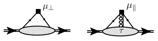
Figure 10: Graphical representation of the SCET_I FFs $f_{1}$ (left panel) and $f_{2}$ (right panel). In $f_{2}$, $\tau$ corresponds with the gluon momentum fraction.

Taking the nucleon matrix element from both sides of Eq. (89), we obtain

$$F_{1}^{(s)}(Q^{2})=C_{A}(Q,\mu_{I})\sum_{q}e_{q}~{}f_{1}^{q}(Q_{I},\mu)=C_{A}(Q,\mu)~{}f_{1}(Q_{I},\mu),$$ (152)

$$F_{2}^{(s)}(Q^{2})=\frac{m^{2}_{N}}{Q^{2}}\int_{0}^{1}d\tau~{}C_{B}(\tau,Q,\mu)\sum_{q}e_{q}~{}f_{2}^{q}(\tau;Q_{I},\mu)=\frac{m^{2}_{N}}{Q^{2}}\int_{0}^{1}d\tau~{}C_{B}(\tau,Q,\mu)~{}f_{2}(\tau;Q_{I},\mu).$$ (153)

Eqs.(152) and (153) are presented in Fig.10 in graphical form.

Using NLL approximation for the coefficient functions (98) and (108) these results can be represented as

$$F_{1}^{(s)}(Q^{2}) \simeq e^{-S(Q,\mu_{h},\mu_{I})}U_{A}~{}(\mu_{h},\mu_{I})~{}f_{1}(Q_{I},\mu_{I}),~{}\ \$$ (154)

$$F_{2}^{(s)}(Q^{2}) \simeq\frac{m^{2}_{N}}{Q^{2}}e^{-S(Q;\mu_{h},\mu_{I})}\int_{0}^{1}d\tau U_{B}\left[\tau~{};\mu_{h},\mu_{I}\right]\ f_{2}(\tau;Q_{I},\mu_{I}),~{}\$$ (155)

where the scale $\mu_{I}\simeq Q_{I}\sim\sqrt{\Lambda Q}$. From the right-hand side of Eqs. (154,155) one can see that the SCET₁ FFs $f_{1,2}$ depend now only on the hard-collinear scales. All dependence from the large scale of order $Q^{2}$ is factorized into Sudakov factors $e^{-S(Q,\mu_{h},\mu_{I})}$. This is the main feature of the Feynman mechanism. We could expect that the hard scattering contribution in $F_{1}$ provides corrections of order $\alpha_{s}^{n+2}\ln^{n}Q^{2}/\mu^{2}$ which are suppressed relative to the contributions computed in Eq. (154), and therefore can be neglected:

$$F_{1}(Q^{2})\simeq F_{1}^{(s)}(Q^{2}).$$ (156)

In the case of the Pauli FF $F_{2}$, the situation is more delicate due to a possible overlap of hard and soft rescattering terms. From the calculations of the hard scattering contribution Belitsky:2002kj , one obtains, due to the end-point singularities, contribution of order $\alpha_{s}^{2}\ln^{2}Q^{2}/\mu^{2}$. Such logarithms are of the same accuracy as next-to-leading Sudakov or single logarithms in Eq. (155). Therefore, Eq. (155) is exact only at the level of leading Sudakov logarithms. Beyond this accuracy one has to perform a more accurate analysis in order to avoid double counting. For a first numerical estimate, we shall neglect the hard scattering contribution in $F_{2}$ assuming

$$F_{2}(Q^{2})\simeq F_{2}^{(s)}(Q^{2}).$$ (157)

Such an approximation, perhaps, may work if $Q^{2}$ is not very large, of order a few GeV², and one may expect that the dominant contribution is provided by the soft spectator contributions of Eqs. (154) and (155).

First, it is interesting to investigate how strong suppression is obtained from the resummed Sudakov logarithms. In Fig.11

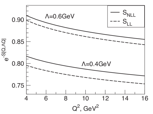
Figure 11: Effect on the FFs from the leading logarithmic summation (LL) for different values of $\Lambda$.

we demonstrate the results for the leading Sudakov logarithm factor $e^{-S(Q,\mu_{h},\mu_{I})}$ taking $\mu_{h}=Q$ and $\mu_{I}=\sqrt{\Lambda Q}$. We use two different values for the soft scale $\Lambda=\{0.4,0.6\}$GeV and consider $Q^{2}=4-16~{}$GeV². For our numerical estimate, we used formula Eq. (99) with the two-loop running coupling[ $N_{f}=4$ and $\alpha_{s}(2~{}$GeV$)=0.31$]. We observe that the Sudakov factor provides a reduction of around $10\%-25\%$ depending on the choice of $\Lambda$, and changes quite slowly in the given range of $Q^{2}$. Therefore we can conclude that the soft spectator scattering contribution may provide quite a substantial effect over an extended range of $Q^{2}$ if  the SCET_I FFs $f_{1,2}$ are not too small.

However, the full next-to-leading evolution includes also single logarithms described by the kernels $U_{A,B}$. In the case of $F_{2}$, the evolution effect from $U_{B}\left[\tau~{};\mu_{h},\mu_{I}\right]$ in Eq. (155) is given by the approximate solution of Eq. (110) and does not depend on the gluon momentum fraction $\tau$. Using Eq. (110) we can write

$$F_{2}^{(s)}(Q) = \frac{m^{2}_{N}}{Q^{2}}e^{-S(Q;\mu_{h},\mu_{I})}\int_{0}^{1}d\tau U_{B}\left[\tau~{};Q,\mu_{I}\right]\ f_{2}(\tau;Q_{I},\mu_{I})$$ (158)

$$\approx \frac{m^{2}_{N}}{Q^{2}}e^{-S(Q;\mu_{h},\mu_{I})}U_{B}^{\text{app}}\left[Q,\mu_{I}\right]\int_{0}^{1}d\tau~{}f_{2}(\tau;Q_{I},\mu_{I}),$$

Therefore in the ratio $F_{2}/F_{1}$ the leading and next-to-leading Sudakov logarithms cancel and we obtain that this quantity depends only on the SCET_I FFs:

$$\frac{Q^{2}F_{2}^{(s)}}{F_{1}^{(s)}}\simeq\frac{U_{B}^{\text{app}}\left[Q,\mu_{I}\right]}{U_{A}\left[Q,\mu_{I}\right]}\frac{m^{2}_{N}\int_{0}^{1}d\tau~{}f_{2}(\tau;Q_{I},\mu_{I})}{~{}f_{1}(Q_{I},\mu_{I})}.$$ (159)

The ratio of the kernels $U_{A,B}$ in Eq. (159) changes slowly, for instance,

$$0.93\leq\frac{U_{B}^{\text{app}}\left[Q,\mu_{I}\right]}{U_{A}\left[Q,\mu_{I}\right]}\leq 0.95\text{ \ \ \ for }4~{}\text{GeV}^{2}\leq Q^{2}\leq 16~{}\text{GeV}^{2}\text{ and }\Lambda=400~{}\text{MeV.}$$ (160)

For large $Q$ values, when $|Q_{I}|\sim\sqrt{\Lambda Q}\rightarrow\infty$ we expect the asymptotic $Q^{2}F_{2}/F_{1}\rightarrow\text{const}$ as it follows from SCET counting rules. It is clear that such asymptotic could be reached only at very large values of $Q^{2}$. Therefore it is not surprising that the ratio, measured recently up to $Q^{2}\lesssim 8.5~{}$GeV² Puckett:2010ac , shows a behavior which drops less fast in $Q^{2}$, when compared with the expected power $Q^{-2}$. For such values of $Q^{2}$ the ratio Eq. (159) is defined practically only by the ratio of the SCET form factors $f_{1,2}$ depending on $Q_{I}$. But the hard-collinear scale in this region is approximately $Q_{I}\sim\sqrt{\Lambda Q}\simeq 0.9-1.3$ GeV, i.e. quite small in order to expect the asymptotic behavior.

We obtained that the effect from the Sudakov suppression in the region of moderate space-like $Q^{2}$ can be estimated as $\sim 10\%-25\%$. However the situation can be different for timelike momenta $q^{2}>0$. In this case, the Sudakov factor after analytical continuation from spacelike to timelike region may produce a substantial enhancement. Properties of the timelike processes have been studied in many publications (see, for instance, Parisi79 ; Magnea90 ; Radyushkin00 ). It is well known that analytic continuation of the Sudakov FF to the timelike region produces enhanced $\pi^{2}$ terms. Such corrections were resummed for different processes Parisi79 ; Magnea90 ; Ahrens08 . In order to perform such resummation it was suggested to perform the matching at a timelike renormalization point $-\mu_{h}^{2}$ Ahrens08 . Then the timelike Sudakov factor $e^{-S_{\text{TL}}}$ accumulates the large $\pi^{2}$ contributions together with the Sudakov logarithms. Using this recipe we must compute $S_{\text{TL}}\equiv S[-q^{2}-i\varepsilon,-\mu_{h}-i\varepsilon,\mu]$ in the timelike region. This can be done with the help of analytical continuation of the running coupling which to our accuracy reads Ahrens08 ; Radyushkin99 :

$$\frac{\alpha_{s}(\mu^{2})}{\alpha_{s}(-\mu^{2})}=1-ia(\mu^{2})+\frac{\beta_{1}}{\beta_{0}}\frac{\alpha_{s}(\mu^{2})}{4\pi}\ln\left[1-ia(\mu^{2})\right]+\mathcal{O}(\alpha_{s}^{2}),$$ (161)

where $a(\mu^{2})=\beta_{0}\alpha_{s}(\mu_{h}^{2})/4$ $\sim\mathcal{O}(1)$ for moderate values of $Q^{2}$.

Existing experimental data for the ratio $R_{M}=|G_{M}(q^{2})|/G_{M}(Q^{2})$ show a considerable enhancement of timelike FFs over their spacelike counterparts: $R_{M}$ $\simeq 1.5-$ $2$ over the range $Q^{2}\sim 10~{}$GeV². Despite that the extraction of the absolute value of the time like FF $|G_{M}(q^{2})|$ involves considerable assumptions about the behavior of the timelike electric FF $G_{E}$ and probably includes large systematic errors, the timelike enhancement is considered as a well established fact. In Ref. Radyushkin00 it was suggested that ”soft terms” accompanied by the Sudakov double logarithms could play an important role in a so-called, $K$-factor type enhancement to hadronic FFs in the timelike region. Using the results of Eqs. (154, 155) with resummed Sudakov logarithms we can easily estimate such an effect in our approach.

In order to study the qualitative effect of the SCET_I evolution we consider the ratio of the Dirac timelike (TL) and spacelike (SL) FFs. Let us introduce:

$$R_{1}=\frac{|F_{1}(q^{2})|}{F_{1}(Q^{2})}\simeq\frac{|e^{-S_{\text{TL}}}|}{e^{-S_{SL}}}\frac{|U_{A}^{\text{TL}}|}{U_{A}}\frac{~{}\left|f_{1}(q_{I},\mu_{I})\right|}{~{}f_{1}(Q_{I},\mu_{I})~{}}.$$ (162)

where we used $q_{I}$ in order to specify timelike momentum transfer $|q_{I}|\sim\sqrt{\Lambda q}$ in the numerator. We assume that the soft spectator scattering mechanism dominates also in timelike kinematics and appropriate quantities are related by analytical continuation. At present we do not know the SCET FFs $f_{1,2}$. However, we can study the pQCD evolution effect  from the resummed logarithms. In Fig.12 we demonstrate the timelike (TL) to spacelike (SL) ratio $|e^{-S_{\text{TL}}}|/e^{-S_{\text{SL}}}$ which represents the Sudakov logarithms in the ratio $R_{1}$.

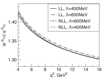
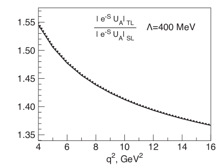
Figure 12: Left panel: Contribution of the timelike (TL) to spacelike (SL) ratio of Sudakov logarithms $|e^{-S_{\text{TL}}}|/e^{-S_{\text{SL}}}$ as function of $q^{2}$ for different choices of $\Lambda$. Solid and dash-dotted curves correspond to LL approximation with $\Lambda=400$ and $600$ MeV respectively; dashed and dotted curves describe next-to-leading approximation. Right panel: complete NLL evolution (including kernel $U_{A}$) with $\Lambda=400$MeV.

One can see that the obtained ratio $|e^{-S_{\text{TL}}}|/e^{-S_{\text{SL}}}$ very weakly depends on the choice of $\Lambda$ and provides an almost $30\%-40\%$ enhancement effect of the timelike FFs relative to their spacelike counterparts. When we combine the Sudakov evolution with the $U_{A}-$kernel of Eq. (100) we obtain the results shown in Fig.12 (right panel). We see that single logarithms increase the ratio by $5\%-8\%$. But this effect is only a small fraction of the full evolution, i.e. non-Sudakov logarithms cannot provide substantial enhancement. Therefore we can conclude that the soft spectator scattering mechanism plays an important role in the discussion of the timelike FF’s. Sudakov logarithms appearing in this case provide an important enhancement in the region of moderate values of timelike momentum transfers $q^{2}$. This enhancement is in qualitative agreement with the extracted absolute value $|G_{M}|$. Moreover, taking account of the simple relation of the pQCD evolution in the spacelike and timelike regions, we can assume that the enhancement in the timelike region suggests an additional, indirect confirmation of the dominance of the soft spectator scattering mechanism in the spacelike region. This might be true if the SCET FFs $f_{1,2}$ are not modified very strongly after analytical continuation from space like to timelike regions.

VI Conclusions

In the present work, we studied the soft rescattering contribution to the nucleon Dirac and Pauli FFs. This work is motivated by phenomenological studies of nucleon FFs suggesting that in the $Q^{2}$ range 5 - 10 GeV², the nucleon FFs are not yet dominated by a hard scattering mechanism involving three active quarks, interacting via hard two-gluon exchange. In the soft rescattering picture studied here, as first suggested by Feynman, the highly virtual photon interacts with one active quark, whereas the other spectator quarks remain soft. Such a picture is characterized by two large scales : the hard scale $Q^{2}$, representing the virtuality of the hard photon probe, and the hard-collinear scale $\Lambda Q$ (with $\Lambda$ a soft scale of order $\sim 0.5$ GeV), corresponding to the virtuality of the active, so-called hard-collinear quark.

By way of example, we started our investigation by calculating within perturbation theory the soft rescattering contributions to the nucleon FFs. Within such perturbative calculation, the three collinear quarks in the initial nucleon wave function are connected to the active hard-collinear quark and two remaining soft quarks through (hard-collinear) two-gluon exchange. Analogously, the hard collinear quark after the interaction with the hard photon also scatters with the remaining two soft quarks through (hard-collinear) two-gluon exchange. For the Dirac FF $F_{1}$, this analysis overlaps with previous work in the literature, whereas for the Pauli FF $F_{2}$ it has been performed for the first time here. We have demonstrated that such a specific two-loop contribution to the nucleon FFs gives the same scaling behavior as the hard region, involving hard two-gluon exchange, i.e., $F_{1}\sim 1/Q^{4}$, and $F_{2}\sim 1/Q^{6}$. Furthermore, the perturbative calculation suggests a factorization formula for the FFs in terms of nucleon distribution amplitudes, describing how the collinear quarks make up the initial and final nucleon, a hard scattering process on the active quark, and a soft correlation function describing the propagation of the remaining two soft spectator quarks.

The specific perturbative calculation demonstrates that a description of the soft rescattering mechanism could be carried out in general in two steps. First, one integrates over hard fluctuations (of order $Q^{2}$), leaving only hard-collinear virtualities (of order $\Lambda Q$) and soft virtualities (of order $\Lambda^{2}$). For large enough scale $Q$, such that $\Lambda Q\gg\Lambda^{2}$, one can then further use perturbation theory and also factorize hard-collinear fluctuations leaving at the end only collinear and soft modes, describing the soft QCD dynamics.

The possibility of such a two-step factorization, with the aim of developing a systematic approach of the soft contribution in the case of nucleon form factors, was addressed for the first time in this paper. A similar approach has also been considered recently for inclusive cross sections in Chay:2010hq . The first step corresponds with the matching of full QCD onto the soft collinear effective field theory at a factorization scale $\mu^{2}_{I}=Q^{2}$, and denoted by SCET_I. Technically, we have demonstrated this step by calculating the leading-order hard coefficient functions in front of the operators constructed from SCET_I fields, corresponding with the Dirac and Pauli FF structures. These leading-order hard coefficient functions involve the emission of hard-collinear transverse gluons, comoving with the active quark. We subsequently resummed the large logarithms of order $\sim\ln Q^{2}/\mu_{I}^{2}$, which appear when evolving the SCET_I operators from the hard scale $Q^{2}$ down to the scale $\mu_{I}^{2}\sim Q\Lambda$. Both for the leading e.m. current operator structure, corresponding with the Dirac FF $F_{1}$, and the subleading operator structure, corresponding with the Pauli FF $F_{2}$, we solved the renormalization group equations for the corresponding coefficient functions, and obtained the NLL solution. This provides a practical check that to NLL accuracy the first-step factorization (so-called SCET_I factorization) for both $F_{1}$ and $F_{2}$ indeed holds.

We next discussed the further matching of the SCET_I theory to the effective theory involving only collinear and soft particles (so-called SCET_II), defined at a factorization scale $\mu^{2}_{II}=Q\Lambda$. As a first step to arrive at such a full factorization formula for the soft rescattering contribution, we analyzed in this work the leading terms in the effective theory. The factorization formula involves two so-called jet functions, describing the amplitude for the transition of three collinear quarks into a hard-collinear (active) quark and two soft quarks; a soft correlation function describing the soft rescattering of the two soft spectator quarks in the background soft-gluon fields emitted by the hard-collinear (active) quark; and the two nucleon distribution amplitudes, describing how the three initial and final collinear quarks make up the nucleons. The jet functions can be computed performing the matching from SCET_I operators onto SCET_II at the factorization scale $\mu_{II}^{2}=Q\Lambda$. Also here large logarithms $\sim\ln\Lambda Q/\mu_{II}^{2}$ arise, when we evolve the factorization scale $\mu_{II}^{2}$ down to value of order $\Lambda^{2}$. They can be resummed again using RG equations. We leave this consideration to a future work.

For the Pauli FF $F_{2}$ we also discussed that an analysis is more involved as there may be a double counting between the hard and soft rescattering mechanisms. Furthermore the matching from SCET_I onto SCET_II does not yield a well defined expression for the Pauli FF, due to end-point singularities, which calls for a more refined treatment for $F_{2}$ in a future publication.

The SCET_I factorization formulas allowed us already to discuss some phenomenological consequences in this work. For the soft rescattering contribution to the $Q^{2}F_{2}/F_{1}$ ratio, we found that the ratio of the next-to-leading order evolution kernels changes only by a few percent in the range $Q^{2}\simeq 4-16$ GeV², and is mainly dominated by SCET_I FFs defined at a corresponding scale $Q^{2}_{I}\sim\Lambda Q\simeq 0.8-1.6$ GeV². Such scale is quite small to expect the asymptotic constant behavior. The experimental data for the $Q^{2}F_{2}/F_{1}$ ratio in this $Q^{2}$ range indeed show rising behavior, in agreement with the above analysis. A second phenomenological consequence of our framework was discussed for the ratio of the spacelike to timelike FF $F_{1}$. We showed that the resummed Sudakov logarithms provide a 30% - 40 % enhancement to this ratio in the range of momentum transfers $q^{2}$ around 10 GeV². This enhancement is in qualitative agreement with the empirical extracted ratio for the absolute value of the dominant FF $G_{M}$ in the timelike as compared to the spacelike region. A more detailed phenomenological analysis requires us to parametrize the SCET_I FFs, which is equivalent to using the SCET_II factorization formula, and express them in terms of DAs, jet functions, and a two-quark soft correlation function, as outlined in this work. Such an analysis remains a challenge for a future work.

Appendix A. Leading order coefficient functions

Here we discuss in detail calculation of leading-order hard coefficient functions. First, Eq. (87) can be rewritten in compact form in momentum space,

$$\bar{q}(0)\gamma^{\mu}q(0)=~{}\text{tr}\left[C^{\mu}(Q,\mu)~{}O^{q}(0)\right]+\int_{0}^{1}d\tau~{}\text{tr}\left[~{}C_{\bar{n}}^{\mu}(\tau,Q,\mu)~{}O_{\bar{n}}^{q}(\tau)+C_{n}^{\mu}(\tau,Q,\mu)~{}O_{n}^{q}(\tau)~{}\right]+~{}...$$ (163)

where we used translation invariance and defined the momentum space coefficients as

$$C^{\mu}(Q,\mu)~{}=\int d\hat{s}_{1}d\hat{s}_{2}~{}\tilde{C}^{\mu}(\hat{s}_{1},\hat{s}_{2})~{}e^{i(P^{\prime}\cdot\bar{n})s_{2}-i(P\cdot n)s_{1}},$$ (164)

$$C_{\bar{n}}^{\mu}(\tau,Q,\mu)~{}=\int d\hat{s}_{1}d\hat{s}_{2}d\hat{s}_{3}~{}e^{-i(P\cdot n)s_{1}}~{}e^{i(P^{\prime}\cdot\bar{n})~{}\tau s_{3}+i(P^{\prime}\cdot\bar{n})~{}\bar{\tau}s_{2}}~{}\tilde{C}_{\bar{n}}^{\mu}(\hat{s}_{1},\hat{s}_{2},\hat{s}_{3}),$$ (165)

$$C_{n}^{\mu}(\tau,Q,\mu)=\int d\hat{s}_{1}d\hat{s}_{2}d\hat{s}_{3}~{}e^{i(P^{\prime}\cdot n)s_{2}}~{}e^{-i(P\cdot n)~{}\tau s_{3}-i(P\cdot n)~{}\bar{\tau}s_{1}}~{}\tilde{C}_{n}^{\mu}(\hat{s}_{1},\hat{s}_{2},\hat{s}_{3}),~{}$$ (166)

Here $P$ and $P^{\prime}$ denote the total hard-collinear momentum of the external state for each jet, and $(P\cdot n)=(P^{\prime}\cdot\bar{n})=Q$ is the large component of each momentum. The variable $\tau$ is the fraction of large momentum component $(P^{\prime}\cdot\bar{n})$ [$(P\cdot n)$] carried by the hard-collinear gluon $\mathcal{A}_{\bot}^{\prime}$ ($\mathcal{A}_{\bot}$), $\bar{\tau}\equiv 1-\tau$. The objects $O_{\bar{n}}^{q}(\tau)$ and $O_{n}^{q}(\tau)$ denote the Fourier transformed SCET operators:

$$O_{\bar{n}}^{q}(\tau)=\int\frac{d\hat{s}_{3}}{2\pi}~{}e^{-is_{3}(P^{\prime}\cdot\bar{n})\tau}~{}\tilde{O}_{\bar{n}}^{q}(0,0,s_{3}),~{}\ \ \ \ O_{n}^{q}(\tau)=\int\frac{d\hat{s}_{3}}{2\pi}~{}e^{is_{3}(P\cdot n)\tau}~{}\tilde{O}_{n}^{q}(0,0,s_{3}).$$ (167)

The tree-level coefficient functions in momentum space  can be obtained from an analysis of the matrix elements in QCD and SCET.  In order to compute $C^{\mu}(Q,\mu)$ defined in Eq. (163) consider the matrix element of the e.m. current between collinear quark states:

$$\left\langle p^{\prime}\left|\bar{q}(0)\gamma^{\mu}q(0)\right|p\right\rangle=\left\langle p^{\prime}\left|\text{tr}\left[C^{\mu}(Q,\mu)~{}O^{q}(0)\right]\right|p\right\rangle.~{}$$ (168)

The subleading term in Eq. (163) does not contribute in this case. Then for the matrix element at LO we obtain:

$$\text{{\it lhs} of Eq.~{}(\ref{C:calc}):~{}\ }\left\langle p^{\prime}\left|\bar{q}(0)\gamma^{\mu}q(0)\right|p\right\rangle_{\text{LO}}=\bar{u}^{\prime}\gamma^{\mu}u=\bar{\xi}^{\prime}\gamma_{\bot}^{\mu}\xi+\mathcal{O}(1/Q),$$ (169)

$$\text{{\it rhs} of Eq.~{}(\ref{C:calc}):}~{}~{}\left\langle p^{\prime}\left|\text{tr}\left[C^{\mu}(Q,\mu)~{}O^{q}(0)\right]\right|p\right\rangle=\text{tr}\left[C^{\mu}(Q,\mu)~{}\bar{\xi}^{\prime}\otimes\xi\right],$$ (170)

where $\xi^{\prime},\xi$ without subscript $hc$ denote large components of Dirac spinors (30) and (31). Comparison (169) and (170) yields

$$C^{\mu}(Q,\mu)=\gamma_{\bot}^{\mu}~{}\delta_{F^{\prime}F}+\mathcal{O}(\alpha_{s}).$$ (171)

where $F^{\prime},F$ describe quark color indices.

In order to compute the subleading coefficient functions one has to consider the matrix element with the quark-gluon external state. We consider an outgoing gluon with hard-collinear momentum $q^{\prime}$ collinear to $p^{\prime}$ and for simplicity we neglect the transverse components of the outgoing momenta. Then we can compute the leading-order contribution to $C_{\bar{n}}^{\mu}(\tau,Q,\mu)$.

We start by considering the QCD calculation. The corresponding diagrams are shown in Fig.13.

Figure 13: QCD tree diagrams required for matching onto the subleading 3-particle operator

For the first graph we have

$$D_{1}=(ig)~{}\bar{u}(p^{\prime})\hbox to0.0pt{\hbox to7.50002pt{\hfil/\hfil}\hss}{A}^{\prime}\frac{i(\hat{p}^{\prime}+\hat{q}^{\prime})}{(p^{\prime}+q^{\prime})^{2}}\gamma^{\mu}u(p) \simeq ~{}(ig)\bar{\xi}^{\prime}\hbox{/}\hbox to0.0pt{\hbox to7.50002pt{\hfil/\hfil}\hss}{A}^{\prime}\left[\frac{\hbox to0.0pt{\hbox to6.00235pt{\hfil/\hfil}\hss}n}{2}\frac{i}{(p^{\prime}+q^{\prime})\cdot n}+\frac{\hbox to0.0pt{\hbox to5.00002pt{\hfil$\bar{n}$\hfil}\hss}/}{2}\frac{i}{(p^{\prime}+q^{\prime})\cdot\bar{n}}\right]\gamma^{\mu}\xi$$ (172)

$$= ~{}(ig)\ \bar{\xi}^{\prime}\left[\hbox to0.0pt{\hbox to7.50002pt{\hfil/\hfil}\hss}{A}_{\bot}^{\prime}\frac{i\bar{n}^{\mu}}{(p^{\prime}+q^{\prime})\cdot\bar{n}}\right]\xi.$$

For clarity, we write $A_{\mu}$ for the external gluon line with momentum $q^{\prime}$ instead of polarization $\varepsilon^{\ast}(q^{\prime})$. The second diagram:

$$D_{2}=(ig)\bar{u}(p^{\prime})\gamma^{\mu}\frac{i(\hat{p}-\hat{q}^{\prime})}{(p-q^{\prime})^{2}}\hbox to0.0pt{\hbox to7.50002pt{\hfil/\hfil}\hss}{A}^{\prime}u(p) \simeq (ig)~{}\bar{\xi}^{\prime}\gamma^{\mu}\left[\frac{\hbox to0.0pt{\hbox to5.00002pt{\hfil$\bar{n}$\hfil}\hss}/}{2}\frac{i}{-(q^{\prime}\cdot\bar{n})}+\frac{\hbox to0.0pt{\hbox to6.00235pt{\hfil/\hfil}\hss}n}{2}\frac{i}{(p\cdot n)}\right]~{}\hbox to0.0pt{\hbox to7.50002pt{\hfil/\hfil}\hss}{A}^{\prime}\xi$$ (173)

$$= ~{}\bar{\xi}^{\prime}\left[~{}(ig)~{}\hbox to0.0pt{\hbox to7.50002pt{\hfil/\hfil}\hss}{A}_{\bot}^{\prime}\frac{in^{\mu}}{(p\cdot n)}\right]\xi.$$

Therefore the sum reads

$$D_{1}+D_{2}=\bar{\xi}^{\prime}\left[~{}(-g)~{}\hbox to0.0pt{\hbox to7.50002pt{\hfil/\hfil}\hss}{A}_{\bot}^{\prime}~{}\left\{\frac{n^{\mu}}{(p\cdot n)}+\frac{\bar{n}^{\mu}}{(p^{\prime}+q^{\prime})\cdot\bar{n}}\right\}\right]\xi,$$ (174)

which involves the transverse gluon field and the longitudinal projection of the e.m. current, as required. It is easy to see that the obtained kinematical structure is e.m. gauge invariant. This term must be compared with the SCET matrix element,

$$~{}\left\langle p^{\prime},q^{\prime}\left|\int_{0}^{1}d\tau~{}\text{tr}\left[~{}C_{\bar{n}}^{\mu}(\tau,Q,\mu)~{}O_{\bar{n}}^{q}(\tau)\right]\right|p\right\rangle=\int_{0}^{1}d\tau~{}~{}\text{tr}~{}[C_{\bar{n}}^{\mu}(\tau,Q,\mu)~{}\left\langle p^{\prime},q^{\prime}\left|~{}O_{\bar{n}}^{q}(\tau)\right|p\right\rangle],$$ (175)

with

$$\left\langle p^{\prime},q^{\prime}\left|~{}O_{\bar{n}}^{q}(\tau)\right|p\right\rangle\simeq\bar{\xi}^{\prime}\hbox to0.0pt{\hbox to7.50002pt{\hfil/\hfil}\hss}{A}_{\bot}^{\prime}\xi~{}~{}\delta\left(\frac{\left(q^{\prime}\cdot\bar{n}\right)}{(p^{\prime}+q^{\prime})\cdot\bar{n}}-~{}\tau\right).$$ (176)

Substituting this into Eq. (175) and comparing this with the QCD result of Eq. (174) we obtain

$$C_{\bar{n}}^{\mu}(\tau,Q,\mu)=-\frac{1}{Q}\left(n^{\mu}+\bar{n}^{\mu}\right)~{}\hat{1}~{}\delta_{F^{\prime}F},$$ (177)

where the symbol $\hat{1}$ denotes the unity operator in Dirac space. Notice that the obtained coefficient function does not depend on the momentum fraction $\tau$ at the LO level. A calculation of the second term with $C_{n}^{\mu}$ can be done in an analogous way. The result can also be obtained without explicit calculations by invoking time reversal invariance which demands the result to be symmetric under $n\leftrightarrow\bar{n}$.

Appendix B. Correspondence between QCD and SCET calculations

In order to illustrate the correspondence of SCET with QCD we here perform the calculation of the jet functions discussed in Sec. II. We start from the calculation of $\mathbf{J}^{\prime}$ defined in (122). In order to have a direct correspondence with the expression (48)

$$J_{(\alpha)}^{\prime}\left[y_{i},\omega_{i}\right]=\frac{1}{Q^{3}}\frac{1}{y_{1}\bar{y}_{3}^{2}}\frac{1}{(\omega_{1}+\omega_{2})^{2}(-\omega_{1})}\left[~{}\bar{\xi}_{3}^{\prime}\right]_{\alpha_{3}}~{}\left[~{}\bar{\xi}_{2}^{\prime}\gamma_{\bot}^{i}\right]_{\alpha_{2}}\left[\bar{\xi}_{1}^{\prime}\gamma_{\bot}^{i}\right]_{\alpha_{1}},$$

we consider the appropriate subprocess

$${\xi}_{hc}(p^{\prime}-k_{1}-k_{2})+q_{s}(k_{1})q_{s}(k_{2})\overset{\text{SCET}_{I}}{\rightarrow}\xi_{c}(y_{1}p^{\prime})~{}\xi_{c}(y_{2}p^{\prime})~{}\xi_{c}(y_{3}p^{\prime}).$$ (178)

described by the matrix element

$$J_{(\alpha)}^{\prime}~{}q_{\alpha_{1}}(k_{1})q_{\alpha_{2}}(k_{2})=\left\langle y_{1}p^{\prime},y_{2}p^{\prime},y_{3}p^{\prime}\right|T\left(\bar{\xi}_{hc}^{\prime}W^{\prime}(0),\mathcal{L}_{\xi q}^{(1)},\mathcal{L}_{\xi q}^{(1)},\mathcal{L}_{\xi}^{(0)}\right)\left|0\right\rangle.$$ (179)

The soft quark fields $q_{s}$ are considered as external. In order to reproduce the expression in Eq. (48) we need the diagram shown in Fig.14.

Figure 14: One of the diagrams describing subprocess (178) in SCET_I. The soft fields are considered as external fields, and outgoing quarks are collinear.

From the Lagrangians $\mathcal{L}_{\xi}^{(0)}$ and $\mathcal{L}_{q\xi}^{(1)}$ one can easily define the Feynman rules. They were already presented in the literature (see, e.g., Refs. Bauer2000 ; Pirjol2002 ; Beneke:2005gs ). For the convenience of the reader we reproduce the relevant vertices here. Taking account of only the required leading-order terms one obtains

$$\begin{tabular}[c]{l}{\includegraphics[natheight=0.583800in,natwidth=0.947800in,height=42.19131pt,width=68.49748pt]{SCET-soft-collinear-vertex-1.pdf}}\end{tabular}\ \simeq ig\left[T^{a}\right]_{AB}\left[\gamma_{\bot}^{\mu}\right]_{\alpha\beta}~{},~{}\ \begin{tabular}[c]{l}{\includegraphics[natheight=0.499000in,natwidth=0.837100in,height=36.06221pt,width=60.49701pt]{SCET-hc-hc-c-vertex.pdf}}\end{tabular}\ \simeq ig\left[T^{a}\right]_{AB}\frac{\hbox to0.0pt{\hbox to5.00002pt{\hfil$\bar{n}$\hfil}\hss}/}{2}n^{\mu}.$$ (180)

$$\begin{tabular}[c]{l}{\includegraphics[natheight=0.667600in,natwidth=1.017900in,height=48.24763pt,width=73.56352pt]{SCET-xiAAq-vertex-2g.pdf}}\end{tabular}\ \simeq-ig^{2}\left(\left[T^{a}T^{b}\right]_{AB}\left[\gamma_{\bot}^{\mu}\right]_{\alpha\beta}\frac{\bar{n}^{\nu}}{(q_{2}\cdot\bar{n})}+\left[T^{a}T^{b}\right]_{AB}\left[\gamma_{\bot}^{\nu}\right]_{\alpha\beta}\frac{\bar{n}^{\mu}}{(q_{1}\cdot\bar{n})}\right)~{}.$$ (181)

Assuming the same choice of momenta as in Fig. 3, we obtain the following analytical expression

$$J_{(\alpha)}^{\prime}q_{\alpha_{1}}(k_{1})q_{\alpha_{2}}(k_{2}) \sim \bar{\xi}_{1}^{\prime}\gamma_{\bot}^{\nu}T^{b}q(k_{1})\bar{\xi}_{2}^{\prime}\left\{-\frac{\bar{n}^{\mu}\gamma_{\bot}^{\nu}}{\left(p_{4g}\cdot\bar{n}\right)}T^{b}T^{a}\right\}q(k_{2})\bar{\xi}_{3}^{\prime}\frac{\hbox to0.0pt{\hbox to5.00002pt{\hfil$\bar{n}$\hfil}\hss}/\hbox to0.0pt{\hbox to6.00235pt{\hfil/\hfil}\hss}n}{4}\left\{T^{a}n^{\mu}\right\}\frac{1}{(p_{3g}\cdot n)}\frac{1}{p_{3g}^{2}}\frac{1}{p_{4g}^{2}}$$ (182)

$$\sim \frac{1}{(k_{1}^{+}+k_{2}^{+})^{2}}~{}\frac{1}{\left(-~{}k_{1}^{+}\right)}~{}\frac{1}{Q^{3}}\frac{1}{y_{1}\bar{y}_{3}^{2}}~{}\bar{\xi}_{1}^{\prime}\gamma_{\bot}^{i}q(k_{1})~{}\bar{\xi}_{2}^{\prime}\gamma_{\bot}^{i}q(k_{2})~{}[\bar{\xi}_{3}^{\prime}]_{\alpha_{3}}$$

$$= \int d\omega_{1,2}~{}J_{(\alpha)}^{\prime}\left[y_{i},\omega_{i}\right]~{}~{}q_{\alpha_{1}}(k_{1})~{}q_{\alpha_{2}}(k_{2})~{}\delta(\omega_{1}-k_{1}^{+})\delta(\omega_{2}-k_{2}^{+}).$$

with the same $J_{(\alpha)}^{\prime}$ as in Eq. (48). Consider the color structure which we ignored in the calculation in Sec. II. Projecting the color indices of the outgoing collinear quarks onto the colorless nucleon, we obtain :

$$\frac{\varepsilon^{i^{\prime}j^{\prime}k^{\prime}}}{3!}\left[T^{b}\right]_{i^{\prime}i}\otimes\left[T^{b}T^{a}\right]_{j^{\prime}j}\otimes\left[T^{a}\right]_{k^{\prime}k}=\frac{2}{27}\varepsilon^{ijk}.$$ (183)

The resulting antisymmetrical tensor $\varepsilon^{ijk}$ is then contracted with the color indices of the soft fields yielding the soft operator in Eq. (131).

Consider now the helicity flip FF $F_{2}$. Again, from the QCD calculation we obtained the result of Eq. (II.2):

$$J_{(\alpha)}^{\prime}\left[y_{i},\omega_{i}\right]=\frac{1}{Q^{2}}\frac{\left[\bar{\xi}_{1}^{\prime}\gamma_{\bot}^{\alpha}\right]_{\alpha_{1}}\left[\bar{\xi}_{2}^{\prime}\gamma_{\bot}^{\alpha}\right]_{\alpha_{2}}~{}\left[\bar{\eta}_{3}^{\prime}~{}\hat{n}\right]_{\alpha_{3}}}{~{}\bar{y}_{1}y_{3}(\omega_{2}+\omega_{3})\omega_{3}^{2}},$$ (184)

In this case, we have to consider the presence of the small component $\bar{\eta}_{3}^{\prime}$. In SCET this field is eliminated by the equation of motion, yielding

$$\bar{\eta}_{c}^{\prime}\simeq-~{}\bar{\xi}^{\prime}i\hat{D}_{\bot c}\frac{\hbox to0.0pt{\hbox to5.00002pt{\hfil$\bar{n}$\hfil}\hss}/}{2}(i\bar{n}\cdot\overleftarrow{D}_{c})^{-1}.$$ (185)

In order to have a connection with the QCD result of Eq. (II.2), we must substitute

$$\bar{\eta}_{c}^{\prime}=\bar{\xi}_{c}^{\prime}i\hat{D}_{\bot c}(i\bar{n}\overleftarrow{D}_{c})^{-1}\frac{\hbox to0.0pt{\hbox to5.00002pt{\hfil$\bar{n}$\hfil}\hss}/}{2}\simeq\bar{\xi}_{c}^{\prime}\hat{A}_{c\bot}(i\bar{n}\cdot\overleftarrow{\partial})^{-1}\frac{\hbox to0.0pt{\hbox to5.00002pt{\hfil$\bar{n}$\hfil}\hss}/}{2}.$$ (186)

From this expression one can see that such a state consists of a collinear quark and a transverse gluon, as is shown in Fig. 9. The corresponding vertex is generated by the Lagrangian $\mathcal{L}_{\xi q}^{(1)}$, includes 2 gluons, and can be associated with the following combination:

$$\bar{\xi}_{hc}~{}i\hat{D}_{\bot}Wq \simeq \bar{\xi}_{c}~{}g\hbox to0.0pt{\hbox to7.50002pt{\hfil/\hfil}\hss}A_{\bot c}^{\prime}~{}\left[\frac{i}{\left(\bar{n}\partial\right)}~{}ig\bar{n}\cdot A_{hc}\right]q=~{}\bar{\xi}_{c}^{\prime}~{}g\hbox to0.0pt{\hbox to7.50002pt{\hfil/\hfil}\hss}A_{\bot c}^{\prime}(\bar{n}\cdot\overleftarrow{\partial})^{-1}\frac{\hbox to0.0pt{\hbox to5.00002pt{\hfil$\bar{n}$\hfil}\hss}/}{2}~{}g\hat{A}_{hc}\frac{\hbox to0.0pt{\hbox to5.00002pt{\hfil$\bar{n}$\hfil}\hss}/\hbox to0.0pt{\hbox to6.00235pt{\hfil/\hfil}\hss}n}{4}q(k_{3})$$ (187)

$$= \left[\bar{\eta}_{c}^{\prime}\hbox to0.0pt{\hbox to7.50002pt{\hfil/\hfil}\hss}A_{\bot c}^{\prime}(\bar{n}\cdot\overleftarrow{\partial})^{-1}\frac{\hbox to0.0pt{\hbox to5.00002pt{\hfil$\bar{n}$\hfil}\hss}/}{2}\right]~{}\hat{A}_{hc}\frac{\hbox to0.0pt{\hbox to5.00002pt{\hfil$\bar{n}$\hfil}\hss}/\hbox to0.0pt{\hbox to6.00235pt{\hfil/\hfil}\hss}n}{4}~{}q(k_{3}).$$

Therefore, we obtain for the diagram in Fig.14 (again ignoring color structures) :

$$J_{(\alpha)}^{\prime}~{}q_{\alpha_{2}}(k_{2})q_{\alpha_{3}}(k_{3}) \sim \left[\bar{\xi}_{1}^{\prime}\gamma_{\bot}^{\mu}\right]_{\alpha_{1}}\bar{\xi}_{2}^{\prime}\left\{n^{\nu}\right\}\frac{\hbox to0.0pt{\hbox to5.00002pt{\hfil$\bar{n}$\hfil}\hss}/\hbox to0.0pt{\hbox to6.00235pt{\hfil/\hfil}\hss}n}{4}\frac{1}{k_{3}^{+}}\gamma_{\bot}^{\mu}q(k_{2})~{}\bar{\eta}_{3}^{\prime}\gamma^{\nu}\frac{\hbox to0.0pt{\hbox to5.00002pt{\hfil$\bar{n}$\hfil}\hss}/\hbox to0.0pt{\hbox to6.00235pt{\hfil/\hfil}\hss}n}{4}q(k_{3})~{}\frac{1}{y_{3}Qk_{3}^{+}}\frac{1}{\bar{y}_{1}Q(k_{2}^{+}+k_{3}^{+})}$$ (188)

$$\sim \frac{1}{Q^{2}}\frac{\left[\bar{\xi}_{1}^{\prime}\gamma_{\bot}^{\alpha}\right]_{\alpha_{1}}\left[\bar{\xi}_{2}^{\prime}\gamma_{\bot}^{\alpha}\right]_{\alpha_{2}}~{}\left[\bar{\eta}_{3}^{\prime}~{}\hat{n}\right]_{\alpha_{3}}}{\bar{y}_{1}y_{3}~{}(k_{2}^{+}+k_{3}^{+})\left(k_{3}^{+}\right)^{2}}q_{\alpha_{2}}(k_{2})~{}q_{\alpha_{3}}(k_{3})$$

$$= \int d\omega_{1,2}~{}J_{\mathbf{\alpha}}^{\prime}\left[y_{i},\omega_{i}\right]~{}~{}q_{\alpha_{1}}(k_{1})~{}q_{\alpha_{2}}(k_{2})~{}\delta(\omega_{1}-k_{1}^{+})\delta(\omega_{2}-k_{2}^{+}),$$

with the same $J_{(\alpha)}^{\prime}$  as in Eq. (184).

Using these two examples, we demonstrated that the SCET correctly reproduces the tree-level hard-collinear subprocesses computed before in QCD.

References

- (1) C. E. Hyde-Wright and K. de Jager, Ann. Rev. Nucl. Part. Sci. 54, 217 (2004).
- (2) J. Arrington, C. D. Roberts and J. M. Zanotti, J. Phys. G 34, S23 (2007).
- (3) C. F. Perdrisat, V. Punjabi and M. Vanderhaeghen, Prog. Part. Nucl. Phys. 59, 694 (2007).
- (4) M. K. Jones et al. [Jefferson Lab Hall A Collaboration], Phys. Rev. Lett. 84, 1398 (2000).
- (5) V. Punjabi et al., Phys. Rev. C 71, 055202 (2005) [Erratum-ibid. C 71:069902 (2005)].
- (6) O. Gayou et al. [Jefferson Lab Hall A Collaboration], Phys. Rev. Lett. 88, 092301 (2002).
- (7) A. J. R. Puckett et al., Phys. Rev. Lett. 104, 242301 (2010).
- (8) M. Sudol et al., Eur. Phys. J. A 44, 373 (2010).
- (9) V. L. Chernyak and A. R. Zhitnitsky, Phys. Rept. 112, 173 (1984).
- (10) G. P. Lepage and S. J. Brodsky, Phys. Lett. B 87, 359 (1979).
- (11) A. Duncan and A. H. Mueller, Phys. Rev. D 21, 1636 (1980).
- (12) A. I. Milshtein and V. S. Fadin, Yad. Fiz. 33, 1391 (1981).
- (13) A. I. Milshtein and V. S. Fadin, Yad. Fiz. 35, 1603 (1982).
- (14) V. V. Sudakov, Sov. Phys. JETP 3, 65 (1956) [Zh. Eksp. Teor. Fiz. 30, 87 (1956)].
- (15) J. Bolz, R. Jakob, P. Kroll, M. Bergmann and N. G. Stefanis, Z. Phys. C 66, 267 (1995).
- (16) R. P. Feynman, “Photon-Hadron Interactions,” Reading, 1972, 282p.
- (17) N. Isgur and C. H. Llewellyn Smith, Phys. Rev. Lett. 52, 1080 (1984).
- (18) N. Isgur and C. H. Llewellyn Smith, Nucl. Phys. B 317, 526 (1989).
- (19) N. Isgur and C. H. Llewellyn Smith, Phys. Lett. B 217, 535 (1989).
- (20) B. L. Ioffe and A. V. Smilga, Nucl. Phys. B 216, 373 (1983).
- (21) V. A. Nesterenko and A. V. Radyushkin, Phys. Lett. B 115, 410 (1982).
- (22) V. M. Braun, A. Lenz, N. Mahnke and E. Stein, Phys. Rev. D 65, 074011 (2002).
- (23) V. M. Braun, A. Lenz and M. Wittmann, Phys. Rev. D 73, 094019 (2006).
- (24) A. P. Bakulev, A. V. Radyushkin and N. G. Stefanis, Phys. Rev. D 62, 113001 (2000).
- (25) V. Braun, R. J. Fries, N. Mahnke and E. Stein, Nucl. Phys. B 589, 381 (2000) [Erratum-ibid. B 607, 433 (2001)] .
- (26) C. W. Bauer, S. Fleming and M. E. Luke, Phys. Rev. D 63, 014006 (2000).
- (27) C. W. Bauer, S. Fleming, D. Pirjol and I. W. Stewart, Phys. Rev. D 63, 114020 (2001).
- (28) C. W. Bauer and I. W. Stewart, Phys. Lett. B 516, 134 (2001).
- (29) C. W. Bauer, D. Pirjol and I. W. Stewart, Phys. Rev. D 65, 054022 (2002).
- (30) M. Beneke, A. P. Chapovsky, M. Diehl and T. Feldmann, Nucl. Phys. B 643, 431 (2002).
- (31) M. Beneke and T. Feldmann, Phys. Lett. B 553, 267 (2003).
- (32) M. Beneke and T. Feldmann, Nucl. Phys. B 685, 249 (2004).
- (33) R. J. Hill and M. Neubert, Nucl. Phys. B 657, 229 (2003).
- (34) T. Becher, R. J. Hill, M. Neubert, Phys. Rev. D69 (2004) 054017. [hep-ph/0308122].
- (35) M. Beneke, T. Feldmann, Nucl. Phys. B685 (2004) 249-296. [hep-ph/0311335].
- (36) C. W. Bauer, M. P. Dorsten, M. P. Salem, Phys. Rev. D69 (2004) 114011. [hep-ph/0312302].
- (37) A. V. Manohar, Phys. Lett. B633 (2006) 729-733. [hep-ph/0512173].
- (38) A. V. Manohar, Phys. Rev. D 68, 114019 (2003).
- (39) T. Becher, M. Neubert and G. Xu, JHEP 0807, 030 (2008).
- (40) J. Chay and C. Kim, Phys. Rev. D 65, 114016 (2002).
- (41) D. Pirjol and I. W. Stewart, Phys. Rev. D 67, 094005 (2003) [Erratum-ibid. D 69, 019903 (2004)].
- (42) C. W. Bauer, D. Pirjol and I. W. Stewart, Phys. Rev. D 68, 034021 (2003).
- (43) M. Beneke, Y. Kiyo and D. s. Yang, Nucl. Phys. B 692, 232 (2004).
- (44) R. J. Hill, T. Becher, S. J. Lee and M. Neubert, JHEP 0407, 081 (2004).
- (45) J. Chay and C. Kim, Phys. Rev. D 75, 016003 (2007).
- (46) G. P. Korchemsky and A. V. Radyushkin, Nucl. Phys. B 283, 342 (1987).
- (47) M. Beneke and D. Yang, Nucl. Phys. B 736, 34 (2006).
- (48) C. W. Bauer, D. Pirjol and I. W. Stewart, Phys. Rev. D 67, 071502 (2003).
- (49) C. W. Bauer, D. Pirjol and I. W. Stewart, Phys. Rev. D 68, 034021 (2003).
- (50) N. Kivel, M. Vanderhaeghen, in preparation.
- (51) V. M. Braun, S. E. Derkachov, G. P. Korchemsky and A. N. Manashov, Nucl. Phys. B 553, 355 (1999).
- (52) A. V. Belitsky, X. d. Ji and F. Yuan, Phys. Rev. Lett. 91, 092003 (2003).
- (53) G. Parisi, Phys. Lett. B 90, 295 (1980).
- (54) L. Magnea and G. F. Sterman, Phys. Rev. D 42, 4222 (1990).
- (55) V. Ahrens, T. Becher, M. Neubert and L. L. Yang, Phys. Rev. D 79, 033013 (2009).
- (56) A. V. Radyushkin, JINR Rapid Commun. 78, 96 (1996).
- (57) J. Chay and C. Kim, arXiv:1007.4395 [hep-ph].