Absolute Measure of Local Chirality and the Chiral Polarization Scale of the QCD Vacuum

Abstract:

The use of the absolute measure of local chirality is championed since it has a uniform distribution for randomly reshuffled chiral components so that any deviations from uniformity in the associated ”X-distribution” are directly attributable to QCD-induced dynamics. We observe a transition in the qualitative behavior of this absolute X-distribution of low-lying eigenmodes which, we propose, defines a chiral polarization scale of the QCD vacuum.

1 Introduction

Important properties of the QCD vacuum can be studied indirectly by looking at the characteristics of individual low-lying overlap fermion eigenmodes, which provide a natural way to filter out UV fluctuations. The space-time chiral structure of the eigenmodes reflects the space-time topological structure of the underlying gauge fields. Properties of the “$X$–distribution”[1], the probability distribution of the local chiral-orientation parameter, stirred a debate [2] whether this offered evidence in favor of, or against, models of the QCD vacuum. We revisited [3, 4] the use of the local chiral-orientation parameter and found that most of the qualitative features of the distribution were a kinematical effect which was removed with the use of an improved and absolute measure of local chirality. Here we flesh out the construction of the “absolute $X$–distribution” and proceed to analyze the striking change in its behavior as the energy scale of the eigenmodes is scanned [4].

2 Local Chirality and the $X$–Distribution

The local-chirality parameter measures the tendency of a low-lying Dirac eigenmode, $\psi=\psi_{L}+\psi_{R}$ to be left or right handed. Sampling the space-time values of a particular set of eigenmodes, say at a particular energy scale, for a set of configurations yields (a statistical approximation of) a base probability distribution ${\cal P}_{b}(q_{1},q_{2})$ where $q_{1}\equiv|\psi_{L}|$ and $q_{2}\equiv|\psi_{R}|$. A scatter plot of such a distribution for a particular set of modes is shown in the left panel of Figure 1. We can elucidate the tendency for polarization by integrating over the radial coordinate, $\rho$, and investigating the dependence on the polar angle, $\varphi$.

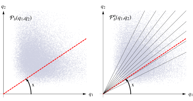
Figure 1: Left: Dynamics governing the polarization properties of two lowest modes for ensemble $E_{1}$ (defined in Table 1). Right: The associated “uncorrelated” dynamics; solid gray lines separate the quadrant into 10 sectors, each containing 10% of the population describing ${{\cal P}}_{b}^{u}$.

It is convenient to symmetrize the angular variable $\varphi\in[0,\pi/2]$ by defining the “reference polarization coordinate” $x\equiv\frac{4}{\pi}\varphi-1$ so that $x\in[-1,+1]$ and such that a value of $x=+1$ ($x=-1$) corresponds to purely right handed (left handed) bispinors [1]. Thus, in the literature [2], histograms which have a “double-peak,” that is two peaks near $x=\pm 1$ in a distribution symmetric about $x=0$, have been interpreted (prematurely as we will see) as revealing that the eigenmodes display chiral polarization. The amount of peaking can be enhanced with a different choice of “polarization function,” that is, using functions of $x$, rather than $x$ itself. These polarization functions can be classified as belonging to one of several families, such as

$${\mathscr{X}}^{C}(x;\alpha)=\mathop{\rm sgn}(x)\;|x|^{\alpha}\quad;\quad{\mathscr{X}}^{R}(t;\alpha)=\frac{t^{\alpha}-1}{t^{\alpha}+1}\quad;\quad{\mathscr{X}}^{G}(t;\alpha)=\frac{4}{\pi}\tan^{-1}(t^{\alpha})-1$$ (1)

where $\alpha>0$ and $t\equiv\tan(\varphi)$. ${\mathscr{X}}^{C}(x;1)=x={\mathscr{X}}^{G}(t;1)$ correspond to the original chiral orientation parameter [1]. ${\mathscr{X}}^{G}(t;2)$ and ${\mathscr{X}}^{R}(t;2)$ are alternatives that appeared in the literature [2]. All of these choices of polarization functions share the same crucial features of the simplest choice of the reference polarization function ${\mathscr{X}}(x)=x$, namely they are odd, monotonically-increasing functions.

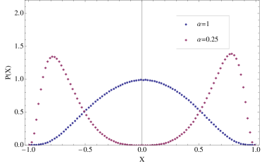
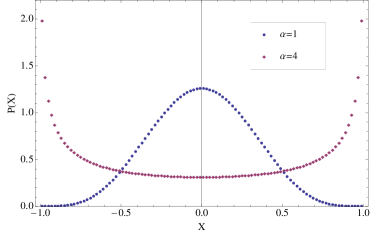
Figure 2: Possible $X$–distributions associated with fixed dynamics can have qualitatively different behavior. Here we select two polarization functions from family ${\mathscr{X}}^{C}$ (left), and two from family ${\mathscr{X}}^{R}$ (right). In this and subsequent figures, the data have error bars but they may to be too small to be resolved.

The marginal distribution

$$P(X) = \int_{0}^{\infty}dq_{1}\int_{0}^{\infty}dq_{2}\,{{\cal P}}_{b}(q_{1},q_{2})\;\delta\Bigl{(}X-{\mathscr{X}}(q_{1},q_{2})\Bigr{)}$$ (2)

where $X$ is a generic independent variable parametrizing the range of polarization functions, i.e. $X\in[-1,+1]$, is called the “$X$–distribution” [1]. It depends not only on the dynamical base probability ${\cal P}_{b}(q_{1},q_{2})$ but also on the polarization function ${\mathscr{X}}(x)$ used to measure it. As Fig. 2 indicates, the qualitative features of the $X$–distributions depend very strongly on the choice of the polarization function, and one might be led into declaring, perhaps falsely, that the distribution is highly polarized or highly unpolarized depending on ones arbitrary choice.

Indeed, most of the qualitative appearance of an $X$–distribution is a result of ”kinematics” (or ”phase space”) and is not due to QCD correlations at all [3]. To demonstrate this, we compute the $X$–distribution arising from $\psi_{L}(y)$ and $\psi_{R}(y)$, where $y$ is the spacetime coordinate, and then randomly reshuffle the fields $\psi_{Lran}(y)\equiv\psi_{L}(y_{ran})$, where $y_{ran}$ is a random permutation, using an independent random reshuffle for $\psi_{R}(y)$. Any QCD-dynamically-induced correlation between $\psi_{L}(y)$ and $\psi_{R}(y)$ at site $y$ is destroyed by this procedure. Nevertheless, the correlated and uncorrelated scatter plots of the base probability distributions are very similar as is seen in Fig. 1. Accordingly, when we re-compute the $X$–distribution, the randomized uncorrelated $X$–distribution looks very similar to the original as seen in Fig. 3.

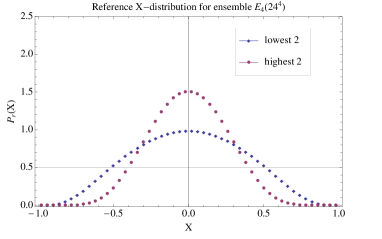
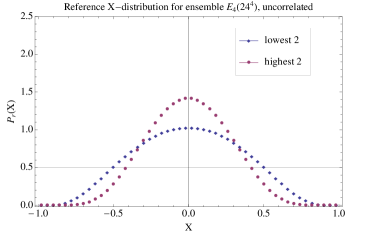
Figure 3: The reference $X$–distribution for “lowest” and “highest” modes in ensemble $E_{4}$ (defined in Table 1) is shown in the left panel. The associated distribution with statistically independent left–right components (“uncorrelated”) is shown in the right panel.

3 The Absolute $X$–Distribution

To expose the true correlation we need to ”subtract” the phase space background, or more precisely measure the (QCD-dynamically-generated) correlated distribution relative to the (randomized) uncorrelated one.

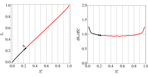
Figure 4: Steps in the construction of absolute $X$–distribution for data shown in Fig. 1. See the discussion in the text.

The following procedure makes a differential comparison of polarization in the dynamics ${\cal P}_{b}(q_{1},q_{2})$ to that of uncorrelated probability distribution ${\cal P}_{b}^{u}(q_{1},q_{2})\equiv p(q_{1})p(q_{2})$, where $p(q_{1})=\int_{-1}^{+1}dq_{2}{\cal P}_{b}(q_{1},q_{2})$ is a marginal distribution: A ray that passes through the origin is specified by its reference polarization coordinate $x$, as shown in Fig. 1. Determine the fraction of population contained between the $q_{1}$-axis and this ray, separately for ${\cal P}_{b}(q_{1},q_{2})$ and for ${\cal P}_{b}^{u}(q_{1},q_{2})$. These fractions are the cumulative probability functions $S_{r}(x)=\int_{-1}^{x}dx^{\prime}P(x^{\prime})$ and $S_{r}^{u}(x)=\int_{-1}^{x}dx^{\prime}P_{u}(x^{\prime})$. Eliminating $x$, every ray is represented by a point in the cumulative distribution plane $(S_{r}^{u},S_{r})$ with the set of all such points forming a curve starting at $(0,0)$ and ending at $(1,1)$. If the the two dynamics in question have identical polarizations the graph will be a straight line. On the left side of Fig. 4 we plot the result of this construction for data displayed in Fig. 1. The correlated and uncorrelated dynamics have very similar polarizations since the graph is close to being linear. To obtain a differential comparison, and to better see the differences, we compute the slope of the cumulative polarization graph and show it on the right side of Fig. 4. As one can clearly see now, the correlated dynamics exhibits a small excess of polarization with respect to the uncorrelated one near the extremal values. This is a plot of the “absolute $X$–distribution”

$$P_{A}=\frac{1}{2}\frac{dS_{r}}{dS_{r}^{u}}$$ (3)

except for the additional rescaling $S_{r}^{u}\rightarrow X\equiv 2S_{r}^{u}-1$ required since $X\in[-1,+1]$ while the uncorrelated cumulative probability $S_{r}^{u}\in[0,+1]$. This construction is manifestly independent of the choice for polarization coordinate, with different possibilities corresponding to different parametric representations of the same curve in the $(S_{r}^{u},S_{r})$ plane.

Fig. 5 shows the absolute $X$–distribution $P_{A}(X)$ for the lowest two non-zero pairs (left panel) and the highest two (of those measured) from ensemble $E_{5}$ (defined in Table 1). In comparison is shown the uncorrelated $X$–distribution, $P_{r}^{u}(x)$, constructed using the reference polarization coordinate $x$. The shape of $P_{A}(X)$ is determined by the correlation induced by QCD dynamics, while the shape of $P_{r}^{u}(x)$ is determined completely by the kinematics. From the pair, $P_{A}(X)$ and $P_{r}^{u}(x)$, one could reconstruct the correlated (and uncorrelated) $X$–distributions for any choice of polarization function ${\mathscr{X}}(x)$, such as those chosen in [2].

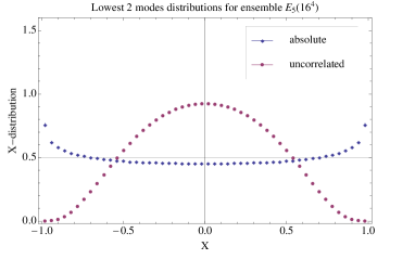
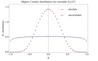
Figure 5: Absolute (dynamical) and uncorrelated (kinematical) $X$–distributions for gauge ensemble $E_{5}$ (defined in Table 1) using the reference polarization coordinate for the latter. Results for lowest two non–zero pairs are shown on the left while the highest two pairs are shown on the right.

4 Convexity or Concavity of Absolute $X$–Distributions

Now we look at the $X$–distributions for the lowest and highest modes (of those measured low-lying modes) for our finest ($24^{4}$) ensemble ($E_{4}$). We have a total of four ensembles on lattices at various lattice spacings, with fixed volume, and a fifth to check for finite-size effects. These are listed in Table 1.

Ensemble	Size	$N_{\rm config}$	Volume	Lattice Spacing	$\Lambda_{\rm LOW}^{\rm MAX}$	$\Lambda_{\rm LOW}^{\rm AVE}$	$\Lambda_{\rm HIGH}^{\rm MIN}$	$\Lambda_{\rm HIGH}^{\rm AVE}$
$E_{1}$	$8^{4}$	100	$(1.32\mathop{\rm fm})^{4}$	$0.165\mathop{\rm fm}$	449	226	1956	1980
$E_{2}$	$12^{4}$	97	$(1.32\mathop{\rm fm})^{4}$	$0.110\mathop{\rm fm}$	407	169	1711	1735
$E_{3}$	$16^{4}$	99	$(1.32\mathop{\rm fm})^{4}$	$0.0825\mathop{\rm fm}$	304	142	1513	1553
$E_{4}$	$24^{4}$	96	$(1.32\mathop{\rm fm})^{4}$	$0.055\mathop{\rm fm}$	344	136	1338	1366
$E_{5}$	$16^{4}$	99	$(1.76\mathop{\rm fm})^{4}$	$0.110\mathop{\rm fm}$	162	58	1087	1123

Table 1: The summary of five ensembles used in overlap eigenmode calculations. The right side of the table describes some properties of the spectra (in MeV) with $\Lambda_{\rm LOW}^{\rm AVE}$ denoting the average magnitude of lowest near–zero eigenvalue over the ensemble and $\Lambda_{\rm HIGH}^{\rm AVE}$ denoting the same for highest eigenvalue. $\Lambda_{\rm LOW}^{\rm MAX}$ is the magnitude of the maximal lowest eigenvalue, and $\Lambda_{\rm HIGH}^{\rm MIN}$ the magnitude of the minimal highest eigenvalue.

Figure 3 (left panel) shows the (reference) $X$–distribution for the lowest pair of eigenmodes and for the highest pair (of the 55 measured). “Subtracting” from this the corresponding $X$–distribution for randomized data leaves the absolute $X$–distribution, $P_{A}(X)$, shown Fig. 6. We see that much of the peaking in the reference $X$–distribution has been removed, by the comparison to the uncorrelated version. This indicates that most of the peaking was kinematical rather than dynamical in the original reference distribution and that to draw any conclusions from this distribution would be misleading at best. On the other hand, for the absolute $X$–distribution, any deviations from uniformity are attributable to correlations induced by QCD dynamics. There is a relatively small but clear effect exhibited by the lowest modes which have a convex shape and the higher modes which have a concave $X$–distribution. That is to say, the lowest modes exhibit an enhanced chiral polarization while the higher modes exhibit a suppression, which we regard as a novel and tantalizing discovery.

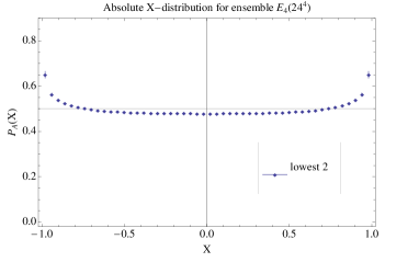
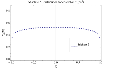
Figure 6: A plot of the absolute $X$–distribution for the “lowest” (left panel) and “highest” (right panel) modes for our finest ensemble.

5 Chiral Polarization Scale

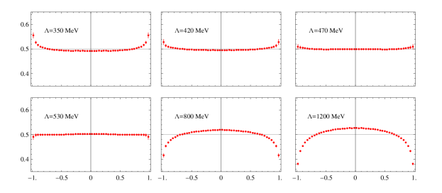
Figure 7: Absolute $X$–distributions for gauge ensemble $E_{4}$ with changing scale $\Lambda$ of the modes. Note the transition from convex to concave (positive to negative correlation) between 470 MeV and 530 MeV.

From Figs. 6 and 7 we see that the shape of the absolute $X$–distribution curve is qualitatively different for the lowest several modes (convex) versus higher modes (concave). We seek the scale $\Lambda_{T}$ at which the transition from convex to concave occurs. To do this we first define, as a figure of merit, a dynamical correlation coefficient in terms of the first moment of the absolute $X$–distribution.

$$C_{A}(X)=-1+2\int^{1}_{-1}dX|X|P_{A}(X)$$

for which $C_{A}>0$ for enhanced polarization, $C_{A}<0$ for suppressed polarization, and $C_{A}=0$ for neutrality as for the case of statistical independence.

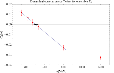
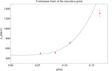
Figure 8: Left panel: Determination of the chiral polarization scale, $\Lambda_{T}$, for the finest lattice. Right panel: Dependence of the chiral polarization scale, $\Lambda_{T}(V,a)$ on the lattice spacing at finite volume.

Fig. 8 (left panel) shows that the dynamical correlation coefficient decreases monotonically from positive values at low modes to negative values at higher modes. A linear interpolation determines the scale $\Lambda_{T}$, at which it crosses zero, at which point there is no dynamical tendency for enhancement or suppression of local chirality in comparison to the associated $X$–distribution for randomized, uncorrelated left-right components.

We repeated the determination of this scale for each of four lattice spacings in order to look for a continuum limit. Fig. 8 (right panel) suggests that $\Lambda_{T}(V,a)$ has a finite continuum limit at fixed volume. A fit to the form $c_{1}+c_{2}a^{4}$, with the coarsest lattice excluded from the fit, is drawn to guide the eye. Further studies must address whether this “chiral polarization scale” survives in the infinite-volume limit, but our check of the finite volume effect at a single lattice spacing is encouraging.

6 Summary

$X$–distributions are detailed probes of QCD dynamics. The use of previous definitions in the literature is misleading, since the distributions are dominated by kinematical effects. It is imperative to use the absolute $X$–distribution as it removes kinematical effects leaving correlations induced by QCD dynamics. We have discovered that the absolute $X$–distributions of the lowest several Dirac eigenmodes are convex (polarized) and those of higher modes are concave (anti-polarized). We have determined the scale $\Lambda_{T}$ of the transition; its continuum limit is finite (at least for finite volume) and, it is proposed, can define a ”chiral polarization” scale of QCD. Complete details are in reference [4]. The absolute $X$–distribution was first discussed in [3].

References

- [1] I. Horv th et al., Phys. Rev. D65 (2002) 014502.
- [2] T. DeGrand, A. Hasenfratz, Phys. Rev. D65 (2002) 014503; R.G. Edwards, U.M. Heller, Phys. Rev. D65 (2002) 014505; I. Hip et al., Phys. Rev. D65 (2002) 014506; T. Blum et al., Phys. Rev. D65 (2002) 014504; C. Gattringer et al., Nucl. Phys. B618 (2001) 205; N. Cundy, M. Teper, U. Wenger, Phys. Rev. D66 (2002) 094505; C. Gattringer, Phys. Rev. Lett. 88 (2002) 22160; P. Hasenfratz et al., Nucl. Phys. B643 (2002) 280. I. Horv th et al., Phys. Rev. D66 (2002) 034501.
- [3] T. Draper et al., Nucl. Phys. Proc. Suppl. (2005) 140:623-625.
- [4] A. Alexandru, T. Draper, I. Horv th, T. Streuer, [arXiv:1009.4451].