Theory of spike timing based neural classifiers

Abstract

We study the computational capacity of a model neuron, the Tempotron, which classifies sequences of spikes by linear-threshold operations. We use statistical mechanics and extreme value theory to derive the capacity of the system in random classification tasks. In contrast to its static analog, the Perceptron, the Tempotron’s solutions space consists of a large number of small clusters of weight vectors. The capacity of the system per synapse is finite in the large size limit and weakly diverges with the stimulus duration relative to the membrane and synaptic time constants.

Neural network models of supervised learning are usually concerned with processing static spatial patterns of intensities. A famous example is learning in a single-layer binary neuron, the Perceptron (minsky1988pee, ; gardner1987msc, ). However, in most neuronal systems, neural activities are in the form of time series of spikes. Furthermore, stimulus representation in some sensory systems are characterized by a small number of precisely timed spikes (johansson2004first, ; gollisch2008rapid, ), suggesting that the brain possesses a machinery for extracting information embedded in the timings of spikes, not only in their overall rate. Thus, understanding the power and limitations of spike-timing based computation and learning is of fundamental importance in computational neuroscience. Gütig and Sompolinsky (gutig2006tnl, ) have recently suggested a simple model, the Tempotron, for decoding information embedded in spatio-temporal spike patterns. The Tempotron is an Integrate and Fire (IF) neuron, with $N$ input synapses of strength $\omega_{i}$, $i=1,\dots,N$. Each input pattern is represented by $N$ sequences of spikes, where the spike timings for the afferent $i$ are denoted by $\{t_{i}\}$. The membrane potential is given by

$$U(t)=\sum_{i=1}^{N}\omega_{i}\sum_{t_{i}<t}u(t-t_{i})$$ (1)

where $u(t)$ denotes a fixed causal temporal kernel. An example is the difference of exponentials form: $u\left(t\right)=u_{0}\left(e^{-\frac{t}{\tau_{m}}}-e^{-\frac{t}{\tau_{s}}}\right)$, where $\tau_{m}$ and $\tau_{s}$ correspond, respectively, to the membrane and synaptic time constants . The Tempotron fires a spike whenever $U$ crosses the threshold, $U_{\text{th}}$, from below (Fig. 1a). The Tempotron performs a binary classification of its input patterns by firing one or more output spikes when presented with a ’target’ (+1) pattern and remaining quiescent during a ’null’ (-1) pattern.

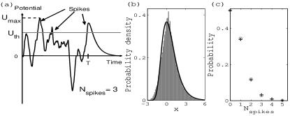
Figure 1: (a) Example of voltage traces $U(t)$. (b) Probability density of the rescaled maximal potential $x$ as defined in eq. (4) with a fitted scale factor $\beta$. (c) Probability of $N_{\text{spikes}}$. The Line in (b) is a standard Gumbel law. In (c) circles indicate the theoretical Poisson law. Data was measured with $K=400,\ \alpha=1.68,\ N=500$ and 34 samples.

In this Letter we present a theoretical study of the computational power of the Tempotron. We focus on the standard task of classifying a batch of $P=\alpha N$ random patterns, where $\alpha$ denotes the number of patterns per input synapse. For each pattern, the timings of the input spikes from each input neuron are randomly chosen from independent Poisson processes with rate $\frac{1}{T}$, where $T$ is the duration of the input patterns, and the desired output, $y=\pm 1$, is randomly and independently chosen with equal probabilities. A solution to the classification problem is a set of synaptic weights $\{\omega_{i}\}$ that yields a correct classification of all $P$ patterns. We will address several fundamental questions. First, numerical simulations based on a simple error-correcting on-line learning algorithm suggest that the capacity of the IF neuron namely, the maximal number of patterns per synapse, $\alpha_{c}$, which, with high probability (approaching 1 for large $N$), can be correctly classified is independent of the number of input synapses (gutig2006tnl, ); however, an analytical proof for this property has been lacking. Secondly, it is important to understand how the computational capabilities of the neuron depend on the various time scales in the dynamics of the system. Finally, our study highlights the complex geometric structure of the space of solutions for $\alpha<\alpha_{c}$, similar to the one arising in other hard computational problems, such as learning in multilayered neural networks (engel2001sml, ) or random combinatorial optimization (Monasson20071, ; mezard2009information, ).

Our theoretical analysis, presented below, shows that a fundamental parameter is the pattern duration, $T$, relative to the neural time scales,

$$K=\frac{T}{\sqrt{\tau_{s}\tau_{m}}}\ .$$ (2)

The properties of the Tempotron can be most easily understood, when both $N$ and $K$ are large, with $N\gg K$. This limit is biologically sensible if we consider a neuron with $N\sim 10^{3}$ synapses, inputs that are presented for $T\sim 100-1000$ milliseconds, and constants $\tau_{s}\sim 1-10$, $\tau_{m}\sim 10-100$ milliseconds. We predict that, for any fixed $K$, the capacity is independent of $N$ in the large $N$ limit. Furthermore, the capacity grows with $K$ as

$$\alpha_{c}=\frac{\ln\ln K}{2\ln 2}\ .$$ (3)

The convergence of the capacity to this expression is slow, requiring that $\sqrt{\ln K}\gg 1$. Nevertheless, this result has several qualitative implications. Equation (3) implies that the capacity of the Tempotron is not bounded as $K$ increases, and may exceed the capacity of the well-known Perceptron model ($\alpha_{c}=2$ (gardner1987msc, )) whose architecture is similar to the Tempotron. Note that when $K$ is $O\left(N\right)$, the few input spikes that arrive within a single decision time window, $T/K$, do not carry sufficient information to classify the patterns. We therefore expect that for any fixed $N$, $\alpha_{c}$ is a non monotonic function of $K$ while the value of $K$ that maximizes the capacity increases with $N$, as implied by (3). This prediction is corroborated by numerical simulations in Fig. 2a. Interestingly, according to eq. (2), the performance should be sensitive also to the short time behavior of the kernel as confirmed by the simulations of Fig. 2b. This short time behavior determines how fast can the membrane potential change significantly. The faster this cange can be, the easier it is to distinguish between inputs that arrive within a short interval of time.

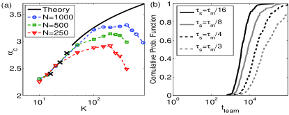
Figure 2: (a) Capacity $\alpha_{c}$ of the Tempotron vs. $K$. Lines with symbols show results from the learning algorithm of (gutig2006tnl, ). The solid line shows the large–$K$ theory (3), with an additive constant ($\alpha_{c}=\left(\ln\ln K\right)/2\ln 2+\alpha_{0}$, with $\alpha_{0}=2.58$) fitted to the predictions of the replica method for the discrete Tempotron for $K^{\text{discrete}}=2,3,4$ ($\times$ symbols). To compare the theory of the discrete Tempotron with the simulation results of the continuous time Tempotron we used $K^{\text{discrete}}=K/8$. (b) Distribution of learning times for different $\tau_{s}$, and for fixed $\tau_{m}=T/25$, $\alpha=2.6$ and $N=1000$. As $\tau_{s}$ decreases so does the mean learning time, indicating that |$\alpha-\alpha_{c}|$ has increased, as predicted by eqs. (2) and (3).

In the Perceptron model, the solution space for a given classification task is a convex volume, which shrinks in size and ultimately vanishes as $\alpha$ approaches the capacity, $\alpha_{c}$. The overlap between two typical solutions, $q_{0}$, defined by the inner product between their normalized weight vectors, approaches $1$ at the critical capacity (gardner1987msc, ). Our theory reveals that the solution space of the Tempotron is of a strikingly different nature. First, the overlap between two Tempotron weight vectors that solve the random classification problem, $q_{0}$, approaches zero in the $K\gg 1$ limit, for every $\alpha<\alpha_{c}$. Secondly, the solution space is connected for small $\alpha$ only. For larger values of $\alpha$, still far below capacity, the solution space breaks into a large number of small disconnected clusters, spread across the entire weight space. The overlap between solutions within the same cluster, $q_{1}$, is close to $1$, while two randomly chosen solutions are likely to lie in different clusters and have overlap $q_{0}\approx 0$. Simulations making use of the learning algorithm of (gutig2006tnl, ) support this picture. The overlap between two solutions obtained from two different initial weight vectors vanishes for all values of $\alpha$ (Fig. 3a). To probe the overlap between solutions in the same cluster, we performed a random walk in solution space (barkai1992bsm, ), starting from a solution found by the Tempotron learning algorithm and rejecting the random walk step attempts if they lead to a weight vector that is not a valid solution. The auto-correlation function of this random walk drops exponentially fast to zero for small $\alpha$, indicating that the solutions space is connected, and hardly decays for higher $\alpha(<\alpha_{c})$, as expected for a clustered solution space, (Fig. 3b).

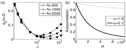
Figure 3: (a) Overlap between randomly chosen solutions, $q_{0}$, at $\alpha=2$ as a function of $K$. (b) Auto-correlation function $q_{AC}(\Delta t)\equiv\langle\hat{\omega}(t)\cdot\hat{\omega}(t+\Delta t)\rangle$ of a random walk inside a connected volume in solutions space for $K=150$ and $N=500$.

The above results are surprising and counter-intuitive since they imply that even close to capacity, IF neurons with very different weights can perform exactly the same classification, whereas IF neurons with high degree of similarity in their weight vectors will typically fail to solve the same task. To understand these properties we consider a Tempotron whose $N$ weights are random variables drawn from any probability distribution with finite first two moments. With no loss of generality we may choose the mean and variance of the weights to ensure that $U(t)$ has zero mean and unit variance. The threshold potential, $U_{\text{th}}$, is such that a random pattern is classified by each Tempotron as $\pm 1$ with equal probabilities, i.e., $U_{\text{th}}$ is the median value of the distribution of the maximum of $U(t)$ over time, $U_{\text{max}}$. The synaptic potential $U(t)$ induced by a random input pattern approaches, in the large $N$ limit, a temporally correlated Gaussian distribution. We use extreme value theory (EVT) of Gaussian processes to evaluate the statistics of $U_{\text{max}}$ (leadbetter1983extremes, ). According to EVT, $U_{\text{max}}$ can be written as

$$U_{\text{max}}=U_{\text{th}}+\beta(x+\ln\ln{2})$$ (4)

where $x$ obeys the Gumbel density distribution $G(x)=\exp\left(-x-\exp(-x)\right)$, whose median is $-\ln\ln 2$. The scale factor is $\beta=1/\sqrt{2\ln{K}}+O\left(1/\ln{K}\right)$ and the threshold is $U_{\text{th}}=\sqrt{2\ln{K}}+O\left(1/\sqrt{\ln{K}}\right)$, where $K=T\sqrt{\left|\frac{d^{2}C(0)}{dt^{2}}\right|}$ and $C(t)=\left\langle U\left(t^{\prime}\right)U\left(t^{\prime}+t\right)\right\rangle$ is the auto-correlation function of $U(t)$. These results are valid provided that $C(t)$ decays to zero at long times and $K$ is large . Note that for a kernel $u(t)$ in eq. (1) of the form of difference of exponentials, $K$ takes the value of eq. (2).

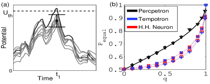
Figure 4: (a) Time traces of the potentials of a Tempotron with random weights, $U_{1}(t)$ (bold line), and of seven other Tempotrons, $U_{2}(t)$ (gray lines), having overlap $q=.8$ with the first one. The pattern is the same for all Tempotrons, and is classified as $+1$ by the first Tempotron: $U_{1}\left(t\right)$ is maximal in $t_{1}$, and exceeds $U_{\text{th}}$. The error bar is centered in $t=t_{1},\bar{U}_{2}=q\,U_{1}\left(t_{1}\right)$, and has height $\sqrt{1-q^{2}}$. Parameters are $K=100,\ N=1000$. (b) Probability that 2 neurons will classify a random pattern in the same manner, $P_{\text{equal}}$, vs. overlap between their weight vectors, $q$, for the Perceptron (theory and simulations in black), the Tempotron (blue $\times$ and $+$ symbols correspond, respectively, to $K=100$ and $K^{\prime}=4K=400$) and the Hodgkin-Huxley (red squares and circles correspond to $T=1.5\ \text{sec}$ and $T^{\prime}=4T=6\ \text{sec}$ respectively [13]) models.

We now consider two such Tempotrons, with an overlap $q$ between their two weight vectors. Let us choose a pattern that is classified as $+1$ by the first and denote by $t_{1}$ the time at which its potential reaches its maximum value $U_{1}>U_{\text{th}}$. Let us denote the postsynaptic potential of the second Tempotron at time $t_{1}$ by $U_{2}$. Conditioned on $U_{1}$, the probability distribution of $U_{2}$ is Gaussian with mean $\overline{U}_{2}=q\,U_{1}$ and standard deviation $\sigma=\sqrt{1-q^{2}}$. According to (4) $U_{1}$ is close to $U_{\text{th}}$, and we may approximate $U_{\text{th}}-\overline{U}_{2}\simeq(1-q)\sqrt{2\ln{K}}$. Thus, as long as $1-q\gg\frac{1}{\ln K}$, the typical fluctuations of $U_{2}$ which are of $O(\sigma)$ are much smaller than the gap between $\overline{U}_{2}$ and the threshold (Fig. 4a); hence $U_{2}$ is very likely smaller than $U_{\text{th}}$. This implies that the overall probability that the second Tempotron’s potential crosses the threshold at any time remains close to $1/2$, unless

$$q\geq 1-O\left(\frac{1}{\ln K}\right)\ .$$ (5)

Thus, two Tempotrons are likely to agree on their classifications of a random pattern only if the overlap in their synaptic weights is close to 1. This result is confirmed by the simulations shown in Fig. 4b. We also present the simulation results for the Hodgkin Huxley model [13], a classical biophysical model for spike generation. Interestingly, despite its complex dynamics, the classification pattern of a pair of Hodgkin-Huxley neurons is similar to that of the Tempotron, indicating that this behavior does not depend on the details of the spike generation but on the summation of input spikes within temporal windows. In contrast, in the case of the Perceptron, which lacks temporal windows, the probability that two weight vectors agree on their classification increases roughly linearly with their overlap, $q$ (Fig. 4b). The above result provides a qualitative explanation of the clustered nature of the solution space. Consider one solution to the classification task. Very similar weight vectors, with overlaps larger than $1-O\left(1/\ln K\right)$ are likely to be solutions, too, and compose a very small connected cluster of solutions around the first solution. On the other hand having any positive overlap smaller than this scale, does not provide significant advantage in terms of classification error. Hence, entropy pressure for decreasing the overlap wins, yielding a vanishingly small overlap $q_{0}$ between two typical solutions.

The fact that $q_{0}$ is small for all $\alpha$ has important consequences. First, $q_{0}$ in general measures the strength of the correlations between the solution weight vector and individual quenched learnt patterns. Small $q_{0}$ implies, therefore, that the statistics of the potential after learning is approximately Gaussian with variance and mean which are governed by the requirement that random patterns induce spiking with probability $\frac{1}{2}$. As described above, this implies that the distribution of $U_{\text{max}}$ of learnt patterns has a Gumbel shape. Furthermore EVT predicts that the number of threshold crossings in a pattern of duration $T$, $N_{\text{spikes}}$, obeys a Poisson distribution with a mean rate $r=\frac{\ln{2}}{T}$, consistent with a $\frac{1}{2}$-probability of firing within time $T$ (leadbetter1983extremes, ). These predictions are confirmed by numerical simulations shown in Fig. 1b,c.

EVT provides a basis for estimating the value of the capacity. Drawing on analogy from the replica calculations ((monasson1994dsa, ) and below), we estimate the entropy of clusters in the solution space, $S_{cl}$, through $S_{cl}=(\ln{V}-\ln{V_{cl}})/N$, where $V$ and $V_{cl}$ are, respectively, the total volume of solutions and the typical volume of one cluster. As $q_{0}\simeq 0$, $V$ is simply the product of the probabilities that the Gaussian potential $U$ crosses the threshold for each $+1$ pattern and does not do so for each $-1$ pattern: $V=\left(\frac{1}{2}\right)^{N\alpha}$. Assuming that the typical cluster is of ’compact’ shape, its volume is given by $V_{cl}=(1-q_{1})^{N/2}$ where $q_{1}$ is the typical overlap between solutions within the cluster and scales according to eq. (5) as $1-q_{1}=O(1/\ln K)$. We therefore obtain,

$$S_{cl}\simeq\frac{1}{2}{\ln\ln K}-\alpha\,\ln 2\ .$$ (6)

Classifications are possible as long as $S_{cl}>0$, which yields the capacity (3).

The above results are supported by an independent statistical mechanical study of a simpler model, the discrete Tempotron (gutig2006tnl, , Sup. Mat.), where time is discrete, $t=\ell\,\tau$, $\ell=1,2,3,...$, and the potential $U_{\ell}$ is the sum of the synaptic weights $\omega_{i}$, multiplied by the number of spikes emitted by input $i$ in the time-bin $\ell$. The patterns to be classified are associated an internal representation (IR), which consists of the set of time-bin indices $\ell$ such that $U_{\ell}>U_{th}$. The weight vectors implementing the same IR form a convex domain of solutions. As the entire solution space is not expected to be convex, calculating its volume is a difficult task. Instead, following (monasson1994dsa, ; engel2001sml, ), we have calculated the average value of the logarithm of the number of typical implementable IR domains, $S_{IR}$, as a function of $\alpha$. The calculation, based on the replica method, involves two overlaps: the intra-overlap of a domain, $q_{1}^{IR}$, and the inter-overlap between two domains, $q_{0}^{IR}$. When $K=\frac{T}{\tau}\gg 1$ and $\alpha\gg\frac{1}{\ln K}$, we find $q_{0}^{IR}\sim\frac{\alpha}{\ln K}$, $1-q_{1}^{IR}\sim\frac{1}{\alpha^{2}\ln K}$, and $S_{IR}$ given by the right-hand side of (6). Hence $q_{0}^{IR}$ vanishes as long as $\alpha\ll\ln K$, and the scaling of $q_{1}^{IR}$ is compatible with $q_{1}$ given by EVT. This calculation also enables us to estimate the capacity at finite $K$ (See Fig. 2a). The similarity between quantities defined in terms of connected clusters of solutions, and those defined in terms of IR domains is a consequence of the binary character of the overlaps in the large $K$ limit. For the same reason, further effects of replica symmetry breaking should affect only subleading corrections to $\alpha_{c}$. Numerical simulations show that the discrete Tempotron behaves very similarly to the continuous time Tempotron (Data not shown). This implies that the computational capability of the Tempotron is not sensitive to the detailed shape of the temporal integration.

In conclusion, we have presented a theory of the computational capacity of a neuron that performs classification of inputs by integrating incoming spikes in space and time and generates its decision via threshold crossing. Importantly, the Tempotron is not constrained to fire at a given time in response to a target pattern. Thus, by adjusting the timing of its output spikes, the Tempotron can choose the spatio-temporal features that will trigger its firing for each target pattern. Despite the simplicity of its architecture and dynamics, this property of the Tempotron decision rule yields a rather complex structure of the solution space and accounts for the superior performances of the Tempotron compared to the Perceptron and to Perceptron-based models for learning temporal sequences (bressloff1992perceptron, ) which specify the desired times of the output spikes.

- (1) M. Minsky and S. Papert, Perceptrons: expanded edition (MIT Press Cambridge, MA, USA, 1988)
- (2) E. Gardner, Europhys. Lett. 4, 481 (1987)
- (3) R. Johansson and I. Birznieks, Nat. Neuro. 7, 170 (2004)
- (4) T. Gollisch and M. Meister, Science 319, 1108 (2008)
- (5) R. Gütig and H. Sompolinsky, Nat. Neuro. 9, 420 (2006)
- (6) In all the numerical results presented here we have used except in Fig. 2b
- (7) In this work effects of potential reset after a spike are not relevant
- (8) A. Engel and C. Broeck, Statistical mechanics of learning (Cambridge Univ Pr, 2001)
- (9) R. Monasson, in Complex Systems, Les Houches, Vol. 85, edited by J.-P. Bouchaud, M. Mezard, and J. Dalibard (Elsevier, 2007) pp. 1 – 65
- (10) M. Mezard and A. Montanari, Information, physics, and computation (Oxford University Press, USA, 2009)
- (11) E. Barkai, D. Hansel, and H. Sompolinsky, Phys. Rev. A 45, 4146 (1992)
- (12) M. Leadbetter, G. Lindgren, and H. Rootzén, Extremes and related properties of random sequences and processes (Springer, NY, USA, 1983)
- (13) See EPAPS Document No. [] for Supplementary Material.
- (14) R. Monasson and D. O’Kane, Europhys. Lett. 27, 85 (1994)
- (15) P. Bressloff and J. Taylor, Journal of Physics A: Mathematical and General 25, 4373 (1992)