Adaptive image ray-tracing for astrophysical simulations

Abstract

A technique is presented for producing synthetic images from numerical simulations whereby the image resolution is adapted around prominent features. In so doing, adaptive image ray-tracing (AIR) improves the efficiency of a calculation by focusing computational effort where it is needed most. The results of test calculations show that a factor of $\mathrel{\hbox to0.0pt{\lower 3.0pt\hbox{$\sim$}\hss}\raise 2.0pt\hbox{$>$}}4$ speed-up, and a commensurate reduction in the number of pixels required in the final image, can be achieved compared to an equivalent calculation with a fixed resolution image.

1 Introduction

Numerical models, such as hydrodynamical simulations, have become a popular tool in astrophysical research. A common approach to extracting observable quantities from a numerical simulation is to trace the path of a ray through the simulation domain and sum-up the value of some quantity at discrete intervals. Typically this is done to integrate the column density through the simulation domain or to solve the equation of radiative transfer to determine the emergent intensity of emission. Synthetic images produced via ray-tracing can be very useful for constraining model parameters, and examples of this can be found in a wide range of astrophysical studies, e.g. symbiotic recurrent nova (Orlando et al. 2009; Drake & Orlando 2010), active galactic nuclei (Brüggen et al. 2009; Falceta-Gonçalves et al. 2010), star formation (Kurosawa et al. 2004; Krumholz et al. 2007; Parkin et al. 2009; Offner & Krumholz 2009; Peters et al. 2010; Douglas et al. 2010), jets (Sutherland & Bicknell 2007; Bonito et al. 2007; Saxton et al. 2010), starburst galactic winds (Cooper et al. 2008), and colliding winds binaries (Pittard & Dougherty 2006; Pittard & Parkin 2010). However, one drawback with using a fixed resolution image (i.e. same pixel size at all points) is that a large amount of computational effort can be expended on essentially blank regions as features of interest rarely fill an entire image.

For example, in modern hydrodynamic simulations the grid/particle resolution is often adapted to features in the flow. In grid-based codes this is achieved using adaptive-mesh refinement (AMR - e.g. Berger & Oliger 1989), whereas smoothed-particle hydrodynamics (SPH - see Monaghan 1992) is inherently adaptive. When producing an image the resolution must be sufficiently high to ensure that the smallest scales of the simulation are well sampled. Yet there may be regions of a simulation which do not warrant such a high level of sampling. Furthermore, a ray which passes through a highly refined region of the simulation domain may not necessarily hold much useful information once it exits the grid. For instance, regions of high intrinsic emission may be heavily absorbed such that the emergent intensity is negligible. With these details in mind, as well as the fact that as the computational requirements of simulations rise there will be an associated increase in the memory required by datasets, more efficient approaches to extracting observable quantities are warranted.

This letter describes a method for adapting the resolution of a ray-traced image to the feature(s) of interest. In so doing the efficiency of a calculation is significantly improved. Adaptive image ray-tracing (AIR) takes advantage of the varying simulation resolution and magnitude of the extracted information encountered by a ray. In essence, the advantages that adaptive mesh refinement (AMR) has brought to grid-based hydrodynamical simulations are incorporated into ray-tracing. The process is in a sense the reverse of super-sampling (e.g. Whitted 1980; Genetti & Gordon 1993), where instead of averaging over multiple rays, a single ray is subdivided. Test calculations show that, compared to a fixed resolution image, AIR provides an appreciable speed-up and a reduced number of pixels for the resulting image. The remainder of this letter is structured as follows: in § 2 the AIR technique is outlined, § 3 presents results from test calculations, and conclusions are presented in § 4.

2 Adaptive image ray-tracing

The basic principle behind producing a ray-traced image is to first discretize the plane of the sky into a uniform array of pixels and then follow the path of a ray for each respective pixel. The AIR technique builds on this by taking an initially low resolution image and then adapting (increasing) the resolution around sufficiently prominent features of interest. This leads to a far more efficient calculation as computational effort is concentrated on producing an image of a desired variable(s). The structure of the AIR scheme is as follows:

1. Construct base image: After reading in the simulation file the base image resolution can be determined and the initial image constructed. As a guideline, the base image resolution can be set to sample the lowest resolution regions of the simulation domain. For example, for an AMR simulation setting the base image resolution equivalent to the base grid of the simulation is adequate.

2. Ray-trace: Extract the desired information from the simulation domain by following the path of rays for each respective pixel.

3. Scan the image to check if refinement is required: This is a relatively straightforward process of calculating the truncation error for a given pixel. The step in resolution between adjacent image pixels is prevented from being more than one refinement level - this ensures that the edges of features are well sampled.

4. Refine pixels: The pixels selected by the truncation error check should now be refined. The $ij$ indexing of pixels cannot be preserved and therefore a heirarchical tree structure is required. Hence, during this step the book-keeping must be performed and information about the neighbours, parent, and children of a pixel updated.

5. Loop: Repeat steps 2-4 until features in the image have been captured to the desired resolution and no more pixel refinement is required. For instance, the image resolution need not exceed that of the simulation.

6. Integrate quantities and output: Once the final image has been constructed integrated quantities can be determined. An example of this would be broadband images in a given frequency/energy range. The sharpness of edges in the image can be improved by incorporating a super-resolution algorithm to interpolate between adjacent pixels of differing resolution (e.g. Chu et al. 2009). Following this, the final step is to output the image.

As a note of caution, when calculating an integrated spectrum from an image it is necessary to store the spectrum for each individual pixel until the calculation is finished. This can lead to a prohibitive overhead in memory requirements. However, this problem can be alleviated by writing the spectrum for each pixel to temporary files during the calculation.

Considering that the majority of the computational effort is expended on the ray-tracing step, effective speed-up can be achieved by parallelizing the AIR scheme on this step alone. This would involve distributing the list of pixels across processors during each ray-tracing sweep and then gathering the information for the refinement check. Alternatively, it is conceivable that such a code could be manufactured by taking an existing fixed-image ray-tracing code and interfacing it with a parallel AMR library, e.g. PARAMESH (MacNeice et al. 2000), CHOMBO (Colella et al. 2009), DAGH (Parashar & Browne 1995), SAMRAI (Wissink et al. 2001). For instance, AMR libraries typically have in-built functionality for parallel grid management, e.g.. refinement, cell list book-keeping, interprocessor communication, and load balancing. Therefore, ray-tracing could be handled on a pixel-by-pixel basis using an existing fixed-image ray-tracing code, and the parallel computation and grid management could be dealt with by functions available in the AMR library. The process would be akin to the initial refinement sweep performed in a grid-based hydrodynamics code, with the difference that instead of populating a refined cell using the simulation initial conditions a refined pixel is populated using the results from a ray-tracing calculation.

3 An example application

To demonstrate the advantages of using AIR compared to ray-tracing with a fixed resolution image, calculations have been performed for a test case. For this purpose a ring of hot gas residing at the centre of a three-dimensional box has been simulated. The ring is aligned with the $yz$-plane, has a constant thickness $w=1\times 10^{17}\;{\rm cm}$, and has inner and outer radii of $r_{\rm i}=3.5\times 10^{17}\;{\rm cm}$ and $r_{\rm o}=4\times 10^{17}\;{\rm cm}$, respectively. The box has dimensions $x=y=z=\pm 5\times 10^{17}\;{\rm cm}$. The gas density (g cm^-3),

$$\rho=\left\{\begin{array}[]{lll}\beta r_{yz}^{-2}&;r_{\rm i}\leq r_{yz}\leq r_{\rm o},&|x|<w/2\\ 1\times 10^{-25}\;{\rm g~{}cm^{-3}}&;{\rm otherwise}\\ \end{array}\right.$$ (1)

where $\beta=2.5\times 10^{-9}\;{\rm g~{}cm^{-1}}$ and $r_{yz}=\sqrt{y^{2}+z^{2}}$. The gas temperature is $10^{8}\;$K and $10^{4}\;$K inside and outside of the ring, respectively.

The ring and the box are modelled on an AMR grid constructed using the FLASH code v3.1.1 (Fryxell et al. 2000; Dubey et al. 2009), which operates with the PARAMESH block-structured AMR package (MacNeice et al. 2000). The coarse grid consists of $4^{3}$ blocks containing $8^{3}$ cells. Refinement is performed on density and temperature using 4 nested grid levels such that the effective resolution is $512^{3}\;$cells.

For the AIR calculations the base image has a resolution of $32^{2}$ pixels and 4 nested levels of image refinement were used, giving an effective image resolution of $512^{2}$ pixels (equivalent to a fixed image calculation). The refinement check is performed on the integrated 1-10 keV intrinsic X-ray flux using a modified second-derivative interpolation error estimate (Löhner 1987). This is essentially a second-order central difference normalized by the sum of first-order forward and rearward differences, which in one dimension on a uniform mesh is,

$$\xi_{i}=\frac{|p_{i+1}-2p_{i}+p_{i-1}|}{|p_{i+1}-p_{i}|+|p_{i}-p_{i-1}|}$$ (2)

where $\xi$ is the truncation error, $p$ is the value of the parameter on which image refinement is desired in pixel $i$ (e.g. X-ray flux). The multidimensional generalization of Eq. 2 is found by taking all cross derivatives, which leads to,

$$\xi_{ij}=\left(\frac{\sum\limits_{uv}\left(\frac{\partial^{2}p}{\partial x_{u}\partial x_{v}}\Delta x_{u}\Delta x_{v}\right)^{2}}{\sum\limits_{uv}\left[\left(|\frac{\partial p}{\partial x_{u}}|_{i_{u}+1/2}+|\frac{\partial p}{\partial x_{u}}|_{i_{u}-1/2}\right)\Delta x_{u}\right]^{2}}\right)^{\frac{1}{2}}$$ (3)

where $u$ and $v$ are the image coordinates with indices $i$ and $j$, respectively, and $\Delta x_{a}$ is the separation of nodes in the coordinate direction $a$. The partial derivatives are determined at pixel centres and the sums are carried out over coordinate directions. If $\xi_{ij}\geq\xi_{\rm crit}$ then the pixel is marked for refinement. Determining the optimal value for $\xi_{\rm crit}$ for a given application requires some experimentation; for the test case values of $\xi_{\rm crit}>0.01$ are effective at refining the ring whilst maintaining efficiency. However, further tests performed on images which contain more structure and varying degrees of contrast reveal that $\xi_{\rm crit}\simeq 0.5$ is a more appropriate start point. Löhner’s error estimate is useful because it is bounded (i.e. $0\leq\xi<1$) so that a preset refinement tolerance can be employed. It is also dimensionless, meaning that more than one image parameter can be used to check for refiment without encountering dimensioning problems.

To calculate the intrinsic X-ray emission we assume solar abundances and use emissivities for optically thin gas in collisional ionization equilibrium obtained from look-up tables calculated from the MEKAL plasma code (Kaastra 1992; Mewe et al. 1995).

The test problem places the observer viewing the ring face-on (parallel to the $x$-axis) at a distance of 1 kpc and traces rays through the hydrodynamic grid to calculate the intrinsic 1-10 keV flux. For comparison, calculations have been performed with a fixed image and with AIR using $\xi_{\rm crit}=0.2$, 0.5, and 0.8 (Fig. 1 and Table 1). The fixed image calculation is constrained by the fact that image pixels must be small enough to sample the highest refined regions of the hydrodynamic grid, hence the resolution must be $512\times 512\;$pixels. In contrast, the AIR calculation begins with a base image of $32\times 32\;$pixels then locates the feature of interest (the ring in this case) and increases the image resolution respectively. This leads to far fewer pixels being used and thus a more efficient calculation. For example, the $\xi_{\rm crit}=0.8$ AIR calculation takes $\sim 1/7$ the time and requires $\sim 1/12$ the image pixels, with a negligible error in the integrated flux of 0.01%.

As a approximate rule of thumb, AIR will reduce the calculation time and pixel consumption by a factor of roughly the inverse of the image filling factor, e.g. in the test calculation the ring fills $\sim 1/8$ of the image.

Table 1: Adaptive image ray-tracing test calculation results. $\xi_{\rm crit}$ is the critical error estimate used to flag pixels for refinement (see Eq 3), $F_{\rm X}$ is the intrinsic 1-10 keV flux, $t$ is the time taken for the calculation. The error is calculated as $(F_{\rm Xexact}-F_{\rm Xray})/F_{\rm Xexact}$, where $F_{\rm Xexact}=1.399586\times 10^{-19}\;{\rm erg~{}s^{-1}~{}cm^{-2}}$ is the intrinsic flux summed from the hydrodynamic grid and $F_{\rm Xray}$ is the ray-traced value for a given calculation.

Calculation	$\xi_{\rm crit}$	Fractional Error	$t$	Pixels
			(s)
Fixed	$-$	$\sim 0.$	9604	262144
AIR	0.2	$2\times 10^{-6}$	2627	40512
AIR	0.5	$1\times 10^{-4}$	1374	23384
AIR	0.8	$1\times 10^{-4}$	1339	22748

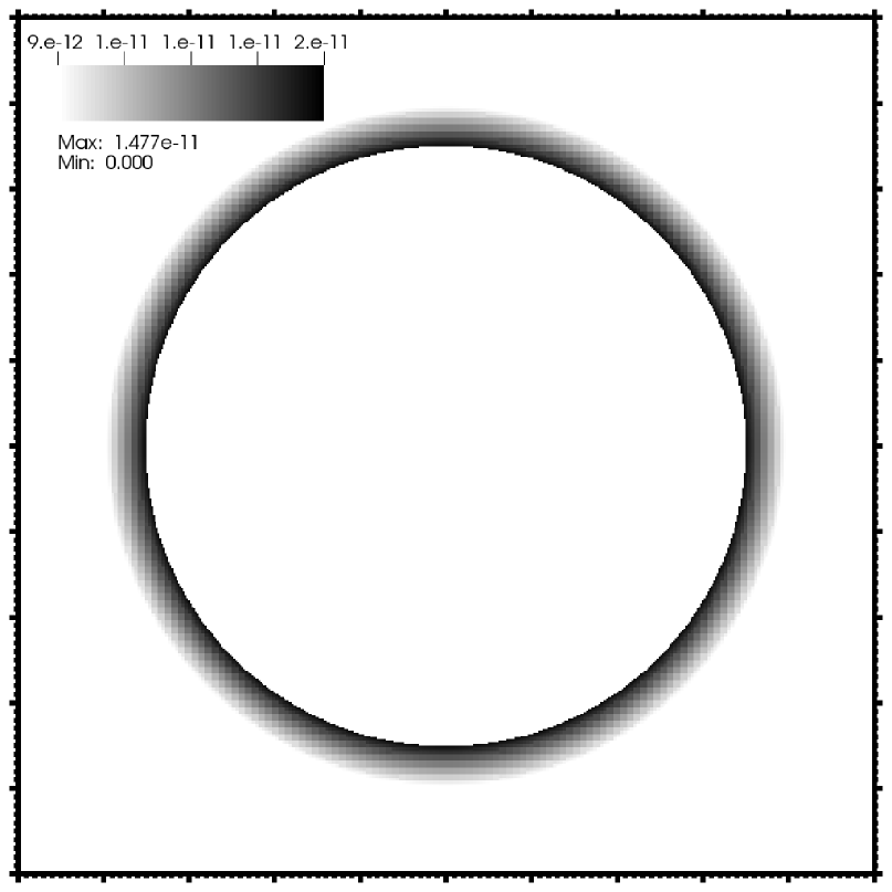
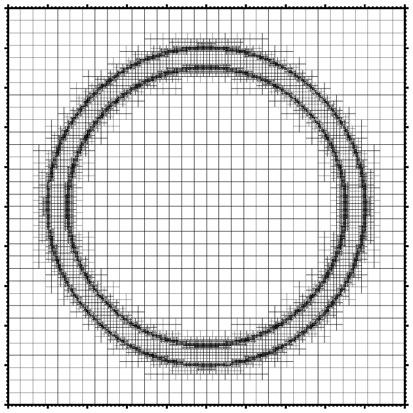
Figure 1: Results from the $\xi_{\rm crit}=0.8\;$ test calculation showing intrinsic 1-10 keV X-ray flux (top panel) and the image pixel mesh (lower panel). The images show a spatial extent of $u=v=\pm 5\times 10^{17}\;{\rm cm}$ - large tick marks correspond to $1\times 10^{17}\;{\rm cm}$. Note that for the adopted viewing angles $(u,v)=(y,z)$. For further details of the test calculations see § 3 and Table 1.

4 Conclusions

A method has been presented for adaptively increasing the resolution of a ray-traced image around prominent features of interest. An initially low resolution image is scanned and relevant pixels are refined to increase the image resolution. The results of test calculations show that considerable speed-up (a factor of $\sim 4-7$), and a commensurate reduction in the number of pixels required for the final image (a factor of $\sim 6-11$), can be achieved compared to an equivalent calculation with a fixed resolution image. In conclusion, adaptive image ray-tracing (AIR) improves the efficiency of a calculation by focusing computational effort on extracting desired information.

Acknowledgements

This work was supported by a PRODEX XMM/Integral contract (Belspo). The author thanks Julian Pittard and Andrii Elyiv for insightful discussions and the anonymous referee for helpful comments which improved the presentation of this paper. This research has used software which was in part developed by the DOE-supported ASC/Alliance Center for Astrophysical Thermonuclear Flashes at the University of Chicago.

References

- Berger & Oliger (1989) Berger, M. J. & Oliger, J. 1989, Journal of Computational Physics, 53, 484
- Bonito et al. (2007) Bonito, R., Orlando, S., Peres, G., Favata, F., & Rosner, R. 2007, A&A, 462, 645
- Brüggen et al. (2009) Brüggen, M., Scannapieco, E., & Heinz, S. 2009, MNRAS, 395, 2210
- Chu et al. (2009) Chu, J., Liu, J., Qiao, J., Wang, X., & Li, Y. 2009, arXiv:0903.3995
- Colella et al. (2009) Colella, P., et al. 2009, Chombo Software Package for AMR Applications (unpublished)
- Cooper et al. (2008) Cooper, J. L., Bicknell, G. V., Sutherland, R. S., & Bland-Hawthorn, J. 2008, ApJ, 674, 157
- Douglas et al. (2010) Douglas, K. A., Acreman, D. M., Dobbs, C. L., & Brunt, C. M. 2010, MNRAS, 407, 405
- Drake & Orlando (2010) Drake, J. J. & Orlando, S. 2010, ApJ, 720, 195
- Dubey et al. (2009) Dubey, A., Reid, L. B., Weide, K., Antypas, K., Ganapathy, M. K., Riley, K., Sheeler, D., & Siegal, A. 2009, arXiv:0903.4875
- Falceta-Gonçalves et al. (2010) Falceta-Gonçalves, D., Caproni, A., Abraham, Z., Teixeira, D. M., & de Gouveia Dal Pino, E. M. 2010, ApJL, 713, L74
- Fryxell et al. (2000) Fryxell, B., et al. 2000, ApJS, 131, 273
- Genetti & Gordon (1993) Genetti, J. & Gordon, D. 1993, Graphics Interface, pp 70–77
- Kaastra (1992) Kaastra, J. S. 1992, Internal SRON-Leiden Report
- Krumholz et al. (2007) Krumholz, M. R., Klein, R. I., & McKee, C. F. 2007, ApJ, 665, 478
- Kurosawa et al. (2004) Kurosawa, R., Harries, T. J., Bate, M. R., & Symington, N. H. 2004, MNRAS, 351, 1134
- Löhner (1987) Löhner, R. 1987, Comp. Meth. App. Mech. Eng., 61, 323
- MacNeice et al. (2000) MacNeice, P., Olson, K. M., Mobarry, C., deFainchtein, R., & Packer, C. 2000, Comp. Phys. Comm., 126, 330
- Mewe et al. (1995) Mewe, R., Kaastra, J. S., & Liedahl, D. A. 1995, Legacy, 6, 16
- Monaghan (1992) Monaghan, J. J. 1992, ARA&A, 30, 543
- Offner & Krumholz (2009) Offner, S. S. R. & Krumholz, M. R. 2009, ApJ, 693, 914
- Orlando et al. (2009) Orlando, S., Drake, J. J., & Laming, J. M. 2009, A&A, 493, 1049
- Parashar & Browne (1995) Parashar, M. & Browne, J. C. 1995, Proceedings of the International Conference for High Performance Computing
- Parkin et al. (2009) Parkin, E. R., Pittard, J. M., Hoare, M. G., Wright, N. J., & Drake, J. J. 2009, MNRAS, 400, 629
- Peters et al. (2010) Peters, T., Banerjee, R., Klessen, R. S., Mac Low, M., Galván-Madrid, R., & Keto, E. R. 2010, ApJ, 711, 1017
- Pittard & Dougherty (2006) Pittard, J. M. & Dougherty, S. M. 2006, MNRAS, 372, 801
- Pittard & Parkin (2010) Pittard, J. M. & Parkin, E. R. 2010, MNRAS, 403, 1657
- Saxton et al. (2010) Saxton, C. J., Wu, K., Korunoska, S., Lee, K., Lee, K., & Beddows, N. 2010, MNRAS, 405, 1816
- Sutherland & Bicknell (2007) Sutherland, R. S. & Bicknell, G. V. 2007, ApJS, 173, 37
- Whitted (1980) Whitted, T. 1980, Communications of the ACM, 23, 343
- Wissink et al. (2001) Wissink, A. M., Hornung, S. R., Kohn, S. R., Smith, S. S., & Elliott, N. S. 2001, SC01 Proceedings