Comparison of Energies Between Eruptive Phenomena and Magnetic Field in AR 10930

Abstract

We present a study comparing the energy carried away by a coronal mass ejection (CME) and the radiative energy loss in associated flare plasma, with the decrease in magnetic free energy during a release in active region NOAA 10930 on December 13, 2006 during the declining phase of the solar cycle 23. The ejected CME was fast and directed towards the Earth with a projected speed of $\sim$1780 km s^-1 and a de-projected speed of $\sim$3060 km s^-1. We regard these as lower and upper limits for our calculations. It was accompanied by an X3.4 class flare in the active region. The CME carried (1.2–4.5)$\times$10³² erg (projected-deprojected) of kinetic and gravitational potential energy. The estimated radiative energy loss during the flare was found to be 9.04$\times$10³⁰ erg. The sum of these energies was compared with the decrease in measured free magnetic energy during the flare/CME. The free energy is that above the minimum energy configuration and was estimated using the magnetic virial theorem. The estimated decrease in magnetic free energy is large, 3.11$\times$10³² erg after the flare/CME compared to the pre-flare energy. Given the range of possible energies we estimate that 50–100% of the CME energy arose from the active region. The rest of the free magnetic energy was distributed among the radiative energy loss, particle acceleration, plasma and magnetic field reorientation.

1 Introduction

Sunspots are the harbor for solar magnetic fields. Energetic phenomena like solar flares occurring in sunspots derive their energy from the active region magnetic fields. It is generally believed that coronal mass ejections (CME) which are associated with active regions obtain the majority, if not all of, their energy from these magnetic structures. The magnetic energy stored in the twisted magnetic fields is released within a few minutes during these energetic events and is of the order of 10³² erg. The majority of the energy released is carried away by the CME mostly in the form of kinetic energy and partly as gravitational potential energy. The rest of the energy is mostly utilized in particle acceleration, plasma heating, radiation and magnetic field re-orientation (Webb et al. 1980, Canfield et al. 1980, Emslie et al. 2004).

Most of the energetic processes occur in the corona. To understand these processes it is essential to measure the magnetic energy and its temporal evolution. However, measurement of the coronal magnetic field is difficult because of observational constraints (Solanki et al. 2003, Lin et al. 2004). Currently, only the magnetic field measurements are accurately obtained at the photospheric levels with sufficient resolution and cadence. With the available magnetograms and using many techniques it is, however, possible to estimate the available magnetic energy in the corona with some uncertainties.

There are many methods to estimate the available magnetic energy in the active region corona. These are: (1) the minimum-current corona model (Longcope et al. 2007, Kazachenko et al. 2009); (2) the non-linear force free field (NLFFF) extrapolation and using the volume integral (Srivastava et al. 2009); (3) the Poynting flux estimation (Ravindra, Longcope and Abbett 2008); and (4) the magnetic virial theorem (Sakurai 1987, Metcalf et al. 1995, Metcalf, Leka and Mickey, 2005, Venkatakrishnan and Ravindra, 2003). Among these, the energy estimation using the minimum-current corona model requires only the line-of-sight magnetic field measurements and it provides only the energy involved in the flare. All other techniques require the vector magnetic field measurements taken at the photosphere or chromosphere.

The energy estimation using the Poynting flux requires not only the magnetic vector field measurement, but also the magnetic footpoint velocity. The remaining two techniques rely on vector magnetograms obtained at one level, preferably in the chromosphere where the magnetic field is force-free. Up until very recently, the vector magnetic field measurements have been routinely made at the photospheric level. With the advent of better computing facilities and readily available photospheric data, researchers have developed algorithms and applied them to photospheric vector magnetograms to mimic the chromospheric data (Wiegelmann, Inhester and Sakurai 2006). The procedure is known as the “pre-processing” of the vector field data. This technique was further improved when the chromospheric H_α data became available (Wiegelmann et al. 2008). The resulting magnetograms are used as lower boundary data for the NLFFF extrapolation to compute the coronal magnetic fields (Derosa et al. 2009). After computing the coronal magnetic fields it is a relatively simple task to estimate the free energy available within the volume (Schrijver et al. 2008).

The magnetic virial theorem can be applied to estimate the magnetic energy provided the field measurements are made at a level where the magnetic force and torque vanish (Molodenskii 1969, Sakurai 1987, Metcalf et al. 1995). In the past, many researchers have used the magnetic virial theorem to compute the free magnetic energy (Gary et al. 1987, Metcalf et al. 1995, Metcalf, Leka and Mickey 2005). Metcalf et al. (1995) and Metcalf, Leka and Mickey (2005) used the chromospheric vector magnetic field data observed in the Na I absorption line and these are considered to be close to the force-free condition (Metcalf et al. 1995). Using the chromospheric vector magnetograms they not only verified the force-free conditions, but they also provided a measurement of the magnetic energy. The magnetic free energy was measured in NOAA AR 10486 (a super active region) on 29 October 2003 before and after the flare (Metcalf, Leka and Mickey 2005). They found an increase in magnetic free energy after the flare compared to the pre-flare energy level.

Space weather prediction is a major challenge to the solar community as the major eruptive events on the Sun can produce large geomagnetic storms. Since the eruptive events derive their energy from the active regions, it is essential to measure the available free energy in the active region volume. It is also essential to validate this based on the energy carried away by the eruptive processes (Emslie et al. 2004). In this paper, we compare the drop in free magnetic energy with the energy content of the CME and thermal plasma during the X3.4 class flare produced by AR 10930.

1.1 Active Region 10930

The active region NOAA 10930 produced several X-class and M-class flares during its passage across the Sun in December 2006. It was well observed by Hinode and SOHO whose data sets are not influenced by seeing and Earth’s diurnal effects. This active region has been extensively studied for the measurement of twist (Su, et al. 2009), rotation (Min and Chae 2009), penumbral filaments (Tan et al. 2009), flares (Isobe et al. 2007) and helicity (Magara and Tsuneta 2008). Space based observations, free from seeing induced polarization, better techniques in measuring the Stokes vectors, improved sensitivity of the instrument, good spatial resolution, improved inversion and ambiguity resolution techniques, and techniques to mimic the vector field measured at the photospheric level to closely match the vector field measured at the lower chromosphere, all provide good data sets for the measurement of free magnetic energy in AR 10930 before and after the X3.4 class flare occurred on Dec 13, between 02:14 and 02:57 UT.

In this paper, we present the study of the temporal evolution of magnetic energy computed over a period of 5 days surrounding the flare and associated Earth-directed CME. We used the Hinode/SP vector magnetograms to estimate the magnetic free energy available in the active region during this period. We applied a magnetic virial theorem algorithm to the pre-processed vector magnetic field measurements. In Section 2, we use vector magnetograms computed from Hinode/SP to estimate the amount of accumulated magnetic free energy during the evolution of AR 10930 from December 9-14, 2006. This time frame includes the flare and CME occurred on December 13. To better understand the decrease in free energy from this active region, we estimate the amount of kinetic and gravitational potential energy carried by the CME using the time series of LASCO images. In Section 3, we present the evolution of magnetic free energy using the magnetic virial theorem over the time period. A comparison of the decrease in magnetic free energy after the event with the energy carried away by the CME and the radiative energy loss during the flare is performed. In the last Section, we conclude with discussions on the energy partition of the CME and flare.

2 Observational Data and Analysis Methods

2.1 Hinode/SOT

The solar optical telescope (SOT) on board the Hinode satellite (Kosugi et al. 2007) makes spectro-polarimetric measurements at a resolution of 0.3^′′ (Ichimoto et al. 2008). The active region maps have been produced by spatial scanning and the Stokes I, Q, U and V spectra are obtained in the Fe I 6301.5 Å and 6302.5 Å absorption lines. The spectro-polarimeter is capable of making the raster scan of the active region in the fast mode as well as in the normal mode. In the fast mode, spatial resolution along the slit direction is 0.295^′′ and in the scanning direction is 0.317^′′/pixel. The fast mode scanning takes typically 1 hr and the normal mode takes 2 hr to complete the I, Q, U and V measurements over the active region. Our data set consists of only the fast mode data. The Stokes data were obtained from 9–14 December 2006. We chose the period at which the active region was located in the solar longitude range of E30 to W30. During this period 24 magnetograms were obtained from the fast mode. The Stokes signals were calibrated using the standard solar software pipeline for the spectro-polarimetry. In order to get the complete information on the vector magnetic fields, the obtained Stokes vectors have been inverted using the Milne-Eddington inversion (Skumanich and Lites 1987, Lites and Skumanich 1990, Lites et al. 1993). The 180^∘ ambiguity was resolved based on the minimum energy algorithm (Metcalf 1994) implemented by Leka, Barnes and Crouch (2009). The resulting magnetic field vectors have been transformed to heliographic coordinates as described by Venkatakrishnan, Hagyard and Hathaway (1988). The resulting B_z (line-of-sight field) and transverse field strength has 1-$\sigma$ error bars of 8 G and 30 G respectively. These vector field data have been used in computing the available magnetic energy.

SOT/SP makes the vector magnetic field measurement at the photospheric level where the force-free assumption is invalid (Metcalf et al. 1995). Since the measurements of the vector magnetic fields at the chromospheric/coronal level are not available routinely, we have used the field measurements made at the photospheric level. Wiegelmann, Inhester and Sakurai (2006) have developed a method of pre-processing to mimic the photospheric vector magnetic field data so that they appear to be force-free. We have applied the pre-processing method described in Metcalf et al. (2008) to the vector magnetograms to minimize the effect of the magnetic force and torque in the data. The procedure minimizes the 2-D functional as in their Equation (7). This function consists of 4 terms and each constraint is weighted by a undetermined factor. The first and second term in their equation corresponds to force balance and the torque-free condition. The last two terms correspond to optimized boundary condition and smoothing parameters. The resulting pre-processed data set is close to force free and torque free (see Section 3.1) but not necessarily in each and every point in the magnetogram.

In order to estimate the magnetic energy for the force-free media we have used the magnetic virial theorem (Chandrasekhar 1961, Molodenskii 1969, Aly 1984 and Low 1985), given by

$$E=\frac{1}{4\pi}\int(xB_{x}+yB_{y})B_{z}\mbox{d}x\mbox{d}y,$$ (1)

where, $E$ is the magnetic energy, $B_{x}$ and $B_{y}$ are components of the horizontal magnetic fields and $B_{z}$ is the vertical component of the field. The free magnetic energy is the excess energy above the minimum energy state (energy content of the potential field). The free energy $E_{free}$ can be estimated by taking the difference in the total available energy and the magnetic potential energy as

$$E_{free}=E_{Tot}-E_{Pot}$$ (2)

where $E_{Tot}$ is the total accumulated magnetic energy and $E_{Pot}$ is the magnetic potential energy. While computing the energy using the virial theorem we opted for the center of FOV of the magnetogram as the origin. The potential magnetic fields have been derived from the $B_{z}$ component by using the Fourier transform method (Alissandrakis, 1981). The routine $\it fff.pro$ available in the solar software pipeline has been adopted here to compute the potential component of the magnetic field, $B_{xp}$ and $B_{yp}$. This routine is written based on the constant $\alpha$ force-free field method of Alissandrakis (1981) and Gary (1989). The pre-processed $B_{z}$ component is used in the computation of $B_{xp}$ and $B_{yp}$. Using $B_{z}$, $B_{xp}$, $B_{yp}$ and Equation (1) we have computed the energy of the magnetic potential field. For the computation of total magnetic energy we have used the pre-processed vector magnetograms.

2.2 SOHO/LASCO Data

To analyze the associated coronal mass ejection we have utilized space-based coronagraphs. The Large Angle Spectroscopic Coronagraph (LASCO) on board SOHO (Brueckner et al. 1995) currently consists of two coronagraphs that block out the majority of the bright photospheric light from the Sun to reveal the surrounding corona. The C2 coronagraph has a field of view of 2.0–6.0 R_⊙ and a cadence of approximately 30 minutes, while C3 has a field of view of 3.7–30 R_⊙ and a cadence of $\sim$50 minutes (where, R_⊙ corresponds to 1-solar radius). Both are white light telescopes, i.e. they observe the Thomson scattered light from free electrons in the plasma comprising the corona. Density enhancements in the corona such as coronal mass ejections (CMEs) can be identified with relative ease, and the distance from the Sun and mass of the CME can be estimated. LASCO has shown to be highly successful at identifying and tracking CMEs, with well over $10^{4}$ detected to date (see Yashiro et al. 2004, Howard et al. 2008 or the CDAW CME catalog at http://cdaw.gsfc.nasa.gov/CME_list).

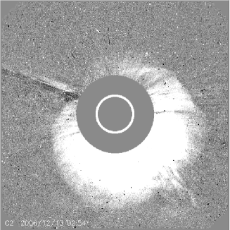
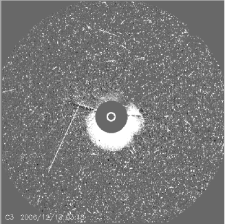
Figure 1: A halo coronal mass ejection observed by the LASCO C2 coronagraph at 02:50 UT (left) and C3 at 03:18 UT (right) on December 13, 2006. These are running difference images where the previous image has been subtracted from the present. The white circle at the center of each image represents the solar surface and the solid grey circle represents the occulting disk. In C3 the so-called “snow storm”, due to high-energy particles striking the LASCO detector, is visible. These later saturate the images in C2 and C3 to the point where no measurements are possible.

By applying well-established assumptions about the observed CME we may identify its distance evolution and mass, from which an estimate of its kinetic and gravitational potential energy may be produced. Distance measurements are obtained by measuring the location of the leading edge of the CME relative to the Sun. Most workers choose a fixed direction or single location on the CME front at which to make these measurements (e.g. Yashiro et al. 2004). Mass is estimated by measuring the intensity across the entire area enclosing the CME and converting it to a density using Thomson scattering theory (e.g. Billings 1966).

Projection effects play an important role in the observed structure of the CME (e.g. Howard and Tappin 2008). LASCO images are projected into the plane of the sky, and so the closer the CME is to the Sun-Earth line, the more heavily projected its images will be. For mass calculations the angle to the plane of the sky is an integral component of the coefficients involved in the Thomson scattering physics (angle $\chi$ in Billings (1966)), and so the direction of propagation can be easily included in the calculations. For identifying 3-D distance properties we may apply spherical geometry provided we have an idea of the direction of propagation of the CME. For the analysis in the present study we apply the technique of Howard et al. (2007, 2008) who used the location of the associated solar surface eruption as the direction of propagation. In this case, this is the flare in AR 10930, which was located at 6^∘S, 23^∘W at the time of the eruption. It is important to note that the location of the flare is not an excellent indicator of CME direction as it has been well established that flares are more usually associated with the footpoint of a CME (e.g. Harrison 1986). In the absence of other 3-D directional information, however, the location of the flare is a reasonable approximator.

Because of these and other uncertainties we consider two values for speed and mass and consequently for the energies: the projected values (unchanged from the original height-time measurements); and de-projected values following the analysis below. These two values may be regarded as lower and upper limits to the calculated values of speed, mass and energy, respectively.

Following Howard et al. (2007) we use the following equation for 3-D distance:

$${1\over{R}}=\sin\alpha\cot\varepsilon+\cos\alpha,$$ (3)

where $R$ is the radial distance of the measured point (on the CME) from the Sun in AU and $\alpha$ is the angle subtended by the measured point at the Sun, given by

$$\cos\alpha=\cos\theta\cos\phi,$$ (4)

where $\theta$ and $\phi$ are the latitude and longitude of the direction of propagation vector, which in this case is the location of the flare site. The angle $\varepsilon$ is the elongation, which is easily obtained via the application of two simple assumptions about CMEs observed by coronagraphs. These are the Point P approximation (e.g. Houminer and Hewish 1972) and that $\varepsilon$ is small. This enables the simple conversion $r$ (AU) = $\varepsilon$ (rad), where $r$ is the projected distance of the measured point (Howard et al. 2007). To determine the mass we use the standard codes for mass calculation available via the Solarsoft software suite (including $eltheory.pro$). These codes are based on the theory of Billings (1966) (page 150) and include the $\chi$ term for direction.

The CME associated with the flare on December 13 was Earth-directed event and first observed by LASCO C2 at 02:54 UT on December 13. Assuming a constant speed its projected onset was 01:49–02:19  UT (de-projected–projected), within the 8 hours between the vector magnetic field measurements. Figure 1 shows LASCO C2 and C3 images of the CME. Shortly after launch, energetic particles from the flare bombarded SOHO resulting in the saturation known as a “snow storm”. The bombardment intensified reaching a point where the LASCO cameras were almost completely saturated by around 04:00 UT. As a result, we were only able to obtain mass measurements from single C2 and C3 images (at 02:54 and 03:18 UT from Figures 1 respectively) and could only obtain height (or distance) – measurement until 04:18 UT.

3 Results

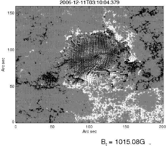
Figure 2: A map of the vector magnetic field of the active region 10930. The transverse field vectors are overlaid upon the B_z component of the magnetic field. The black (white) colors represent the south (north) polarity regions.

The active region NOAA 10930 appeared on the Eastern limb of the Sun on December 5, 2006 in the southern hemisphere at a latitude of 5^∘, with two polarities that were almost perpendicularly aligned with the East-West direction. It was visible on the solar disk until December 17 when it crossed the West limb of the sun (see: http://www.solarmonitor.org/index.php). Figure 2 shows the sample image of the vector magnetogram with the transverse field vectors overlaid upon B_z for the Dec 11 observation. The vertical magnetic field strength in the South (negative) and North (positive) polarity sunspot is in excess of -4000 and 2300 G respectively.

In the vector field map (Figure 2) it is clear that the field lines are twisted. Both the polarities are located close to each other and the boundary between the two is highly sheared. The North polarity region is emerging in the Southern part of the existing South polarity region. As it emerges it rotates in the anti-clockwise direction and the transverse fields are twisted in the clockwise direction.

3.1 Magnetic Energy

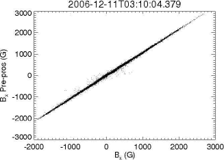
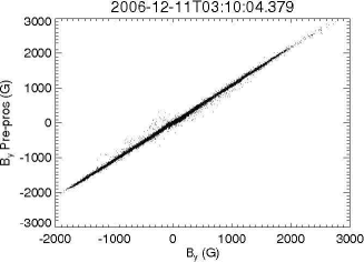
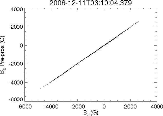
Figure 3: Scatter plots of $B_{x}$(top left), $B_{y}$(top right) and $B_{z}$(bottom) between the photospheric and pre-processed vector field data.

The pre-processed vector magnetograms have been used to compute the magnetic energy. Because of the pre-processing, the 3-components of the magnetic fields have been modified. We compare the pre-processed vector field data with the original data. Figure 3 shows the pixel-by-pixel scatter plot of the same for 3 components of the vector magnetic fields. We have kept the $B_{z}$ component of the magnetic field close to the original as suggested by Metcalf et al. (2008). However, the pre-processing has changed the transverse fields significantly. In order to make sure that the pre-processed vector magnetograms show the force-freeness assumption, we computed the force balance parameter ($\epsilon_{force}$) and torque balance parameter ($\epsilon_{torque}$) as suggested in Wiegelmann, Inhester and Sakurai (2006). We found that the force and torque balance parameters are much smaller than unity. For example, the computed $\epsilon_{force}$ = 0.002 and $\epsilon_{torque}$ = 0.037 for the December 11, pre-processed magnetogram data observed between 03:10 and 04:19 UT. Similarly, the computed $\epsilon_{force}=-0.003$ and $\epsilon_{torque}$ = 0.03 for the December 11, between 08:00 UT and 09:30 UT. This value is much smaller compared to the $\epsilon_{force}$ = 0.17 and $\epsilon_{torque}$ = 0.37 for the original Hinode magnetograms obtained on December 11, between 03:10 and 04:19 UT. A similar value is obtained for the magnetogram taken on December 11, between 08:00 UT and 09:30 UT.

Figure 4: The total magnetic energy ($\star$), the magnetic potential energy ($\diamond$) and the magnetic free energy ($\triangle$) available in the active region is plotted as a function of time. The vertical dashed line represents the onset of the X3.4 class flare.

Figure 4 shows the plot of the total energy ($\star$), magnetic potential energy ($\diamond$) and free magnetic energy ($\triangle$) computed using Equations (1) and (2) as functions of time. The uncertainty in measuring the total magnetic energy involves (1) those from the measurement in the field and (2) those due to the flux imbalance term in the virial theorem. The uncertainty in the magnetic field measurement has been propagated through the magnetic virial energy equation and we have estimated the uncertainty in total magnetic energy. The term $1/8\pi\int_{\delta V}B^{2}(x.n)d^{2}x$ is neglected in the virial energy estimation (see Metcalf et al. 2008). This introduces an uncertainty in the total energy estimation. We estimated the uncertainty introduced by the neglected term in the virial energy by making the assumption that the net flux is spread over the hemisphere uniformly. We have taken the radius of the region of interest as $x$ in the equation and the area as the surface area of the hemisphere. The final uncertainty is $\sqrt{error(1)^{2}+error(2)^{2}}$, where $error(1)$ and $error(2)$ are the uncertainties due to reasons (1) and (2) respectively. The uncertainties obtained from these two are small and shown in the plot. There is one more systematic uncertainty that occurs due to the fact that the field is not force-free in the photosphere. We have used the pre-processing technique to make it more closely approximating the force-free condition. However, there are still residual net forces. These residuals produce a systematic uncertainty in the virial energy estimation. Metcalf et al. (2008) model shows that the net Lorentz force underestimates the virial energy by about 10%. By taking this into account our estimated total virial energy goes up by 10% and hence also the free energy. This systematic underestimation shifts the total energy and free energy curve proportionately to each other. However this does not change the difference in energy between before and after the flare significantly. From the plot it is clear that the free magnetic energy increases with time. However, the increase in the free energy is large on December 11, at 23:10 UT to December 12, at 20:30 UT, and the free magnetic energy accumulated over a period of 20 hrs is estimated to be about 3.7$\times$10³² erg. The last vector magnetogram before the X3.4 class flare was obtained on December 12, at 20:30 UT. The next vector magnetogram was obtained on December 13, at 04:30 UT. So, there is a gap of about 8 hrs between the magnetograms. During this period we observe a decrease in the magnetic free energy of about 3.11$\times$10³² erg. This drop in free energy is clearly seen in the plot after the X3.4 class flare (shown as the dashed vertical line for the onset time of X3.4 class flare) has occurred. Afterwards the free energy again increases with time.

3.2 Energy Carried Away by the Coronal Mass Ejection

In order to compare the available magnetic free energy with the energy carried away by the CME, we have estimated the mechanical energy in the CME. The mass of the CME, averaged between the LASCO C2 and C3 images and assuming both the projected value and that at an angle of 67^∘ from the sky plane, was (8.6–9.3)$\times$10¹⁵ g. Its speed, obtained from a least squares linear fit through the distance-time plot and de-projected using the location of the flare and Equation (3), was 1775–3060 km s^-1. This is a fast and massive CME but not physically unreasonable. CMEs have been known to obtain such speeds early in their evolution but are expected to decelerate rapidly through the heliosphere. Given that the travel time from the Sun to the ACE spacecraft (judging by the arrival of a forward shock at ACE on December 14 around 13:50 UT) was just under $1\frac{1}{2}$ days, such a deceleration was likely. It is noteworthy that following a sudden commencement at 14:15 UT on December 14, a strong geomagnetic storm followed achieving a maximum K${}_{\mbox{p}}$ of 8+ and minimum Dst of –146 nT. Such activity is indicative of the arrival of a large fast CME at the Earth.

The resulting kinetic energy of the CME was therefore (1.35–4.35)$\times$10³² erg. We calculated the gravitational potential energy at each distance from the Sun but it never exceeded 4% of the kinetic energy. Including the gravitational potential energy we estimate the total energy to be (1.4–4.5)$\times$10³² erg. This is (0.45–1.45) times the available magnetic free energy.

3.3 Energy Content of Thermal Plasma

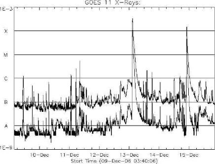
Figure 5: GOES-11 X-ray flux for 5 days starting from Dec 9, 2006. The upper and lower curves in the plot indicates the integrated full-Sun soft X-ray flux in the 1-8 and 0.5-4 Å band passes respectively. The 1-8 Å band pass curves give the X-ray flare index.

Geostationary Operational Environmental Satellite (GOES) provides disk integrated X-ray flux in two wavelength bands, (1) 1-8 Å and (2) 0.5-4 Å (Kahler and Kreplin, 1991). The 1-8 Å bandpass curves give the X-ray flare index. Figure 5 shows the GOES X-ray flux obtained from GOES-11 for the two channels over a period of 7-days around the event of interest. The data from the two channels were used to estimate the radiative soft-X-ray energy. We first subtracted the background flux taken on December 10, 2006 between 19:09 UT and 23:12 UT. Using the solar software pipeline, the temperature of the plasma has been estimated by the taking the ratio of the two channels (Thomas et al. 1985). Using the synthetic solar spectrum, the computed temperature can be converted into an emission measure. By integrating this over the flare duration we obtained the radiated energy by the thermal plasma (integrated between 02:14 UT and 02:54 UT on December 13, 2006). The obtained radiative energy during the flare time is 9.04$\times$10³⁰ erg.

It has already been shown that the ejected CME on Dec 13, 2006 carried a mechanical energy of (1.4–4.5)$\times$10³² erg. The radiative energy loss in the flare plasma is 9.04$\times$10³⁰ erg. Adding the two shows that (1.49–4.59)$\times$10³⁰ erg of energy is utilized. In this energy estimation we do not consider the energy used in the production of SEPs, magnetic field reconfiguration or unerupted plasma transportation.

4 Discussion

The magnetic energy can build up in the process of shearing motion of the magnetic footpoints or during the flux emergence processes. The emerging flux region is the location for many observed solar flares and CMEs (Martin et al. 1982). The emergence of a magnetic field can occur on a small scale (Berlicki et al. 2004) or large scale (Li et al. 2000). In the case of NOAA AR 10930, a large scale magnetic field emerged near the pre existing large south (negative) polarity region. From the magnetic map and transverse vectors it appears that the region between the two polarities is highly sheared (Schrijver et al. 2008). The flux tubes emerge with a twist (Longcope and Welsch 2000) albeit with various quantities. While the twisted flux tube is emerging, it imports magnetic energy and helicity into the corona (Magara and Longcope 2003). In the emerging flux region the energy contribution comes from both the horizontal motion of the footpoint as well as from the vertical motion of emergence. In our study, we do not know how much is the contribution from each of these components. This will be the subject matter of future studies. For the present case, however, our results establish that in an emerging active region such as NOAA 10930 discussed here, the magnetic free energy was increasing until the onset of X3.4 class flare and it accumulated 5.35$\times$10³² erg of magnetic free energy over a period of 4 days.

There have been several studies on this active region to estimate the energy released during the X3.4 class flare on December 13, 2006 based on NLFFF model. Schrijver et al. (2008) have found that there is a drop in energy of 3$\times$10³² ergs during the X3.4 class flare. Guo et al. (2008) have obtained a 2.4$\times$10³¹ ergs of drop in energy after X3.4 class flare. On the other hand Jing et al. (2010) did not find any drop in energy, instead they observed an increase in free energy after the flare. In the present study, we have used a magnetic virial theorem to estimate the magnetic free energy available in the active region. Even though the cadence of the vector field measurement is poor, we were able to see a decrease in the magnetic free energy that persisted even 10 hrs after the flare.

We have identified a reduction of 3.11$\times$10³² erg of magnetic free energy in AR 10930. The CME associated with the energetic event that took place on December 13, 2006 carried about (1.4–4.5)$\times$10³² erg (using projected and deprojected method) of energy. The estimated radiative energy loss during the X3.4 class flare was about 1$\times$10³¹ ergs. The range of energies gives rise to two possibilities: (1) the entire energy for the CME came from the same active region; or (2) only a portion of the CME energy has been supplied by this active region. The latter is based on the assumption that the active region is associated with a single footpoint of the CME (Simnett and Harrison 1984, 1985, Harrison and Simnett 1984, Harrison 1986). If the calculated energy is closer to the projected calculations (the lower limit) then the former is likely true, while if the energy is closer to the de-projected values then the latter applies.

The latter possibility is more likely for this event given that it is a halo CME and therefore likely to be highly projected in the LASCO images. Let us consider the upper extreme of the energy. Half of the CME energy is around 2.25$\times$10³² erg, which leaves 8.6$\times$10³¹ erg in the lost magnetic free energy available for other purposes. Emslie et al. (2004) determined the energy budget on two flare/CME events on 21 April and 23 July 2002. Both were associated with an X-class flare (X1.5 for the former and X4.8 for the latter). They found that the flares contributed between 1-4$\times$10³¹ erg, which included the energy for particle acceleration. Given that flares are broadband phenomena the emission energy contribution extends across the electromagnetic spectrum, and so a larger energy budget for emission is expected. We must also consider the energy in moving around solar plasma and un-erupted magnetic fields (e.g. Webb et al. 1980). It is not unreasonable to conclude that this energy budget combined could accommodate the remaining magnetic energy ($\sim$8.6$\times$10³¹ erg) that did not contribute to the CME.

At this stage, however, we do not have sufficient evidence to determine which possibility is correct, but it is noteworthy that the calculated energy range (for the CME) includes the value for the available free energy, which lies almost exactly halfway (by ratio) between the two extremes.

The actual magnetic free energy release could also be larger than that computed. This is because of the following reasons:

1. The magnetic flux was still emerging before the flare (Park et al. 2010) and our preflare magnetic field measurement was about 5 hrs before the flare. So, the available free energy could be larger than estimated here.

2. The post-flare energy calculation was performed at a time one hour after the post-flare time. Within this 1 hr gap the free energy would have increased as the flux was still increasing (Park et al. 2010). Hence the measured dip in free energy could be larger.

3. The photosphere is not force-free. To make it close to the force-free we have used the pre-processing technique that may reduce the actual value of the available energy. Metcalf et al. (2008) have applied a realistic model to test the Lorentz forces in the photosphere. In their model they compared the net force at various heights. They have found that the net force falls close to zero at the chromospheric height but not in the photosphere. Due to this net force at the photospheric level there is an underestimation of the virial energy by about 10%. Hence, the free energy will also be underestimated by the same amount. However, this underestimation will not affect significantly the change in free magnetic energy measurement between before and after the flare.

4. It is not well known how much the 180^∘ ambiguity will affect the virial energy estimation.

We have identified the source of uncertainty in the energy estimation using the virial theorem. The estimated uncertainty is much smaller than the free energy. Metcalf, Leka and Mickey (2005) have estimated the uncertainty in magnetic energy estimation by pseudo-Monte Carlo method by displacing the origin to different locations on the vector fields. This method is valid only if the measured field is forced. However, the pre-processing technique makes these fields close to force-free and hence measuring the mean value of the energy by shifting the origin to different locations on the image is not required. Wheatland and Metcalf (2006) have introduced a new method to find the magnetic energy using the virial theorem. However, that method depends on the choice of the model to compute the vertical field gradients. In the absence of chromospheric magnetic field measurements they have used the linear force-free parameter ($\alpha$) to compute the vertical field gradients. The distribution of magnetic field deviates from the constant $\alpha$ in most of the locations in the active region. Hence, a detailed study is required to find further details on how this method is superior to the other methods. Until then the method of using the pre-processed data for the virial energy estimation is a better choice than those methods.

The largest source of error in the CME calculations is the 3-D information provided for the de-projection. We used the location of the flare to provide values for $\theta$, $\phi$ (distance) and $\chi$ (mass) but this assumption is limited. Firstly, it is not appropriate to assume that the CME originated from the flare or even the active region, and secondly the CME cannot be regarded as a point source (as assumed for the distance measurements). The CME is a large structure and for the larger ones the associated flare and active region are typically associated with a single footpoint only. In this case, 3-D assumptions based on the flare and AR would provide information on just that footpoint. This is also the reason why we assume for the maximum case that only half of the CME’s energy was provided by the AR. To our knowledge no systematic empirical study of the source of energy for the CME has yet been conducted so it is unknown what proportion of its energy budget arises from the AR. Given the values we arrived at from the present study, however limited, it seems that a 50% contribution may be a reasonable first-order assumption. Such knowledge may lead to a greater understanding of the onset mechanism for CMEs.

Jing et al. (2009) have observed for many active regions that there is a decrease in magnetic free energy 15 min before the peak time of the associated non-thermal flare emission. Such studies cannot be taken up with the present data as the cadence of vector magnetic field measurement is poor. The Solar Dynamic Observatory (SDO) (launched February 2010) provides vector field measurements at high cadence. Hence, the SDO data set may provide a complete picture on how the free energy changes close to the flare time and during the flare. However, for a better estimation of the available free energy we need to have chromospheric vector magnetic field data (Metcalf, et al. 2005). Currently, the chromospheric vector field data are not available on regular basis. Until they are available, photospheric vector magnetogram with the pre-processing techniques will provide the good boundary data for estimating the magnetic free energy.

5 Conclusions

Solar flares and CMEs are responsible for the release of large amounts of energy from the Sun. During solar flares energy is redistributed partly in the form of broadband emission from X-rays to the radio band. The energy is also carried by the thermal plasma, accelerated electrons, etc. The vast majority of the energy budget, however, is allocated to mechanical energy in the form of an expanding CME.

Using the high resolution time sequence of vector magnetograms from SOT/SP we studied the temporal evolution of magnetic free energy in an active region NOAA 10930. We then compared the available magnetic free energy with the energy carried away by the halo CME. From the analysis we arrive at the following conclusions:

1. The free magnetic energy increases with time and about 3.7$\times$10³² erg of magnetic free energy is accumulated over a period of about 20 hrs before the X3.4 class flare and CME launch occurred.

2. There is a decrease in magnetic free energy of about 3.11$\times$10³² erg during the flare/CME.

3. The estimated energy carried away by the CME is (1.4–4.5)_×10³² ergs (using projected and de-projected values). This is 0.5–1.5 times larger than the estimated magnetic free energy.

4. The estimated radiative energy loss during the X3.4 class flare is 9.04$\times$10³⁰ erg.

   We believe that more energy was carried by the CME than was available in the active region, as some of the free energy must be allocated to radiative energy loss, particle acceleration and plasma and magnetic field reorientation. Given the range of energies calculated for CME and the possibility that the free magnetic energy may be larger, one could easily conclude that the entire energy was provided by the active region.

References

- [1] Alissandrakis, C. E. 1981, A&A, 100, 197
- [2] Aly, J. J. 1984, ApJ, 283, 349.
- [3] Berlicki, A., Schmieder, B., Vilmer, N., Aulanier, G. and Del Zanna, G., 2004, A&A 423, 1119.
- [4] Billings, D.E., 1966, A Guide to the Solar Corona, Academic Press, New York.
- [5] Brueckner, G. E., Howard, R. A., Koomen, M. J., Korendyke, C. M., Michels, D. J., Moses, J. D., Socker, D. G., Dere, K. P., Lamy, P. L., Llebaria, A., Bout, M. V., Schwenn, R., Simnett, G. M., Bedford, D. K., and Eyles, C. J., 1995, Solar Phys., 162, 357.
- [6] Canfield, R. C., Cheng, C.-C., Dere, K. P., Dulk, G. A., McLean, D. J., Robinson, Jr., R. D., Schmahl, E. J., and Schoolman, S. A., 1980, in Solar Flares: A Monograph From Skylab Workshop II, Sturrock, P. A (ed.), Colo. Assoc. Uni. Press, Boulder Colo, 451.
- [7] Chandrasekhar, S. 1961, Hydrodynamic and Hydromagnetic Stability (NewYork:Dover).
- [8] De Rosa, M. L., Schrijver, C. J.; Barnes, G. Leka, K. D., Lites, B. W. and Aschwanden, M. J., et al. 2009, ApJ, 696, 1780.
- [9] Emslie, A. G., Kucharek, H., Dennis, B. R., Gopalswamy, N., Holman, G. D., Share, G. H., et al. 2004, JGR, 109, A10104.
- [10] Gary, G. A., Moore, R. L., Hagyard, M. J., and Haisch, B. M., 1987, 314, 782.
- [11] Gary, G. A., 1989, ApJS, 69, 323.
- [12] Guo, Y. Ding, M. D., Wiegelmann, T., and Li H., 2008, ApJ, 679, 1629.
- [13] Harrison, R. A., 1986, A&A, 162, 283.
- [14] Harrison, R. A., Simnett, G.M., 1984, Adv. Space Res. 4, 199.
- [15] Howard, T. A., Fry, C. D., Johnston, J. C., and Webb, D. F., 2007, ApJ, 667, 610.
- [16] Howard, T. A., Nandy, D., and Koepke, A. C., 2008, JGR, A01104, doi:10.1029/2007JA012500.
- [17] Howard, T. A., and Tappin, S. J., 2008, Solar Phys., 252, 373.
- [18] Houminer, Z., and Hewish, A., 1972, Planet. Space Sci., 20, 1073.
- [19] Ichimoto, K., Lites, B., Elmore, D., Suematsu, Y., Tsuneta, S., et al. 2008, Solar Phys. 249, 233.
- [20] Isobe, H., et al. 2007, PASJ, 59, 807
- [21] Jing, Ju, Chen, P. F., Wiegelmann, T., Xu, Y., Park, S. H., and Wang, H., 2009, ApJ 696, 84.
- [22] Jing, Ju, Yuan, Y. Wang, B., Wiegelmann, T., Xu, Y. and Wang, H. 2010, ApJ, 713, 440.
- [23] Kahler, S. W., and Kreplin, R. W., 1991, SoPh, 133, 371.
- [24] Kazachenko, M. D., Canfield, R. C., Longcope, D. W., Qiu, J., Des Jardins, A. and Nightingale, R. W., 2009, ApJ, 704, 1146.
- [25] Kosugi, T., Matsuzaki, K., Sakao, T. et al. 2007, Solar Phys., 243, 3.
- [26] Leka, K. D., Barnes, G., and Crouch, A. D. 2009, In Second Hinode Science Meeting, ASP Conference Series, 416, 127.
- [27] Li, H., Sakurai, T. Ichimoto, K. and UeNo, S., 2000, PASJ, 52, 483.
- [28] Lin, H., Kuhn, J. R. and Coulter, R., 2004, ApJ, 613, 177.
- [29] Lites, B. W. and Skumanich, A. 1990, ApJ, 348, 747.
- [30] Lites, B. W., Elmore, D. F., Seagraves, P., and Skumanich, A. P., 1993, ApJ, 418, 928.
- [31] Longcope, D. W. and Welsch, B. T., 2000, ApJ, 545, 1089.
- [32] Longcope, D. W., Beveridge, C., Qiu, J., Ravindra, B., Barnes, G., and Dasso, S., 2007, Solar Phys., 244, 45.
- [33] Low, B. C., 1985 in Measurement of Solar Vector Magnetic Fields, ed. M. J. Hagyard (NASA Conf. Pub. 2374), 49.
- [34] Magara, T. and Longcope, D. W., 2003, ApJ, 586, 630.
- [35] Magara, T., and Tsuneta, S. 2008, PASJ, 60, 1181.
- [36] Martin, S. F., Dezso, L., Antalova, A., Kucera, A. and Harvey, K. L. 1982, AdSR, 2, 39.
- [37] Metcalf, T., 1994, Solar Phys., 155, 235.
- [38] Metcalf, T. R., Jiao, L, McClymont, A, N.; Canfield, R, C. and Uitenbroek, H., 1995, ApJ, 439, 474.
- [39] Metcalf, T. R., Leka, K. D. and Mickey, D. L., 2005, ApJ, 623, 53.
- [40] Metcalf, T. R., De Rosa, M. L., Schrijver, C. J., Barnes, G. et al., 2008, Solar Phys., 247, 269.
- [41] Min, S. and Chae, J., 2009, Solar Phys., 258, 203.
- [42] Molodenskii, M. M., 1969, SVA, 12, 585.
- [43] Park, S. H., Chae, J., Jing, Ju, Tan, C., and Wang, H., 2010, ApJ, 720, 1102.
- [44] Ravindra, B., Longcope, D. W. and Abbett, W. P., 2008, ApJ, 677, 751.
- [45] Sakurai, T., 1987, Solar Phys., 113, 137.
- [46] Schrijver, C. J., De Rosa, M. L., Metcalf, T., Barnes, G., Lites, B., Tarbell, T., McTiernan, J., Valori, G., Wiegelmann, T., Wheatland, M. S., et al., 2008, ApJ, 675, 1637.
- [47] Skumanich, A., and Lites, B. W. 1987, ApJ, 322, 473.
- [48] Simnett, G. M., Harrison, R. A., 1984, Adv. Space Res., 4, 279.
- [49] Simnett, G. M., Harrison, R. A., 1985, Solar Phys. 99, 291.
- [50] Solanki, S. K., Lagg, A., Woch, J., Krupp, N. and Collados, M., 2003, Nature, 425, 692.
- [51] Srivastava, N., Mathew, S. K., Rohan, L. E., Wiegelmann, T., 2009, JGRA, 11403107.
- [52] Su, J. T., Sakurai, T., Suematsu, Y., Hagino, M. and Liu, Yu, 2009, ApJ, 697, 103.
- [53] Tan, C., Chen, P. F., Abramenko, V., and Wang, H. 2009, ApJ, 690, 1820.
- [54] Thosmas, R. J., Crannell, C. J., and Starr, R., 1985, Solar Phys. 95, 323.
- [55] Venkatakrishnan, P., Hagyard, M. J., and Hathaway, D. H. 1988, Solar Phys., 115, 125.
- [56] Venkatakrishnan, P and Ravindra, B., 2003, GRL, 30, 2181.
- [57] Webb, D. F., Cheng, C.-C., Dulk, G. A., Edberg, S. J., Martin, S. F., McKenna-Lawlor, S., and McLean, D. J., 1980, in Solar Flares: A Monograph From Skylab Workshop II, Sturrock, P. A (ed.), Colo. Assoc. Uni. Press, Boulder Colo, 471.
- [58] Wheatland, M. S., and Metcalf, T. R., 2006, ApJ, 636, 1151.
- [59] Wiegelmann, T., Inhester, B., and Sakurai, T., 2006, Solar Phys., 233, 215.
- [60] Wiegelmann, T., Thalmann, J. K., Schrijver, C. J., De Rosa, M. L., and Metcalf, T. R., 2008, Solar Phys., 247, 249.
- [61] Yashiro, S., Gopalswamy, N., Michalek, G., St. Cyr, O. C., Plunckett S. P., and Howard, R. A., 2004, JGR, 109, doi:10.1029/2003JA010282.