Solar system constraints on asymptotically flat IR modified Ho$\check{r}$ava gravity through light deflection

Abstract

In this paper, we study the motion of photons around a Kehagias-Sfetsos (KS) black hole and obtain constraints on IR modified Ho$\check{r}$ava gravity without cosmological constant ($\sim\Lambda_{W}$). An analytic formula for the light deflection angle is obtained. For a propagating photon, the deflection angle $\delta\varphi$ increases with large values of the Ho$\check{r}$ava gravity parameter $\omega$. Under the UV limit $\omega\longrightarrow\infty$, deflection angle reduces to the result of usual Schwarzschild case, $4GM/R$. It is also found that with increasing scale of astronomical observation system the Ho$\check{r}$ava-Lifshitz gravity should satisfy $|\omega M^{2}|>1.1725\times 10^{-16}$ with $12\%$ precision for Earth system, $|\omega M^{2}|>8.27649\times 10^{-17}$ with $17\%$ precision for Jupiter system and $|\omega M^{2}|>8.27650\times 10^{-15}$ with $0.17\%$ precision for solar system.

I Introduction

It is known that the Lagrangian of original Lifshitz scalar field theory is

$$\mathcal{L}=\int d^{2}xdt\left[\left(\partial_{t}\phi\right)^{2}-\lambda_{L}\left(\Delta^{2}\phi\right)^{2}\right],$$ (1)

which has a line of fixed points parameterized by $\lambda_{L}$ with anisotropic scale invariance Lifshitz . So such fixed points are the so-called Lifshitz points. Recently, Ho$\check{r}$ava adopted one Lifshitz scale in time and space, and obtained a renormalizable gravity theory at these Lifshitz point Horava1 ; Horava2 ; Horava3 . It is known also as Ho$\check{r}$ava-Lifshitz (HL) gravity. It exhibits a broken Lorentz symmetry at the short distances, but it reduces to usual General Relativity (GR) at the large distances due to these non-contribution of higher derivative terms with particular $\lambda=1$. The parameter $\lambda$ controls the contribution of the extrinsic curvature trace. However, it is possible that HL at large distance could deviate from GR for the incomplete diffeomorphism invariance. In this paper, we only consider the simple case of $\lambda=1$. Since HL gravity theory was put forth, HL gravity is intensively investigated in many aspects. They are developments of basic formalism Sotitiou ; Visser ; CCai ; Chenen ; Orlando ; CCCai ; Nishioka1122 ; LiLIli ; Charmousis ; Sotiriou111 ; calagni222 ; Blas333 ; Iengo ; Germani11 ; Mukohyama1 ; Appignani1 ; Kluson1 ; Afshordi ; Kobakhidze1 ; Kobakhidze2 , cosmology Kiritsis ; Mukohyama ; Brandenberger ; Piao ; Mukohyama2 ; Kalyana2 ; chen1 ; Wang1 ; Nojiri ; Cai1 ; Wang2 ; Kobayashi1 , dark energy and dark matter Saridakis ; Park ; Mukohyama11 , various black hole solutions and their thermodynamics Saridakis ; Park ; Mukohyama11 ; Nastase ; Cai22 ; Myung ; Cai33 ; Mann ; Bottacant ; Castillo ; Peng111 ; Colgain ; Lee ; Kim111 ; Park22 ; Lu ; Kehagias ; Koutsoumbas1 ; Koutsoumbas2 ; Majhi222 and so on.

With the subsequent developments of the HL gravity, the following problem raised in front of us: how does the matter fields influence the geometry? Several researchers made efforts to find the analogue of the matter energy-momentum tensor acting gravitational source as GR. The study of its geodesic in HL theory is the first step for finding a solution. Hence, some pioneering works addressed this aspect with various methods. They are the optical limit of a scalar field theory Capasso , super Hamiltonian formalism Rama , foliation preserving diffeomorphisms Mosaffa , Lorentz-violating Modified Dispersion Relations Sindoni as well as observational kinematic constraints below mentioned chenjuhua ; Iorio1 ; Iorio2 ; Harko11 . In particular, in the framework of the optical limit Capasso and Polychronakos Capasso gave us a comprehensive study of particles in the HL gravity. Based on the optical limit, the deformed geodesic equation was derived from a generalized Klein-Gordon action. Such results clearly show that the fact that the particles move along geodesic, which depend on the mass of particles, is not granted. Deviations from geodesic motion appear both in flat and Schwarzschild-like spacetimes. This type deformed kinematics could allow the presence of superluminal particle for particular $\lambda$ ( or $\tilde{\lambda}$’s in Ref.Capasso ) which could not give any restriction on the velocity. The particles with given $\tilde{\lambda}$’s could be always accelerated to any velocity under an action of constant force. Else, the higher is the energy of the particle, the larger will be the deviation from the geodesic motion determined by the low-energy four dimensional metric $g_{\mu\nu}$. Similar results deviations from GR also are found in Rama ; Mosaffa ; Sindoni with various above-mentioned approaches.

On the other hand, a specific case of asymptotically flat IR modified HL gravity under the cosmological constant limit $\Lambda_{W}\longrightarrow 0$ in HL gravity is proposed by Kehagias and Sfetsos Kehagias . It reduces to GR gravity in IR regime according to coupling $\lambda$.The massless excitation with two propagating polarizations emerges in the Minkowski vacuum, which is admitted naturally, with the transverse traceless part of the perturbation. At the most important, one static spherically symmetric black hole solution of HL gravity i.e. KS black hole is obtained, which can be treated as counterpart of the Schwarzschild case in GR. Comparing its geometry with GR, it is also found that this solution has the same Newtonian and post-Newtonian limits which ensures its soundness when it is confronted with the astronomical observational data. Since then, there are some works involving the phenomenology of the deformed HL black hole, such as strong field gravitational lensing chensongbai1 ; Konoplya , black hole’s quasi-normal modes Konoplya ; chensongbai2 , timelike Geodesic Motion chenjuhua , thin accretion disk Harko1 . In Konoplya’s work Konoplya , the gravitational lensing and quasi-normal modes are considered, which are potentially observable properties of black holes beyond the post-Newtonian corrections. It is found that the bending angle is smaller and the real oscillation frequency of quasinormal modes (QNM) is larger than that of GR case. The QNM can be lived longer in this deformed HL black hole. In Chen’s work chensongbai1 , the angular position and magnification of the relativistic images are obtained with strong field gravitational lensing. Unlike the former Konoplya’s work Konoplya , a scheme to distinguish a deformed HL black hole from a Reissner-Norstr$\ddot{o}$m black hole is introduced. Comparing with the latter work, the angular position decreases more slowly with bigger HL gravity parameter $\omega$. Else, angular separation increases more rapidly. In Chen’s another work chensongbai2 , it is also found that the scalar perturbations decay more slowly in the HL gravity. In Ref. chenjuhua , the time-like geodesic motion is analyzed with the effective potential in this deformed HL gravity. In Harko’s work Harko1 , by using the accretion disk properties, one can obtain some important properties such as the energy flux, the temperature distribution, the emission spectrum and so on. Unlike the usual GR, there are some particular signatures appeared in the electromagnetic spectrum which maybe supply a observable path for HL gravity.

With the development of KS black hole, there are some works referring to field parameters constraints such as the solar system orbital motions Iorio1 , the extrasolar planets and double pulsar Iorio2 , the solar system three classical tests Harko11 and so on. In Iorio1 ; Iorio2 lower bounds on $\omega$ are obtained via the post-Newtonian motion equation.

As we know that, the asymptotically flat HL gravity with $\lambda=1$ reduces to the Schwarzschild space with the limit of $\omega\longrightarrow+\infty$. So in the UV limit, the field parameter $\omega$ should be large enough to ensure the UV Ho$\check{r}$ava gravity is in conformity with GR gravity well. Motivated by above various factors, one aim of this paper is to find the lower limit of HL gravity field parameter $\omega$. Considering the last work Harko11 , the numerical constraints results are obtained directly from integrating metric function by using the static and spherically symmetric metric. Hence, another aim of this paper is to find the analytic expression of light deflection. We adopt one approach of Lagrange analysis and study the light deflection in the KS black hole in HL gravity under the weak field and the slow motion approximation. Then, we also compare our results with the observational data (long baseline radio interferometry, Jupiter measurement, Hipparcos satellite) and we also obtain corresponding constraints on HL field parameter $\omega$ for solar system, Jovian planet system and Earth system, respectively.

This paper is organized as follows. In section II, we present the action of HL gravity and spherically symmetric Kehagias and Sfetsos black hole. In section III, we calculate the general solution to motion equation of photons in deformed HL gravity. In section IV, we use astronomical observations to constrain the HL gravity. In Section V we compare our results with other constraints obtained from inside and outside solar system. Section VI is devoted to the conclusions. We adopt the signature $(-,+,+,+)$ and put $\hbar$, $c$, and $G$ equal to unity.

II The asymptotically flat black hole solution in the deformed HL gravity

In this section, we review briefly the KS black hole solutions under the limit of $\Lambda_{W}\longrightarrow 0$ with running constant $\lambda=1$ in the IR critical point $z=1$. The spacetime geometry is, in the ADM formalism ADD ,

$$ds^{2}=-N^{2}dt^{2}+g_{ij}\left(dx^{i}+N^{i}dt\right)\left(dx^{j}+N^{j}dt\right),$$ (2)

where the classical scaling dimensions of the field are

$$[g_{ij}]_{s}=0,\ \ [N]_{s}=0,\ \ [N^{i}]_{s}=2.$$ (3)

The action for the fields of HL theory is

$$S = \int dtd^{3}x\sqrt{g}N\bigg{\{}\frac{2}{\kappa^{2}}\left(K_{ij}K^{ij}-\lambda K^{2}\right)-\frac{\kappa^{2}}{2w^{4}}C_{ij}C^{ij}+\frac{\kappa^{2}\mu}{2w^{2}}\epsilon^{ijk}R_{il}^{(3)}\nabla_{j}R^{(3)l}_{\ \ \ \ k}$$ (4)

$$\ \ \ \ \ \ \ \ \ \ \ \ \ \ \ \ \ \ \ -\frac{\kappa^{2}\mu^{2}}{8}R_{ij}^{(3)}R^{(3)ij}+\frac{\kappa^{2}\mu^{2}}{8\left(1-3\lambda\right)}\left(\frac{1-4\lambda}{4}\left(R^{(3)}\right)^{2}+\Lambda_{W}R^{(3)}-3\Lambda^{2}_{W}\right)+\mu^{4}R^{(3)}\bigg{\}},$$

where the second fundamental form, extrinsic curvature $K_{ij}$, and the Cotton tensor $C^{ij}$ are given as follows,

$$K_{ij} = \frac{1}{2N}\left(\frac{\partial}{\partial t}g_{ij}-\nabla_{i}N_{j}-\nabla_{j}N^{i}\right),$$ (5)

$$C^{ij} = \epsilon^{ikl}\nabla_{k}\left(R^{(3)j}_{l}-\frac{1}{4}R^{(3)}\delta_{l}^{j}\right).$$ (6)

Here, $\kappa$, $\lambda$, $w$ are dimensionless coupling constants and $\mu$, $\Lambda_{W}$ are dimensional parameters having dimensions of masses $[\mu]=1$, $[\Lambda_{w}]=2$. The last term of metric (4) represents a soft violation of the detailed balance condition. In the limit of $\Lambda_{W}\longrightarrow 0$, we can obtain a deformed action as follows,

$$S = \int dtd^{3}x\left(\mathcal{L}_{0}+\mathcal{L}_{1}\right),$$ (7)

$$\mathcal{L}_{0} = \sqrt{g}N\bigg{\{}\frac{2}{\kappa^{2}}\left(K_{ij}K^{ij}-\lambda K^{2}\right)\bigg{\}},$$ (8)

$$\mathcal{L}_{1} = \sqrt{g}N\bigg{\{}\frac{\kappa^{2}\mu^{2}\left(1-4\lambda\right)}{32\left(1-3\lambda\right)}\mathcal{R}^{2}-\frac{\kappa^{2}}{2w^{4}}\left(C_{ij}-\frac{\mu w^{2}}{2}R_{ij}\right)\left(C^{ij}-\frac{\mu w^{2}}{2}R^{ij}\right)+\mu^{4}\mathcal{R}\bigg{\}}.$$ (9)

Comparing these with the usual GR ADM formalism, we can obtain the speed of light $c$, the Newton’s constant $G$ and the cosmological constant $\Lambda$

$$c=\frac{\kappa^{2}\mu}{4}\sqrt{\frac{\Lambda_{W}}{1-3\lambda}},\ \ G=\frac{\kappa^{2}}{32\pi c},\ \ \Lambda=\frac{3}{2}\Lambda_{W}.$$ (10)

For the particular case of $\lambda=1$ with $\omega=16\mu^{2}/\kappa^{2}$, a spherically symmetric black hole solution is presented by Kehagias and Sfetsos Kehagias , which also is corresponding to an asymptotically flat space,

$$ds^{2}=-f(r)dt^{2}+\frac{dr^{2}}{f(r)}+r^{2}\left(d\theta^{2}+\sin^{2}\theta d\varphi^{2}\right).$$ (11)

The lapse function is

$$f(r)=1+\omega r^{2}-\sqrt{r\left(\omega^{2}r^{3}+4\omega M\right)},$$ (12)

where the parameter $M$ is an integration constant with dimension $[M]=-1$. Using the null hypersurface condition, one can find there are two horizons, inner $r_{-}$ and outer event horizon $r_{+}$ in this space,

$$r_{\pm}=M\left(1\pm\sqrt{1-\frac{1}{2\omega M^{2}}}\right).$$ (13)

The Hawking temperature is

$$T_{H}=\frac{\sqrt{2M^{2}\omega-1}}{\pi\sqrt{2\omega}(r_{+}^{2}+\frac{1}{\omega}+\sqrt{r_{+}^{4}+4\frac{Mr_{+}}{\omega}})}.$$ (14)

The corresponding black hole thermodynamics and its generalized uncertainty principle are studied in Ref. Myungadda . It is also found that if $r\gg(M/\omega)^{1/3}$, this KS solutions will reduce to usual Schwarzschild case and the lapse function can be rewritten as

$$f\approx 1-\frac{2M}{r}+\mathcal{O}(r^{-4}).$$ (15)

Apparently, the former integration constant $M$ is the real mass of black hole.

III motion of photons in HL gravity: general solution

By using the lapse function of KS black hole (11), the usual Lagrangian of test particle is given as

$$2\mathcal{L}_{p}=-f(r)\dot{t}^{2}+\frac{\dot{r}^{2}}{f(r)}+r^{2}\left(\dot{\theta}^{2}+\sin^{2}\theta\dot{\varphi}^{2}\right),$$ (16)

where the overdot represents differentiation with respect to the affine parameter $\xi$ along the geodesics. The Euler-Lagrange equations below give us the kinetic equation of photons,

$$\frac{d}{d\xi}\left(\frac{\partial\mathcal{L}_{p}}{\partial\dot{x}^{\mu}}\right)-\frac{\partial\mathcal{L}_{p}}{\partial x^{\mu}}=0.$$ (17)

Without loss of generality, it is assumed that the observer is confined to orbits with $\theta=\pi/2$ and $\dot{\theta}=0$. Hence, the Lagrangian $\mathcal{L}_{p}$ reduce to

$$2\mathcal{L}_{p}=-f(r)\dot{t}^{2}+\frac{\dot{r}^{2}}{f(r)}+r^{2}\dot{\varphi}^{2}.$$ (18)

According to the Euler-Lagrange equations (17) and reduced Lagrangian $\mathcal{L}_{p}$ (18), we can identify two constant motions for cyclic coordinates $\varphi$ and $t$,

$$f(r)\dot{t} = E,$$ (19)

$$r^{2}\dot{\varphi} = L,$$ (20)

where $E$ and $L$ are the linear momentum and angular momentum at infinite distance. According to the condition for photons $g_{\mu\nu}p^{\mu}p^{\nu}=0$ where $p^{\mu}\equiv\frac{dx^{\mu}}{d\xi}=\dot{x}^{\mu}$ is the photons momentum, we can obtain a relation of parameters ($\dot{t},\dot{r},\dot{\varphi}$) as,

$$-f(r)\dot{t}^{2}+\frac{1}{f(r)}\dot{r}^{2}+r^{2}\dot{\varphi}^{2}=0.$$ (21)

Dividing Eq. (21) by $\dot{\varphi}^{2}$, we can obtain motion equation as

$$-f(r)\left(\frac{\partial t}{\partial\varphi}\right)^{2}+\frac{1}{f(r)}\left(\frac{\partial r}{\partial\varphi}\right)^{2}+r^{2}=0.$$ (22)

Substituting Eqs.(19), (20) into Eq. (22), we can obtain the final photons’ orbital equation

$$\left(\frac{1}{r^{2}}\frac{dr}{d\varphi}\right)^{2}=\frac{1}{b^{2}}-\frac{1}{B^{2}(r)},$$ (23)

where $E$ and $L$ are coupled via $b=L/E$ which represents the effective sighting range or impact parameter. The corresponding photon effective potential $1/B^{2}(r)$ is given as

$$B^{2}(r)=\frac{r^{2}}{1+\omega r^{2}-\sqrt{r\left(\omega^{2}r^{3}+4\omega M\right)}}.$$ (24)

Fig.(1) clearly illustrates that the potential becomes smaller for a larger $\omega$. One also could find that with the bigger HL gravity parameter $\omega$ the curves tends toward the usual GR Schwarzschild result which is drew with bigger red dotted line in Fig.(1). This phenomenon is in agreement with the Schwarzschild limit $r^{3}\gg M/\omega$ Kehagias , in which for the fixed variables $r$ and the central mass parameter $M$, the rewritten Schwarzschild limit is $\omega\gg M/r^{3}$. Hence, the bigger $\omega$ will lead to a final Schwarzschild case.

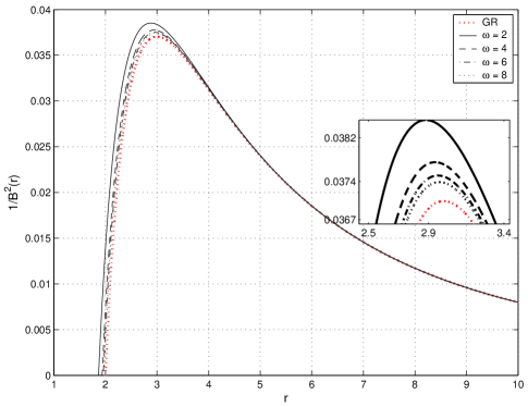
Figure 1: The effective potentials $1/B^{2}(r)$ of photons with unit mass and various parameters $\omega$. The usual Schwarzschild case in GR is denoted with bigger dotted red line.

The constant impact parameter $b$ in Eq. (23) can be eliminated via calculating the derivation with respect to $\varphi$. So the photon Binet equation can be obtained

$$\frac{d^{2}u}{d\varphi^{2}}=-u+3u^{2}\sqrt{\omega M^{2}}\left(\omega M^{2}+4u^{3}\right)^{-\frac{1}{2}},$$ (25)

where $u=M/r$. Considering the fact of that all astronomical observations can be explained very well by the Schwarzschild gravity in solar system, we adopt the Schwarzschild approximation $r\gg(M/\omega)^{1/3}$. Hence, the final general solution to photon orbital equation (23) is written directly as

$$u=u_{0}\cos\varphi+u_{0}^{2}\left(1+\sin^{2}\varphi\right)+\frac{a}{2}\left(\varphi\sin\varphi-\frac{1}{8}\cos 3\varphi-\frac{1}{120}\cos 5\varphi\right).$$ (26)

Here, the parameters $u_{0}$ and $a$ are $u_{0}=GM/R$ and $a=-15u_{0}^{5}/4\omega M^{2}$ where $R$ is the solar radius and $M$ is the solar mass. In the right hand side of Eq. (26), the first term $u_{0}\cos\varphi$ is a straight line normal to pole axis without considering the influence of gravity, the second term $u_{0}^{2}\left(1+\sin^{2}\varphi\right)$ is the standard form coming from general relativity gravity, and the last one $\frac{a}{2}\left(\varphi\sin\varphi-\frac{1}{8}\cos 3\varphi-\frac{1}{120}\cos 5\varphi\right)$ is an improvement of HL Gravity. Part of some related calculations are given in the following section.

IV Solution to photon orbital equation with Ho$\breve{r}$ava-Lifshitz Gravity

Under Schwarzschild approximation $r\gg(M/\omega)^{1/3}$, the photon Binet equation Eq.(25) reduces to a solvable form,

$$\frac{d^{2}u}{d\varphi^{2}}=-u+3u^{2}-6\frac{u^{5}}{\omega M^{2}}.$$ (27)

Considering the small $u$, the high-order small quantities $u^{2}$ and $u^{5}$ can be ignored firstly. So we can obtain the zeroth-order approximate solution

$$u=u_{0}\cos\varphi,$$ (28)

where parameter $u_{0}=GM/R$ is a constant about solar system. Mathematically, this solution is a straight line normal to the pole axis. In order to simplify the calculation, we only replace the high-order terms with the zeroth-order solution in Eq. (27) not the fussy iteration step by step. Hence, one can get

$$\frac{d^{2}u}{d\varphi^{2}}=-u+3u_{0}^{2}\cos^{2}\varphi-\frac{6u_{0}^{5}}{\omega M^{2}}\cos^{5}\varphi.$$ (29)

After decreasing the powers of $\cos^{5}\varphi$ term, Eq.(29) can be reduced a new form

$$\frac{d^{2}u}{d\varphi^{2}}+u=3u_{0}^{2}\cos^{2}\varphi-\frac{3u_{0}^{5}}{8\omega M^{2}}\cos 5\varphi-\frac{15u_{0}^{5}}{8\omega M^{2}}\cos 3\varphi-\frac{15u_{0}^{5}}{4\omega M^{2}}\cos\varphi.$$ (30)

Because the right hand of Eq.(30) includes four terms, we can decompose this ordinary differential equation (30) into corresponding four sub-equations to solve. Here, we list these particular solutions in the Table 1.

Table 1: The particular solutions to Eq.(30).

Sub-equation	Particular solution
$\frac{d^{2}u}{d\varphi^{2}}+u=3u_{0}^{2}\cos^{2}\varphi$	$u=u_{0}^{2}\left(1+\sin^{2}\varphi\right)$
$\frac{d^{2}u}{d\varphi^{2}}+u=-\frac{3u_{0}^{5}}{8\omega M^{2}}\cos 5\varphi$	$u=-\frac{a}{240}\cos 5\varphi$
$\frac{d^{2}u}{d\varphi^{2}}+u=-\frac{15u_{0}^{5}}{8\omega M^{2}}\cos 3\varphi$	$u=-\frac{a}{16}\cos 3\varphi$
$\frac{d^{2}u}{d\varphi^{2}}+u=-\frac{15u_{0}^{5}}{4\omega M^{2}}\cos\varphi$	$u=\frac{a}{2}\varphi\sin\varphi$

Hence, the total particular solution is

$$u^{*}=u_{0}^{2}\left(1+\sin^{2}\varphi\right)+\frac{a}{2}\left(\varphi\sin\varphi-\frac{1}{8}\cos 3\varphi-\frac{1}{120}\cos 5\varphi\right).$$ (31)

And the first-order approximate solution to Eq.(27) is given as

$$u=u_{0}\cos\varphi+u_{0}^{2}\left(1+\sin^{2}\varphi\right)+\frac{a}{2}\left(\varphi\sin\varphi-\frac{1}{8}\cos 3\varphi-\frac{1}{120}\cos 5\varphi\right).$$ (32)

The azimuth angles of zeroth-order approximate solutions (28) are $\pm\pi/2$ at very great distance. However, the azimuth angles of the first-order ones (32) are $\pm(\pi/2+\beta)$ in $u=0$. The deflection angle $\beta$ is a small quantity which satisfies

$$-u_{0}\sin\beta+u_{0}^{2}(1+\cos^{2}\beta)+\frac{a}{2}\left[\left(\frac{\pi}{2}+\beta\right)\cos\beta-\frac{1}{8}\sin 3\beta+\frac{1}{120}\sin 5\beta\right]=0.$$ (33)

We use the Taylor expansions of sine and cosine functions and keep the basic term. The deflection angle is written formally as

$$\delta\varphi=2\beta=\frac{4GM}{R}-\left(\frac{5Gu_{0}^{4}}{RM}+\frac{15\pi Gu_{0}^{3}}{8RM}\right)\cdot\frac{1}{\omega}+\left(\frac{25Gu_{0}^{8}}{4RM^{3}}+\frac{75\pi Gu_{0}^{7}}{32RM^{3}}\right)\cdot\frac{1}{\omega^{2}}+\mathcal{O}\left(\frac{1}{\omega^{3}}\right),$$ (34)

where the first term $4GM/R$ is the usual result of the pure Schwarzschild spacetime book . The other high-order correction items containing parameter $\omega$ are the contribution of HL Gravity. It affects the light deflection only through the particular solution (31), but the zeroth order approximate (28) is unchanged. Furthermore, the well asymptotically behavior of deflection angle, $\delta\varphi\longrightarrow 4GM/R$ under the limit $\omega\longrightarrow+\infty$, could ensure UV HL gravity does not break the classical GR gravity. The deflection angles versus $\omega M^{2}$ are illustrated in Fig.2 in which $\delta\varphi$ increases with bigger $\omega M^{2}$. Furthermore, the upper limit of this curve is the usual Schwarzschild case i.e. $4GM/R$.

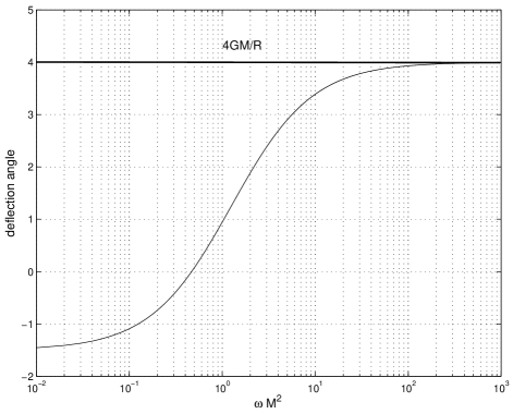
Figure 2: Deflection angle $\delta\varphi$ versus HL Gravity parameter $\omega M^{2}$ with $u_{0}=1$. The solid bold line denoted by $4GM/R$ is the usual Schwarzschild case [57].

V Constraints on Ho$\breve{r}$ava-Lifshitz Gravity from astronomical observations

In this section, we will use the observational data to confine the Ho$\breve{r}$ava-Lifshitz Gravity based on the deflection angle Eq.(34). It should be noticed that in order to analyse exactly the results Eq.(34), we move from the natural units used so far to the SI system by restoring $c$ and $G$ throughout the relevant formulas. In order to obtain experimental constraints from the light deflection result, the final light deflection angle $\delta\varphi$ should be expressed in terms of the deviation $\Delta_{LD}$ from the general relativity prediction $\delta\varphi_{GR}$ for the Sun.

$$\delta\varphi=\delta\varphi_{GR}(1+\Delta_{LD}),$$ (35)

where $\delta\varphi_{GR}=4GM/c^{2}R$. The best available constraints on $\delta\varphi_{GR}$ come from long-baseline radio interferometry which shows that $|\Delta_{LD}|\leq 0.0017$ by Robertson et al. Robertson and Lebach et al. Lebach . Submitting the deflection angles Eq.(34) into Eq.(35) and neglecting the higher-order terms, we can therefore infer an lower limit of Ho$\breve{r}$ava-Lifshitz gravity parameter

$$|\omega M^{2}|>8.27650\times 10^{-15},$$ (36)

for the solar system. However, it is important to bear in minds that the parameter $\omega$ characterizing the HL gravity metric (11) is not a naturally universal constant like $G$ or $c$, but it may in principle vary from one space to another. HL gravity as an alternative to 4D general relativity is therefore best constrained by the application of two or more tests to the same system.

With this in mind, according to the deviation $|\Delta_{LD}|\leq 0.17$ from the Jupiter measurement of light deflection by Treuhaft and Lowe Treuhaft , we can obtain

$$|\omega M^{2}|>8.27649\times 10^{-17}.$$ (37)

It has also been proposed by Gould Gould to measure the light deflection due to the Earth by using the Hipparcos satellite, with an estimated precision of $12\%$, which leads a sensitive values for the Earth system

$$|\omega M^{2}|>1.1725\times 10^{-16}.$$ (38)

VI comparison with others constrains from solar system and extrasolar planets

Here we compare our results with the constraints obtained by other researchers using solar system and exoplanetary data. The solar system tests include perihelion precessions Iorio1 ; Harko11 , radar echo delays and light bending Harko11 . The extrasolar planets have been recently used by Iorio and Ruggiero Iorio2 as well.

In the former classical solar system tests Harko11 , the constrains are obtained via the analysis of arbitrary spherically symmetric spacetimes Harko11 , which is different from the dynamic Lagrangian analysing in this paper. It should be noted that the parameters $\omega_{0}$ and $\psi_{0}$ used in Iorio1 ; Iorio2 ; Harko11 coincide with our $\omega M^{2}$. For the perihelion precession case, the circular orbit $u_{0}$ is determined by the nonlinear algebraic equation (51) in Ref. Harko11 which could bring us numerical solutions. So using the planet Mercury data, one can obtain the corresponding result $\omega M^{2}\sim 7\times 10^{-16}$ with the 43 arcsec per century of precession angle immediately, which is in the same order with our result of Hipparcos-Earth system, i.e. $1.2\times 10^{-16}$. For the radar echo delays case, the time interval between emission and return receiver is determined by the integration of lapse function,

$$\Delta t=\int_{-l_{1}}^{l_{2}}\bigg{\{}e^{\left[\lambda(\sqrt{y^{2}+R^{2}})-\nu(\sqrt{y^{2}+R^{2}})\right]/2}-1\bigg{\}}.$$ (39)

Though this general expression is simple, it is hard to solve and obtain a explicit form of time delays, except for the numerical solution, since there is a square root term in the KS lapse function. The numerical integration shows the result $\omega M^{2}\sim 4\times 10^{-15}$ which has an exact identical order of magnitude with our long-baseline radio interferometry result, i.e. $8.27650\times 10^{-15}$ under analytic analysis perspective. For the light deflection case, it is slightly emphasized that, in spite of considering light bending both in Ref.Harko11 and this paper, the based methods have nothing in common. Furthermore, the analysis of light bending based on the clear analytic expression of deflection angle (34) is grasped in this paper. Then, we have a look at the relating results in Ref. Harko11 . The photon’s motion equation satisfies the integral expression (55) of Ref. Harko11 . Hence, the deflection angle is $\Delta\phi=2|\phi(x_{0})-\phi(\infty)|-\pi$. Like the former radar echo delays case, since there are some square root terms, the numerical solution is obtained rather than analytic one. Submitting the classical observational value $\Delta\phi=1.7275$ arcsec, the result shows parameter $\omega_{0}=10^{-15}$, which is the same order as our results $\omega M^{2}\sim 8.3\times 10^{-15}$ based on the analytic perspective. Meanwhile, this results of the constraints on asymptotically flat IR modified Ho$\check{r}$ava gravity are compatible with the constraints in Jupiter and Earth systems. The corresponding compatibilities of parameter $\omega M^{2}$ are in the orders of $1\times 10^{-15}(\text{Harko\ and\ Kovacs})>8.27650\times 10^{-15}(\text{Solar\ \ system})>1.1725\times 10^{-16}(\text{Earth\ \ system})>8.27649\times 10^{-17}(\text{Jupiter\ \ system})$. Obviously, the constraints on Ho$\check{r}$ava gravity field parameter $\omega$ are more restrictive via the analytic method of this paper.

Then we consider the orbital motions tests Iorio1 ; Iorio2 in the following words. It should be noticed that in the approximation of weak field and slow motion, orbital motion mainly refers to the secular precession of the longitude for the pericenter test particle which has not perihelion at all. So orbital motion is different from that of the general relativistic Einstein’s pericentre precession. The constraints of orbital motion are divided into two parts, inside Iorio1 and outside Iorio2 our solar system. The secular precessions of the longitude of the pericentre $\varpi$ are calculated for a test particle by using the Gauss and Lagrange perturbative approaches. Then, based on the EPM2008 ephemerides constructed from a data set of 550000 observations ranging from 1913 to 2008 Pitjeva , they compared their results with the corrections $\Delta\dot{\varpi}$ to the standard Newtonian/ Einsteinian planetary perihelion precessions and found the lower bounds on KS solutions. For the case of solar system planets Iorio1 , inferior planets (Mercury, Venus, Earth, Mars) and outer planets (Jupiter, Saturn, Uranus, Neptune, Pluto), the lower limit of $\omega M^{2}$ is

$$|\psi_{0}|\geq\bigg{|}-\frac{3(GM)^{7/2}(4+e^{2})}{2\left[\Delta\dot{\varpi}\pm\delta(\Delta\dot{\varpi})\right]_{Max}c^{6}a^{9/2}(1-e^{2})^{3}}\bigg{|},$$ (40)

where $a$ is the semi-major axis and $e$ is the planet’s eccentricity. So the corresponding constraints on HL gravity ranging from $|\psi_{0}|\geq 10^{-12}$ to $|\psi_{0}|\geq 10^{-24}$ are shown in following tables Iorio1 . Interestingly, the larger value $8\times 10^{-12}$ in their work Iorio1 coming from Mercury is about 1000 times more than that of our result Eq.(36) coming from radio interferometry. For the same Earth, we also find that Iorio and Ruggiero’s result $6\times 10^{-14}$ is almost 513 times more than that of our result Eq.(38). In contrast, our result Eq.(37) is almost 30 times more than Iorio and Ruggiero’s result $3\times 10^{-18}$ for the same Jupiter plant.

Table 2: Lower bounds on $|\psi_{0}|$ of of the inner planets and outer planets in solar system Iorio1 .

inner	Mercury	Venus	Earth	Mars	—
planets	$8\times 10^{-12}$	$6\times 10^{-14}$	$6\times 10^{-14}$	$8\times 10^{-15}$	—
outer	Jupiter	Saturn	Uranus	Neptune	Pluto
planets	$3\times 10^{-18}$	$1\times 10^{-18}$	$2\times 10^{-22}$	$2\times 10^{-23}$	$8\times 10^{-24}$

Then we consider the other orbital motions type constraints coming from the extrasolar planets shown also by Iorio and Ruggiero Iorio2 . Like their early solar system work Iorio1 , the same standard Gauss perturbative approach was adopted. The correction to the Keplerian period is

$$P_{\omega_{0}}=\frac{4\pi(GM)^{5/2}(1+\frac{5}{4}e^{2})}{\omega_{0}c^{6}a^{3/2}(1-e^{2})^{5/2}},$$ (41)

where $\omega_{0}=\omega M^{2}=\psi_{0}$. By using the limit of $e\longrightarrow 0$, one can equates the centripetal acceleration to the Newton + KS gravitational acceleration for a circular orbit. The final expression of $\omega_{0}$ in HL gravity is

$$\omega_{0}=\frac{4\pi(GM)^{5/2}}{\Delta Pc^{6}d^{3/2}},$$ (42)

where $d$ represents the current fixed radius of the circular orbit and $\Delta P$ is the different value of correction orbital period to the third Kepler law. Comparing these with the phenomenologically determined orbital periods of the transiting extrasolar planet HD209458b “Osiris”, the result $\omega_{0}\geq 1.4\times 10^{-18}$ which is about one fiftieth of our minimum Jupiter planet value Eq.(37). Obviously, for the extrasolar planets give us a more rigorous constraints.

VII conclusion

In this paper, we have studied the constraints on HL gravity from light deflection astronomical observations including long-baseline radio interferometry Robertson ; Lebach , Jupiter measurement Treuhaft , Hipparcos satellite Gould . Here we summarize our findings.

We need briefly specify the parameters $\lambda$ and $\Lambda_{W}$ firstly. $\lambda$ is dimensionless coupling constant which controls the contribution of the extrinsic curvature trace. In this paper, we only consider the specific case of $\lambda=1$ which is corresponding to usual GR case at large distances. The parameter $\Lambda_{W}$ is the cosmological constant of HL gravity. For the various HL gravity models with Lifshitz points, $\Lambda_{W}$ has the different reduced values. For example, for $Z=1$ HL gravity in this paper, its value is $\Lambda_{W}=3\Lambda/2$ where $\Lambda$ is the cosmological constant of usual 4D GR. For $Z=4$ HL gravity, its values are $\Lambda_{W}=3\Lambda/2$ for (3 + 1) dimensions and $\Lambda_{W}=\Lambda$ for (4 + 1) dimensions CCai . Considering the asymptotically flat IR modified HL gravity, we adopt $\Lambda_{W}=0$ in this paper.

By using the conventional Lagrange approach for the calculus of variations, the the motion of photons is studied in the deformed HL gravity. The photons’ orbital equation (23) is coupled with the key HL Gravity parameter $\omega$ in the potential function $1/B^{2}(r)$. Hence, a scattering problem in a central force field occurs here. It is found that the photon collisional potential, which is larger for smaller $\omega$ is larger than in the usual GR case. Furthermore, for large values of $\omega$, the HL gravity reduces to the Schwarzschild case which is also justified by the Kehagias and Sfetsos’s Schwarzschild limit Kehagias .

All the classical tests in the solar system are in agreement with GR, especially those by long-baseline radio interferometry Robertson ; Lebach , Jupiter measurement Treuhaft , Hipparcos satellite Gould . So in this paper we use the Schwarzschild limit Kehagias and the difficult Eq.(25) is directly solved according to the linear superposition principle of ordinary differential equation. In the final result of Eq. (34), we find that the deflection angle value increases monotonically for large values of the HL gravity parameter $\omega M^{2}$ (or $\omega$). For a small magnitude of $\omega$ (about $10^{-17}\sim 10^{-15}$ here), the modification of HL gravity is dominated by the second term ($\sim 1/\omega$) according to Eq.(34). So the result of HL gravity is less than the usual GR value $4GM/R$. This relation of HL and GR is also clearly illustrated in FIG.2. The similar behavior will be found in the strong field gravitational lensing chensongbai1 ; Konoplya . Finally, the constraints on HL gravity from long-baseline radio interferometry Robertson ; Lebach , Jupiter measurement Treuhaft , Hipparcos satellite Gould are $|\omega M^{2}|>8.27650\times 10^{-15}$, $|\omega M^{2}|>8.27649\times 10^{-17}$ and $|\omega M^{2}|>1.1725\times 10^{-16}$ for Solar system, Jupiter system and Earth system, respectively.

For the comprehensive consideration of the constraints on asymptotically flat IR modified HL gravity, we also compare our results with others similar works including usual GR tests Harko11 , orbital motions inside Iorio1 and outsider Iorio2 solar system. Firstly, for the comparison with usual GR tests Harko11 , we find our constraint from Hipparcos-Earth system ($\sim 10^{-16}$) is concordant with the result of perihelion precession of Ref.Harko11 . Meanwhile, our constraint from long-baseline interferometry ($\sim 10^{-15}$) is in agreement with their result of radar echo delays case. However, for the same light deflection test, our results could give a more lower bound than their value ($\sim 10^{-15}$). Secondly, for the comparison with orbital motions inside solar system Iorio1 , we find that our result ($\sim 10^{-16}$) gives a lower bound, about two orders of magnitude, than that of their result ($\sim 10^{-14}$) for the same Earth system. However, our result ($\sim 10^{-15}$) gives a higher bound, about three orders of magnitude, than that of their result ($\sim 10^{-18}$) for the same Jupiter system. Thirdly, for the comparison with orbital motions outsider solar system Iorio2 , the lowest bound from our Jupiter case ($\sim 10^{-17}$) is higher one orders than that of HD209458b “Osiris” ($\sim 10^{-18}$). In general, according to the above situation, the HL gravity field parameter $\omega_{0}$ or $\psi_{0}$ should be in the range of $[10^{-12},10^{-24}]$. The constraint from solar system mainly concentrates in the range of $[10^{-17},10^{-15}]$, except for the orbital motions. On the contrary, the constraint from orbital motions distributes very separately, in which the largest bound ($\sim 10^{-12}$) and the lowest bound ($\sim 10^{-24}$) come from in Mercury system and Pluto system, respectively.

References

- (1) E. M. Lifshitz, On the Theory of Second-Order Phase Transitions I II, Zh. Eksp. Teor. Fiz 11 (1941)255 269.
- (2) P. Horava, Phys. Rev. D 79 (2009) 084008 (2009), [arXiv: 0901.3775].
- (3) P. Horava, Phys. Rev. Lett. 102 (2009) 161301, [arXiv: 0902.3657].
- (4) P. Horava, JHEP 0903 (2009) 020, [arXiv: 0812.4287].
- (5) T. P. Sotiriou, M. Visser and S. Weinfurtner, Phys. Rev. Lett. 102 (2009) 251601, [arXiv: 0904.4464].
- (6) M. Visser, Phys. Rev. D80 (2009) 025011, [arXiv: 0902.0590].
- (7) R. G. Cai, Y. Liu and Y. W. Sun, JHEP 0906 (2009) 010, [arXiv: 0904.4104].
- (8) B. Chen and Q. G. Huang, [arXiv: 0904.4565].
- (9) D. Orlando and S. Reffert, Class. Quant. Grav. 26 (2009) 155021, [arXiv: 0905.0301].
- (10) R. G. Cai, B. Hu and H. B. Zhang, Phys. Rev. D 80 (2009) 041501, [arXiv: 0905.0255].
- (11) T. Nishioka, [arXiv:0905.0473].
- (12) M. Li and Y. Pang, JHEP 08 (2009) 015, [arXiv: 0905.2751].
- (13) C. Charmousis, G. Niz, A. Padilla and P. M. Saffin, JHEP 0908 (2009) 070,[arXiv: 0905.2579].
- (14) T. P. Sotiriou, M. Visser and S. Weinfurtner, [arXiv: 0905.2798].
- (15) G. Calcagni, [arXiv: 0905.3740].
- (16) D. Blas, O. Pujolas and S. Sibiryakov, [arXiv: 0906.3046].
- (17) R. Iengo, J. G. Russo and M. Serone, [arXiv: 0906.3477].
- (18) C. Germani, A. Kehagias and K. Sfetsos, JHEP 09 (2009) 060, [arXiv: 0906.1201].
- (19) S. Mukohyama, JCAP 09 (2009) 005, [arXiv: 0906.5069].
- (20) C. Appignani, R. Casadio and S. Shankaranarayanan, [arXiv: 0907.3121].
- (21) J. Kluson, [arXiv: 0907.3566].
- (22) N. Afshordi, [arXiv: 0907.5201].
- (23) A. Kobakhidze, Phys. Rev. D 82 (2010) 064011, [arXiv: 0906.5401].
- (24) T. Takahashi, J. Soda, Phys. Rev. Lett. 102 (2009) 231301, [arXiv: 0904.0554].
- (25) E. Kiritsis and G. Kofinas, Nucl. Phys. B821 (2009) 467-480, [arXiv: 0904.1334].
- (26) S. Mukohyama, JCAP 0906, 001 (2009), [arXiv: 0904.2190].
- (27) R. Brandenberger, [arXiv: 0904.2835].
- (28) Y. S. Piao, [arXiv: 0904.4117].
- (29) S. Mukohyama, K. Nakayama, F. Takahashi and S. Yokoyama, [arXiv: 0905.0055].
- (30) S. Kalyana Rama, Phys. Rev. D79 (2009) 124031, [arXiv: 0905.0700].
- (31) B. Chen, S. Pi and J. Z. Tang, [arXiv: 0905.2300].
- (32) A. Wang and Y. Wu, JCAP 0907 (2009) 012, [arXiv: 0905.4117].
- (33) S. Nojiri and S. D. Odintsov, [arXiv: 0905.4213].
- (34) Y. F. Cai and E. N. Saridakis, [arXiv: 0906.1789].
- (35) A. Wang and R. Maartens, [arXiv: 0907.1748].
- (36) T. Kobayashi, Y. Urakawa and M. Yamaguchi, [arXiv: 0908.1005].
- (37) E. N. Saridakis, [arXiv: 0905.3532].
- (38) M. i. Park, [arXiv: 0906.4275].
- (39) S. Mukohyama, Phys. Rev. D 80 (2009) 064005, [arXiv: 0905.3563].
- (40) H. Nastase, [arXiv: 0904.3604].
- (41) R. G. Cai, L. M. Cao and N. Ohta, Phys. Rev. D 80 (2009) 024003, [arXiv: 0904.3670].
- (42) Y. S. Myung and Y. W. Kim, [arXiv: 0905.0179].
- (43) R. G. Cai, L. M. Cao and N. Ohta, Phys. Lett. B, 679 (2009) 504-509, [arXiv: 0905.0751].
- (44) R. B. Mann, JHEP 0906 (2009) 075, [arXiv: 0905.1136].
- (45) M. Botta-Cantcheff, N. Grandi and M. Sturla, [arXiv:0906.0582].
- (46) A. Castillo and A. Larranaga, [arXiv: 0906.4380].
- (47) J. J. Peng and S. Q. Wu, [arXiv: 0906.5121].
- (48) E. O. Colgain and H. Yavartanoo, JHEP 0908 (2009) 021, [arXiv: 0904.4357].
- (49) H. W. Lee, Y. W. Kim and Y. S. Myung, [arXiv: 0907.3568].
- (50) S. S. Kim, T. Kim and Y. Kim, [arXiv: 0907.3093].
- (51) M. i. Park, [arXiv: 0905.4480].
- (52) H. Lu, J. Mei and C. N. Pope, Phys. Rev. Lett. 103 (2009) 091301, [arXiv: 0904.1595].
- (53) A. Kehagias and K. Sfetsos, Phys. Lett. B 678 (2009) 123-126, [arXiv: 0905.0477].
- (54) G. Koutsoumbas, P. Pasipoularides, Phys. Rev. D 82, 044046 (2010), [arXiv:1006.3199].
- (55) G. Koutsoumbas, E. Papantonopoulos, P. Pasipoularides, M. Tsoukalas, Phys. Rev. D 81, 124014 (2010), [arXiv:1004.2289].
- (56) B. R. Majhi, Phys. Lett. B 686, 49 C54 (2010), [arXiv:0911.3239].
- (57) S. B. Chen and J. L. Jing, Phys. Rev. D 80 (2009) 024036, [arXiv: 0905.2055].
- (58) R. A. Konoplya, Phys. Lett. B 679 (2009) 499, [arXiv: 0905.1523].
- (59) S. B. Chen and J. L. Jing, [arXiv: 0905.1409].
- (60) J. H. Chen and Y. J. Wang, [arXiv: 0905.2786].
- (61) T. Harko, Z. Kovacs and F. S. N. Lobo, Phys. Rev. D 80 (2009) 044021, [arXiv: 0907.1449].
- (62) L. Iorio, M.L. Ruggiero, To appear in Int. J. Mod. Phys. A [arXiv:0909.2562].
- (63) L. Iorio, M.L. Ruggiero, [arXiv:0909.5355].
- (64) T. Harko, Z. Kovacs and F. S. N. Lobo, [arXiv:0908.2874].
- (65) D. Capasso and A.P. Polychronakos, JHEP 1002:068,2010, [arXiv:0909.5405].
- (66) S. K. Rama, Particle Motion with Horava-Lifshitz type Dispersion Relations, [arXiv:0910.0411].
- (67) A. E. Mosaffa, On Geodesic Motion in Horava-Lifshitz Gravity, [arXiv:1001.0490].
- (68) L. Sindoni, A note on particle kinematics in Horava-Lifshitz scenarios, [arXiv:0910.1329].
- (69) R. L. Arnowitt, S. Deser and C. W. Misner, [gr-qc/0405109].
- (70) Y. S. Myung, Phys. Lett. B 678 (2009) 127, [arXiv: 0905.0957].
- (71) R. M. Wald, General Relativity, the university of Chicago, Chicago. Sect. 6.3 (1984).
- (72) D.S. Robertson, W. E. Carter and W. H. Dillinger, Nature, 349 (1991) 768.
- (73) D. E. Lebach, B. E. Corey, I. I. Shapiro, M. I. Ratner, J. C. Webber, A. E. E. Rogers, J. L. Davis and T. A. Herring, Phys. Rev. Lett., 75 (1995) 1439.
- (74) R. N. Treuhaft and S. T. Lowe, AJ, 102 (1991) 1879.
- (75) A. Gould, ApJ, 414 (1993) L37.
- (76) E.V. Pitjeva, EPM ephemerides and relativity, in Relativity in Fundamental Astronomy: Dynamics, Reference Frames, and Data Analysis. Proceedings IAU Symposium No. 261, 2009 S.A. Klioner, P.K. Seidelman and M.H. Soffel, eds., pp. 170-178, 2010