Dynamical Casimir-Polder force on a partially dressed atom near a conducting wall

Abstract

We study the time evolution of the Casimir-Polder force acting on a neutral atom in front of a perfectly conducting plate, when the system starts its unitary evolution from a partially dressed state. We solve the Heisenberg equations for both atomic and field quantum operators, exploiting a series expansion with respect to the electric charge and an iterative technique. After discussing the behaviour of the time-dependent force on an initially partially-dressed atom, we analyze a possible experimental scheme to prepare the partially dressed state and the observability of this new dynamical effect.

I Introduction

According to quantum electrodynamics, the electric and magnetic fields show unavoidable fluctuations around their average values, even in the ground state of the field Milonni ; CPP95 . This feature gives rise to many physical phenomena such as the existence of a force between a couple of electrically neutral but polarizable objects. The existence of this kind of forces was first remarked by Casimir in 1948 for two parallel, neutral and perfectly conducting plates CasimirProcKonNederlAkadWet48 , and by Casimir and Polder for a neutral atom in front of a plate as well as between two neutral atoms CasimirPhysRev48 . The force between an atom and a surface, which is the main topic of this paper, has been measured with remarkable precision, notwithstanding the smallness of the force, using different techniques: deflection of atomic beams sent in proximity of surfaces SukenikPRL93 , reflection of cold atoms LandraginPRL96 ; ShimizuPRL01 ; DruzhininaPRL03 . More recently, Bose-Einstein condensates were exploited to obtain more precise measurements of the atom-surface force, using both reflection techniques PasquiniPRL04 ; PasquiniPRL06 and the observation of center-of-mass oscillations of the condensate AntezzaPRA04 ; HarberPRA05 ; AntezzaPRL06 ; ObrechtPRL07 .

The inclusion of dynamical (time-dependent) aspects in the system can considerably change the physical nature of the observed phenomena. When dealing with the dynamical Casimir-Polder effect, it is worthwhile distinguishing two different possible realizations of the dynamics. A first important situation to consider is the mechanical movement of the bodies of the system: in this case the emission of real photons can take place, having its dissipative counterpart in a friction force acting on the moving objects. This idea was first brought to attention in the pioneering works of Moore MooreJMathPhys76 and Fulling and Davies FullingProcRSocLondA76 , and then it paved the way to a remarkable amount of theoretical work (see DodonovArxiv and references therein). It does not yet exist any experimental observation of the emission of radiation by dynamical Casimir effect, due to the very low rate of photon emission, but a promising experiment is currently in progress in which the mechanical movement is replaced by the periodical modulation of the optical properties of one of the surfaces involved DodonovArxiv ; BraggioRevSciInstrum04 ; BraggioEurophysLett05 . On the other hand, the expression dynamical Casimir-Polder force is also used in the discussion of the time dependence of the force if the system undergoes a unitary evolution starting from a non-equilibrium quantum state PassantePhysLettA03 ; RizzutoPRA04 . For example, in PassantePhysLettA03 the authors studied the time evolution of the force between two neutral atoms starting from a partially dressed state of the system. Such a state is an intermediate configuration between the bare ground state of the system, which is given by the tensor product of the atomic ground state and the vacuum field state, and the physical, completely dressed, ground state of the composite system. Although the papers VasilePRA08 ; ShrestaPRA03 deal with the physical configuration we are interested in, that is a neutral atom in front of a conducting wall, the evolution is there studied starting from the bare ground state of the system, which is an idealized configuration hardly achievable in the laboratory.

In this paper we consider the evolution in time of the force between an atom and a perfectly conducting infinite plate starting from a partially dressed state, which is a much more realistic physical situation. To this aim, we are going to exploit, in analogy with VasilePRA08 , the method introduced by Power and Thirunamachandran PowerPRA83B for atoms in free space. It consists in solving the Heisenberg equations of the atomic and field operators in the Heisenberg picture by performing a series expansion with respect to the coupling constant (the electric charge) and then iteratively finding the solution (see PowerPRA83B or RizzutoPRA04 for more details). Then the time-dependent atom-wall Casimir-Polder energy is obtained for a specific model of a partially dressed atom, obtained by a rapid change of the atomic transition frequency due to an external action on the atom such as an external electric field PassantePhysLettA96 ; PassantePhysLettA03 . Finally, we discuss experimental realizability of the model considered and possibility of observing the dynamical effects predicted by our results.

This paper is organized as follows. In Section II we introduce the multipolar coupling scheme for a two-level atom interacting with the radiation field in the electric dipole approximation and in the presence of a conducting wall. Then we solve the Heisenberg equations for the photon creation and annihilation operators up to the first order in the electric charge, using an iterative technique, in order to obtain the Heisenberg operator giving the time-dependent atom-wall interaction energy. The solutions so obtained are valid for any initial state of the system. In Section III we discuss our choice of the initial state of the system, that is a partially dressed atomic state, and evaluate the time-dependent atom-wall interaction energy. Finally, in Sec. IV we discuss in more detail our physical model, its experimental realizability and the possible observation of the predicted dynamical Casimir-Polder interaction.

II The Hamiltonian model

We consider a two-level atom interacting with the electromagnetic radiation field in the presence of an infinite and perfectly conducting wall. We let the mirror coincide with the plane $z=0$ and we place the atom on its right side: the atomic position vector is thus $\mathbf{r}_{A}\equiv(0,0,d)$, with $d>0$. We work in the multipolar coupling scheme and within the electric dipole approximation (see e.g. PowerPhilTransRoySocA59 ; PowerPRA83A ). Thus the Hamiltonian describing our system reads

$$\begin{split}H&=H_{0}+H_{I}\\ H_{0}&=\hbar\omega_{0}S_{z}+\sum_{\mathbf{k}j}\hbar\omega_{\mathbf{k}}a^{{\dagger}}_{\mathbf{k}j}a_{\mathbf{k}j}\\ H_{I}&=-i\sqrt{\frac{2\pi\hbar c}{V}}\sum_{\mathbf{k}j}\sqrt{k}(\mbox{\boldmath$\mu$}\cdot\mathbf{f}_{\mathbf{k}j}(\mathbf{r}_{A}))\bigl{(}a_{\mathbf{k}j}-a^{{\dagger}}_{\mathbf{k}j}\bigr{)}\left(S_{+}+S_{-}\right).\end{split}$$ (1)

In this expression the radiation field is described by the set of bosonic annihilation and creation operators $a_{\mathbf{k}j}$ and $a^{{\dagger}}_{\mathbf{k}j}$, associated with a photon of frequency $\omega_{\mathbf{k}}=ck$, while the matrix element of the electric dipole moment operator $\mu$ and the pseudospin operators $S_{+}$, $S_{-}$ and $S_{z}$ are associated to the atom, which has a transition frequency $\omega_{0}$ CPP95 . Moreover $\mathbf{f}_{\mathbf{k}j}(\mathbf{r})$ are the field mode functions in the presence of the wall, that in Eq. (1) are evaluated at the atomic position $\mathbf{r_{A}}$. Their expressions can be obtained from the mode functions of a perfectly conducting cubical cavity of volume $V=L^{3}$ with walls ($-L/2<x,\;y<L/2$,  $0<z<L$) Milonni ; PowerPRA82

$$\begin{split}(\mathbf{f}_{\mathbf{k}j}(\mathbf{r}))_{x}&=\sqrt{8}(\hat{e}_{\mathbf{k}j})_{x}\cos\Bigl{[}k_{x}\Bigl{(}x+\frac{L}{2}\Bigr{)}\Bigr{]}\sin\Bigl{[}k_{y}\Bigl{(}y+\frac{L}{2}\Bigr{)}\Bigr{]}\sin\left(k_{z}z\right)\\ (\mathbf{f}_{\mathbf{k}j}(\mathbf{r}))_{y}&=\sqrt{8}(\hat{e}_{\mathbf{k}j})_{y}\sin\Bigl{[}k_{x}\Bigl{(}x+\frac{L}{2}\Bigr{)}\Bigr{]}\cos\Bigl{[}k_{y}\Bigl{(}y+\frac{L}{2}\Bigr{)}\Bigr{]}\sin\left(k_{z}z\right)\\ (\mathbf{f}_{\mathbf{k}j}(\mathbf{r}))_{z}&=\sqrt{8}(\hat{e}_{\mathbf{k}j})_{z}\sin\Bigl{[}k_{x}\Bigl{(}x+\frac{L}{2}\Bigr{)}\Bigr{]}\sin\Bigl{[}k_{y}\Bigl{(}y+\frac{L}{2}\Bigr{)}\Bigr{]}\cos\left(k_{z}z\right)\end{split}$$ (2)

where $k_{x}=l\pi/L$,  $k_{y}=m\pi/L$,  $k_{z}=n\pi/L$ ($l,m,n=0,1,2,\dots$) and $\hat{e}_{\mathbf{k}j}$ are polarization unit vectors. In order to switch from the cavity to the wall at $z=0$, at the end of the calculations one has to take the limit $L\rightarrow\infty$.

We are going to obtain all the information about the time evolution of the atom-wall force by solving the Heisenberg equations of all the atomic and field operators involved in our system. As anticipated before, since it is not possible to solve exactly these equations for our model, we shall use an iterative technique. As a starting point we write the operators as a power series in the coupling constant, that as an example for the annihilation operator takes the form

$$a_{\mathbf{k}j}(t)=a_{\mathbf{k}j}^{(0)}(t)+a_{\mathbf{k}j}^{(1)}(t)+a_{\mathbf{k}j}^{(2)}(t)+\dots$$ (3)

where the contribution $a_{\mathbf{k}j}^{(i)}(t)$ is proportional to the $i$-th power of the electric charge. For our purposes we need the expressions of both field and atomic operators up to the the first order only. The result is already reported in VasilePRA08 and it has the form

$$\begin{split}a_{\mathbf{k}j}^{(0)}(t)&=e^{-i\omega_{\mathbf{k}}t}a_{\mathbf{k}j}\qquad S_{\pm}^{(0)}(t)=e^{\pm i\omega_{0}t}S_{\pm}\\ a_{\mathbf{k}j}^{(1)}(t)&=e^{-i\omega_{\mathbf{k}}t}\sqrt{\frac{2\pi ck}{\hbar V}}\bigl{(}\mbox{\boldmath$\mu$}\cdot\mathbf{f}_{\mathbf{k}j}(\mathbf{r}_{A})\bigl{)}\bigl{[}S_{+}F(\omega_{\mathbf{k}}+\omega_{0},t)+S_{-}F(\omega_{\mathbf{k}}-\omega_{0},t)\bigl{]}\\ S^{(1)}_{\pm}(t)&=\mp 2S_{z}e^{\pm i\omega_{0}t}\sum_{\mathbf{k}j}\sqrt{\frac{2\pi ck}{\hbar V}}(\mbox{\boldmath$\mu$}\cdot\mathbf{f}_{\mathbf{k}j}(\mathbf{R}))\Bigl{(}a_{\mathbf{k}j}F^{*}(\omega_{\mathbf{k}}\pm\omega_{0},t)-a_{\mathbf{k}j}^{\dagger}F(\omega_{\mathbf{k}}\mp\omega_{0},t)\Bigr{)}.\\ \end{split}$$ (4)

where we have introduced the auxiliary function

$$F(\omega,t)=\int_{0}^{t}e^{i\omega t^{\prime}}dt^{\prime}=\frac{e^{i\omega t}-1}{i\omega}.$$ (5)

All operators appearing in the RHS of Eq. (4) without explicit time dependence are evaluated at $t=0$, and thus coincide with their counterpart in the Schrödinger picture. While the zeroth-order terms correspond to the absence of interaction and then to the free evolution given by $H_{0}$, the first-order terms couple the atomic and field operators. We wish to stress here the main advantage of solving the Heisenberg equations for the operators involved in the system: since in the Heisenberg picture only the operators evolve in time whilst the quantum state of the system remains constant, when calculating the time evolution of any average value the choice of the initial state can be performed just as a final step.

III Choice of the initial state and interaction energy

Our aim is to calculate the time-dependent atom-wall interaction energy, in particular for a partially dressed initial state. Using the same method as in VasilePRA08 , valid in a quasi-static approach at the second order, we shall calculate this quantity by taking half of the average value on the initial state of the interaction Hamiltonian $H_{I}^{(2)}(t)$ in the Heisenberg representation. Then we have

$$\Delta E^{(2)}(t)=\frac{1}{2}\displaystyle{\langle\psi(0)|}H^{(2)}_{I}(t)\displaystyle{|\psi(0)\rangle}$$ (6)

where $\displaystyle{|\psi(0)\rangle}$ is the initial state of the atom-field system. The explicit expression of $H_{I}(t)$ up to the second order is easily deduced from (1) and (4) (only atomic and field operators up to the first order are necessary), and it is given by

$$\begin{split}&H_{I}^{(2)}(t)=-\frac{2\pi ic}{V}\sum_{\mathbf{k}j}k\bigl{(}\mbox{\boldmath$\mu$}\cdot\mathbf{f}_{\mathbf{k}j}(\mathbf{r})\bigr{)}^{2}[S_{+}e^{i\omega_{0}t}+\text{h.c.}]\{S_{+}\\ &\,\times[e^{-i\omega_{\mathbf{k}}t}F(\omega_{0}+\omega_{\mathbf{k}},t)-e^{i\omega_{\mathbf{k}}t}F^{*}(\omega_{\mathbf{k}}-\omega_{0},t)]-\text{h.c.}\}\\ &\,+\frac{4\pi ic}{V}S_{z}\sum_{\mathbf{k}\mathbf{k^{\prime}}jj^{\prime}}\sqrt{kk^{\prime}}(\mbox{\boldmath$\mu$}\cdot\mathbf{f}_{\mathbf{k}j}(\mathbf{r}))(\mbox{\boldmath$\mu$}\cdot\mathbf{f}_{\mathbf{k^{\prime}}j^{\prime}}(\mathbf{r}))\\ &\,\times\{a_{\mathbf{k}^{\prime}j^{\prime}}[e^{i\omega_{0}t}F^{*}(\omega_{0}+\omega_{\mathbf{k^{\prime}}},t)-e^{-i\omega_{0}t}\\ &\,\times F^{*}(\omega_{\mathbf{k^{\prime}}}-\omega_{0},t)]+\text{h.c.}\}[a_{\mathbf{k}j}e^{-i\omega_{\mathbf{k}}t}-\text{h.c.}]\\ \end{split}$$ (7)

Now we must choose a specific initial quantum state to be used in (6). In VasilePRA08 the bare ground state was considered as initial state. This state is the eigenstate of $H_{0}$ having minimum energy: it accounts to a switching off of the interaction between atom and field and thus, although being a useful idealization, it is difficult to imagine an experimental scheme for generating such a state (but it can give important hints on the behaviour of more realistic systems). On the contrary, the completely dressed ground state of $H$ can be obtained by using stationary perturbation theory, and its expression up to the first order is given by

$$\begin{split}\displaystyle{|0_{d}\rangle}&=\displaystyle{|0\rangle}+\displaystyle{|1\rangle}\\ \displaystyle{|1\rangle}&=-i\sqrt{\frac{2\pi}{\hbar V}}\sum_{\mathbf{k}j}\frac{\sqrt{k}(\mbox{\boldmath$\mu$}\cdot\mathbf{f}_{\mathbf{k}j}(\mathbf{r}))}{k+k_{0}}\displaystyle{|1_{\mathbf{k}j},\uparrow\rangle}\end{split}$$ (8)

written as a sum of the bare ground state $\displaystyle{|0\rangle}$ and a sum of one-photon states gathered in $\displaystyle{|1\rangle}$. Up to the first order in the coupling constant, the state (8) does not undergo any time evolution. This expression clearly depends on the atomic transition frequency $ck_{0}$. This consideration is the basis of our proposal for the preparation of a partially-dressed state: we assume our atom initially to have a transition frequency $\omega_{0}^{\prime}$ and to be in its completely dressed ground state (given by (8) with $k_{0}^{\prime}$ in place of $k_{0}$), and then to produce at $t=0$ an abrupt change of its transition frequency from $\omega_{0}^{\prime}$ to a new frequency $\omega_{0}$. In the next Section we shall discuss in more detail how this rapid change of the atom’s transition frequency could be obtained. From the physical point of view, our hypothesis is that this change is so rapid that the quantum state immediately after $t=0$ remains the same as before. Thus this state will be taken as initial state of the unitary evolution for $t>0$, given by the Hamiltonian (1) with $\omega_{0}$ as the value of the atom’s transition frequency; this state is subjected to a time evolution because it is not an eigenstate of the new Hamiltonian at $t>0$, which is that for an atom with the new transition frequency $\omega_{0}$. A partially dressed state is so obtained PassantePhysLettA96 ; PassantePhysLettA03 .

We can now calculate three different average values of the interaction energy. The first is obtained starting from the completely dressed state of the system, given by (8): this state is a stationary state, and then we simply recover the well known result for the static atom-wall force. If, on the contrary, we consider the evolution from the bare ground state $\displaystyle{|0\!\downarrow\rangle}$, we indeed observe a time evolution of the atom-wall force, as obtained in VasilePRA08 . Finally, we can choose as initial state $\displaystyle{|\psi(0)\rangle}$ the dressed state (8) with a different transition frequency $\omega_{0}^{\prime}$, and also in this case a time evolution is expected. In all the three cases, the evolution is based on the Hamiltonian (1), according to which the atom has, for $t>0$, a transition frequency $\omega_{0}$ (while the transition frequency is $\omega_{0}^{\prime}$ for $t<0$) . The results obtained in all three different cases can be cast in the following compact form

$$\begin{split}\Delta E^{(2)}_{d}(d)&=\lim_{m\to 1}D_{m}\Bigl{[}\int_{0}^{+\infty}dx\frac{\sin(mx)}{x+x_{0}}\Bigr{]}\\ \Delta E^{(2)}_{b}(d,t)&=\lim_{m\to 1}D_{m}\Bigl{[}\int_{0}^{+\infty}dx\frac{\sin(mx)}{x+x_{0}}\Bigl{(}1-\cos[a(x+x_{0})]\Bigr{)}\Bigr{]}\\ \Delta E^{(2)}_{p}(d,t)&=\lim_{m\to 1}D_{m}\Bigl{[}\int_{0}^{+\infty}dx\frac{\sin(mx)}{x+x_{0}}\Bigl{(}1-\cos[a(x+x_{0})]\Bigr{)}+\int_{0}^{+\infty}\frac{\sin(mx)}{x+x^{\prime}_{0}}\cos[a(x+x_{0})]\Bigr{]}\\ \end{split}$$ (9)

where $a=ct/(2d)$, $x_{0}=2k_{0}d$, $x^{\prime}_{0}=2k^{\prime}_{0}d$, $x=2kd$ and $D_{m}$ is the differential operator

$$D_{m}=-\frac{\mu^{2}}{12\pi d^{3}}\Bigl{[}2-2\frac{\partial}{\partial m}+\frac{\partial^{2}}{\partial m^{2}}\Bigr{]}.$$ (10)

The three interaction energies $\Delta E^{(2)}_{d}(d)$, $\Delta E^{(2)}_{b}(d,t)$ and $\Delta E^{(2)}_{p}(d,t)$ in (9) are, respectively, for the fully dressed state, the bare state, and the partially dressed state cases. The second and third interaction energies reduce, as expected, to the first one for large values of $a$ (that is of $t$). Moreover, the third one coincides with the static expression for $k^{\prime}_{0}=k_{0}$, since in this case the initial state is the dressed ground state and then we do not expect any time evolution.

The integrals appearing in Eq. (9) can be calculated analytically and expressed in terms of the sine and cosine integral functions $\operatorname{Si}(x)$ and $\operatorname{Ci}(x)$ Abramowitz72 . The first and the third integrals yield respectively

$$\begin{split}&\int_{0}^{+\infty}dx\,\frac{\sin(mx)}{x+x_{0}}=\operatorname{Ci}(mx_{0})\sin(mx_{0})+\frac{1}{2}\cos(mx_{0})(\pi-2\operatorname{Si}(mx_{0}))\\ &\int_{0}^{+\infty}dx\,\frac{\sin(mx)}{x+x^{\prime}_{0}}\cos[a(x+x_{0})]=\frac{1}{4}\Bigl{[}-2\operatorname{Ci}[(a+m)x^{\prime}_{0}]\sin[a(x_{0}-x^{\prime}_{0})-mx^{\prime}_{0}]+2\operatorname{Ci}[l(a-m)x^{\prime}_{0}]\sin[a(x_{0}-x^{\prime}_{0})+mx^{\prime}_{0}]\\ &+\cos[a(x_{0}-x^{\prime}_{0})+mx^{\prime}_{0}](-l\pi+2\operatorname{Si}[(a-m)x^{\prime}_{0}])+\cos[a(x_{0}-x^{\prime}_{0})-mx^{\prime}_{0}](\pi-2\operatorname{Si}[(a+m)x^{\prime}_{0}])\Bigr{]}\end{split}$$ (11)

where $l=-1$ for $a<1$ $(t<2d/c)$ and $l=1$ for $a>1$ $(t>2d/c)$. The integral in the second line of Eq. (9) can be obtained by just taking $k_{0}^{\prime}=k_{0}$ in the second integral of Eq. (11). Applying the differential operator (10) and finally taking $m=1$, we get the analytic expression of the interaction energy, from which the atom-wall Casimir-Polder force can be obtained as the opposite of the derivative with respect to the distance $d$. These expressions are lengthy and not particularly enlightening from a physical point of view and thus will be not reported here explicitly.

One main point of this paper is the comparison between the time evolution of the force for the cases of an initial partially dressed state and an initial bare ground state, the latter already obtained in VasilePRA08 . In Figs. 1 and 2 we give the plots of the time evolution of the force for a bare ground state from VasilePRA08 (dashed blue lines) and for a partially dressed state as obtained from $\Delta E^{(2)}_{p}(d,t)$ in the third line of (9) (solid red lines). In both plots we take units such that $c=1$, and also $k_{0}=1$ and $k_{0}^{\prime}=2$; the atom is placed at a position such that $k_{0}d=10$. The difference between the values used for $k_{0}$ and $k_{0}^{\prime}$ is quite large, and it has be chosen in such a way just for the convenience of making more evident the qualitative different features obtained in the two cases considered. Fig. 1 refers to the region $a<1$, that is before a light signal leaving the atom at $t=0$ reaches to the wall and comes back, while Fig. 2 is for $a>1$. On the light cone instead ($a=1$) the force diverges: the physical meaning of this divergence, related to the well-known divergences of source fields and to the dipole approximation, has been already discussed in VasilePRA08 .

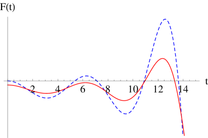
Figure 1: (color online). Time evolution of the atom-wall force for $t<2d$ ($c=1$). We have chosen $k_{0}=1$, $k^{\prime}_{0}=2$ and $d=10$, so that the back-reaction time is $t=20$. The red (solid) line corresponds to the case of an initial partially dressed state, while the blue (dashed) line is for the case of an initially bare ground state. Time is in units of $d/c$. The force is in arbitrary units.

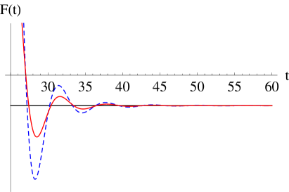
Figure 2: (color online). Time evolution of the atom-wall force for $t>2d$, with the same values and units of Fig. 1.

A first difference between the two cases (i.e. bare initial state and partially dressed initial state) is that the initial ($t=0$) value of the interaction energy for a partially dressed state is not zero. This happens because, when the system is in a partially dressed state at $t=0$, atom and field already see each other. It is interesting to analyze the time evolution towards the asymptotic regime (i.e. for $a>1$). We see, as expected, that the choice of a partially dressed initial state leads faster to the asymptotic value of the force, exhibiting nevertheless a similar oscillatory behavior around the asymptotic value. It is worth stressing that the asymptotic value of the force, when the atom becomes fully dressed, is the same in the two cases. This supports the hypothesis that in many aspects the dynamics towards the fully dressed state is indeed an irreversible process, with an equilibrium state independent from the initial state PassanteOC93 . The fact that different initial states, in general having different energies, lead for large times to the same atom-wall potential energy is not in contradiction with the energy-conserving unitary evolution of our system. The reason is that during the dynamical self-dressing of the atom, a spike of radiation propagates on the light cone from the atom and asymptotically in time it carries away part of the energy of the system to an infinite distance from the atom (see PassantePhysLettA03 ; CompagnoPRA88 for more detail). This energy is different for the cases considered (initially bare and partially dressed states), but it does not affect the large-time atom-wall interaction energy which is related to the field fluctuations at the atomic position; the latter at large times occurs to be the same in the cases considered.

An important point is that, similarly to what found in VasilePRA08 in the idealized case of an initial bare state, also in the more realistic case of an initial partially dressed atom, the force shows oscillations in time with negative (attractive) and positive (repulsive) values. This oscillation of the dynamical Casimir-Polder between an attractive and a repulsive character, in the case of the partially dressed atom can in principle be observed in the laboratory.

It is also significant to consider the evolution in time of the relative difference between the dynamical force we computed and its static value for $t\to+\infty$. We are thus going to consider the quantity

$$\frac{\Delta F(d,t)}{F(d)}=\frac{F_{p}(d,t)-F_{d}(d)}{F_{d}(d)}$$ (12)

with the same notations of Eq. (9). Fig. 3 represents a plot of $\Delta F(d,t)/F(d)$ with the same parameters as in Figs. 1 and 2.

Figure 3: Time evolution of the relative difference between the force for an initially partially dressed state and the stationary value for $t\to+\infty$. We have chosen $k_{0}=1$, $k^{\prime}_{0}=2$ and $d=10$ (and $c=1$). Time is in units of $d/c$.

As expected, this relative force difference oscillates in time and approaches zero for $t\to+\infty$. In the next Section we shall discuss the orders of magnitude of the physical parameters involved in the problem, as well as observability of this new effect, that is the time-dependent atom-wall Casimir-Polder force and its oscillatory behavior from an attractive to a repulsive character.

IV Discussion on the results

An essential point of our proposal outlined in the previous Section for generating an atomic partially dressed state is to produce an abrupt change of the atom’s transition frequency from $\omega_{0}^{\prime}$ to $\omega_{0}$. In the present Section we shall propose a possible method to realize this change and discuss the order of magnitude of the relevant parameters involved. A possible technique to produce a change of the atomic frequency is to place the atom at $t=0$ in a uniform electric field of amplitude $E_{0}$, as first suggested in PassantePhysLettA03 ; PassantePhysLettA96 . In this case, assuming that the old ($t<0$) free Hamiltonian of the system is

$$H^{\prime}_{0}=\hbar\omega_{0}^{\prime}S_{z}+\sum_{\mathbf{k}j}\hbar\omega_{\mathbf{k}}a^{{\dagger}}_{\mathbf{k}j}a_{\mathbf{k}j},$$ (13)

the new ($t>0$) Hamiltonian is

$$H_{0}=\hbar\omega_{0}S_{z}+\sum_{\mathbf{k}j}\hbar\omega_{\mathbf{k}}a^{{\dagger}}_{\mathbf{k}j}a_{\mathbf{k}j}$$ (14)

where the difference between the new and the old frequency is related to the amplitude $E_{0}$ of the electric field.

We now address the problem of the timescale of the switching on of the electric field, and in particular if it is compatible with our hypothesis that the quantum state of the system remains unchanged immediately after this process. A reliable estimate of a typical atomic evolution time is its inverse transition frequency $\tau=\omega_{0}^{-1}$. Thus our non-adiabatic hypothesis becomes reasonable if the time necessary to switch on the electric field is small compared to $\omega_{0}^{-1}$. Nevertheless, taking for example the case of an hydrogen atom in its ground state, we have $\tau=\omega_{0}^{-1}\simeq 10^{-15}\,$s which seems to be a quite short time to drive the electric field from zero to a value of $E_{0}$ sufficiently high to make appreciable our dynamical effects. This difficulty in the experimental realization of the model discussed in this paper, and the consequent observation of the dynamical Casimir-Polder force, could be overcome by considering a Rydberg atom, which can typically have a transition frequency of some GHz. In this case, switching on an electric field in times shorter than $\tau\sim 10^{-9}$ s should not be an impossible task (see Pelekanos95 ) and our assumptions should be valid. Our assumption of a stable atomic ground state should be also valid with a very good approximation in this case because Rydberg states can be long-lived atomic states. An alternative method to generate a partially dressed atomic state could be a rapid change of some other physical parameter of the atom significantly affecting its interaction with the radiation field, for example its refractive index. This could be obtained by an optical control such that obtained in Abdumalikov10 .

V Conclusions

We have considered the dynamical atom-wall Casimir-Polder force in a quasi-static approach for an initially partially dressed atom, and compared in detail the results obtained with the case of an initially bare state. A model for realizing the partially dressed atom, as well its limits, has been discussed. The time evolution of the atom-wall force has been calculated, and we have shown that it exhibits oscillations in time yielding to a oscillatory change of the Casimir-Polder force from an attractive to a repulsive character, and that asymptotically in time it settles to the value obtained in the stationary case. Possibility of experimental verification of our results has been also discussed.

- (1) P. W. Milonni, The Quantum Vacuum: An Introduction to Quantum Electrodynamics (Academic Press, San Diego, 1994)
- (2) G. Compagno, R. Passante, and F. Persico, Atom-Field Interactions and Dressed Atoms (Cambridge University Press, Cambridge, 1995)
- (3) H. B. G. Casimir, Proc. K. Ned. Akad. Wet. Ser. B 51, 793 (1948).
- (4) H. B. G. Casimir and D. Polder, Phys. Rev. 73, 360 (1948).
- (5) C. I. Sukenik, M. G. Boshier, D. Cho, V. Sandoghdar, and E. A. Hinds, Phys. Rev. Lett. 70, 560 (1993).
- (6) A. Landragin, J. Y. Courtois, G. Labeyrie, N. Vansteenkiste, C. I. Westbrook, and A. Aspect, Phys. Rev. Lett. 77, 1464 (1996).
- (7) F. Shimizu, Phys. Rev. Lett. 86, 987 (2001).
- (8) V. Druzhinina and M. DeKieviet, Phys. Rev. Lett. 91, 193202 (2003).
- (9) T. A. Pasquini, Y. Shin, C. Sanner, M. Saba, A. Schirotzek, D. E. Pritchard, and W. Ketterle, Phys. Rev. Lett. 93, 223201 (2004).
- (10) T. A. Pasquini, M. Saba, G. Jo, Y. Shin, W. Ketterle, D. E. Pritchard, T. A. Savas, and N. Mulders, Phys. Rev. Lett. 97, 093201 (2006).
- (11) M. Antezza, L. P. Pitaevskii, and S. Stringari, Phys. Rev. A 70, 053619 (2004).
- (12) D. M. Harber, J. M. Obrecht, J. M. McGuirk, and E. A. Cornell, Phys. Rev. A 72, 033610 (2005).
- (13) M. Antezza, L. P. Pitaevskii, S. Stringari, and V. B. Svetovoy, Phys. Rev. Lett. 97, 223203 (2006).
- (14) J. M. Obrecht, R. J. Wild, M. Antezza, L. P. Pitaevskii, S. Stringari, and E. A. Cornell, Phys. Rev. Lett. 98, 063201 (2007).
- (15) G. T. Moore, J. Math. Phys. 11, 2679 (1976).
- (16) S. A. Fulling and P. C. W. Davies, Proc. R. Soc. Lond. A 348, 393 (1976).
- (17) V. V. Dodonov, arXiv:1004.3301v1 (2010).
- (18) C. Braggio, G. Bressi, G. Carugno, A. Lombardi, A. Palmieri, and G. Ruoso, Rev. Sci. Instrum. 75, 4967 (2004).
- (19) C. Braggio, G. Bressi, G. Carugno, C. D. Noce, G. Galeazzi, A. Lombardi, A. Palmieri, G. Ruoso, and D. Zanello, Europhys. Lett. 70, 754 (2005).
- (20) R. Passante and F. Persico, Phys. Lett. A 312, 319 (2003).
- (21) L. Rizzuto, R. Passante, and F. Persico, Phys. Rev. A 70, 012107 (2004).
- (22) R. Vasile and R. Passante, Phys. Rev. A 78, 032108 (2008).
- (23) S. Shresta, B. L. Hu, and N. G. Phillips, Phys. Rev. A 68, 062101 (2003).
- (24) E. A. Power and T. Thirunamachandran, Phys. Rev. A 28, 2663 (1983).
- (25) R. Passante and N. Vinci, Phys. Lett. A 213, 119 (1996).
- (26) E. A. Power and S. Zineau, Phil. Trans. Roy. Soc. A 251, 427 (1959).
- (27) E. A. Power and T. Thirunamachandran, Phys. Rev. A 28, 2649 (1983).
- (28) E. A. Power and T. Thirunamachandran, Phys. Rev. A 25, 2473 (1982).
- (29) Handbook of Mathematical Functions, edited by M. Abramowitz and I. A. Stegun (Dover, New York, 1972).
- (30) R. Passante, T. Petrosky, I. Prigogine, Opt. Comm. 99, 55 (1993).
- (31) G. Compagno, R. Passante, F. Persico, Phys. Rev. A 38, 600 (1988).
- (32) N. T. Pelekanos, B. Deveaud, J. M. Gérard, H. Haas, U. Strauss, W. W. Rüle, J. Hebling, J. Kuhl, Optics Lett. 20, 2099 (1995).
- (33) A. A. Abdumalikov Jr., O. Astafiev, A. M. Zagoskin, Yu. A. Pashkin, Y. Nakamura, J. S. Tsai, Phys. Rev. Lett. 104, 193601 (2010).