Abstract

Dynamical systems that describe the escape from the basins of attraction of stable invariant sets are presented and analyzed. It is shown that the stable fixed points of such dynamical systems are the index-1 saddle points. Generalizations to high index saddle points are discussed. Both gradient and non-gradient systems are considered. Preliminary results on the nature of the dynamical behavior are presented.

1 The gentlest ascent dynamics

Given an energy function $V$ on $\mathbf{R}^{n}$, the simplest form of the steepest decent dynamics (SDD) associated with $V$ is

$$\dot{\mathbf{x}}=-\nabla V(\mathbf{x}).$$ (1)

It is easy to see that if $\mathbf{x}(\cdot)$ is a solution to (1), then $V(\mathbf{x}(t))$ is a decreasing function of $t$. Furthermore, the stable fixed points of the dynamics (1) are the local minima of $V$. Each local minimum has an associated basin of attraction which consists of all the initial conditions from which the dynamics described by (1) converges to that local minimum as time goes to infinity. For (1), these are simply the potential wells of $V$. The basins of attraction are separated by separatrices, on which the dynamics converges to saddle points.

We are interested in the opposite dynamics: The dynamics of escaping a basin of attraction. The most naive suggestion is to just reverse the sign in (1), the dynamics would then find the local maxima of $V$ instead. This is not what we are interested in. We are interested in the gentlest way in which the dynamics climb out of the basin of attraction. Intuitively, it is clear that what we need is a dynamics that converges to the index-1 saddle points of $V$. Such a problem is of general interest to the study of noise-induced transition between metastable states [3, 6] : Under the influence of small noise, with high probability, the escape pathway has to go through the neighborhood of a saddle point [5].

The following dynamics serves the purpose:

$$\dot{\mathbf{x}} =-\nabla V(\mathbf{x})+2\frac{(\nabla V,\mathbf{v})}{(\mathbf{v},\mathbf{v})}\mathbf{v},$$ (2a)

$$\dot{\mathbf{v}} =-\nabla^{2}V(\mathbf{x})\mathbf{v}+\frac{(\mathbf{v},\nabla^{2}V\mathbf{v})}{(\mathbf{v},\mathbf{v})}\mathbf{v}.$$ (2b)

We will show later that the stable fixed points of this dynamics are precisely the index-1 saddle points of $V$ and the unstable directions of $V$ at the saddle points. Intuitively the idea is quite simple: The second equation in (2) attempts to find the direction that corresponds to the smallest eigenvalue of $\nabla^{2}V$, and the last term in the first equation makes this direction an ascent direction.

This consideration is not limited to the so-called “gradient systems” such as (1). It can be extended to non-gradient systems. Consider the following dynamical system:

$$\dot{\mathbf{x}}=\mathbf{F}(\mathbf{x}).$$ (3)

We can also speak about the stable invariant sets of this system, and escaping basins of attraction of the stable invariant sets. In particular, we can also think about finding index-1 saddle points, though in this case, there is no guarantee that under the influence of small noise, escaping the basin of attraction has to proceed via saddle points[9].

For non-gradient systems, (2) has to be modified to

$$\dot{\mathbf{x}} =\mathbf{F}(\mathbf{x})-2\frac{(\mathbf{F}(\mathbf{x}),\mathbf{w})}{(\mathbf{w},\mathbf{v})}\mathbf{v},$$ (4a)

$$\dot{\mathbf{v}} =(\nabla\mathbf{F}(\mathbf{x}))\mathbf{v}-\alpha(\mathbf{v})\mathbf{v},$$ (4b)

$$\dot{\mathbf{w}} =(\nabla\mathbf{F}(\mathbf{x}))^{T}\mathbf{w}-\beta(\mathbf{v},\mathbf{w})\mathbf{w}.$$ (4c)

Here two directional vectors $\mathbf{v}$ and $\mathbf{w}$ are needed in order to follow both the right and left eigenvectors of the Jacobian. Given the matrix $\nabla\mathbf{F}(\mathbf{x})$, two scalar valued functions $\alpha$ and $\beta$ are defined by

$$\alpha(\mathbf{v}) =(\mathbf{v},(\nabla\mathbf{F}(\mathbf{x}))\mathbf{v}),$$ (5a)

$$\beta(\mathbf{v},\mathbf{w}) =2(\mathbf{w},(\nabla\mathbf{F}(\mathbf{x}))\mathbf{v})-\alpha(\mathbf{v}).$$ (5b)

We have taken and we will take the normalization such that $(\mathbf{v},\mathbf{v})=1$ and $(\mathbf{w},\mathbf{v})=1$. They are to keep the normalization such that $(\mathbf{v},\mathbf{v})=1$ and $(\mathbf{w},\mathbf{v})=1$. This normalization is preserved by the dynamics as long as it holds initially. Thus, the first equation in (4) actually is equivalent to $\dot{\mathbf{x}}=\mathbf{F}(\mathbf{x})-2{(\mathbf{F}(\mathbf{x}),\mathbf{w})}\mathbf{v}$. (Of course, one can enforce other types of normalization condition, such as the symmetric one: $(\mathbf{v},\mathbf{v})=(\mathbf{w},\mathbf{w})$ and $(\mathbf{w},\mathbf{v})=1$, and define new expressions of $\alpha$ and $\beta$ accordingly.) In the case of gradient flows, we can take $\mathbf{w}=\mathbf{v}$ and (4) reduces to (2).

Figure 1: Illustration of the gentlest ascent dynamics. $\mathbf{F}$ is the force of the original dynamics and $\tilde{\mathbf{F}}$ is the force of the gentlest ascent dynamics. $\mathbf{v}_{1}$ and $\mathbf{v}_{2}$ represent the unstable and stable right eigenvectors, respectively; $\mathbf{w}_{1}$ and $\mathbf{w}_{2}$ are the corresponding left eigenvectors. Note that $\mathbf{w}_{1}\perp\mathbf{v}_{2}$ and $\mathbf{w}_{2}\perp\mathbf{v}_{1}$. $\mathbf{F}$ has the decomposition $\mathbf{F}=\mathbf{F}_{1}+\mathbf{F}_{2}=c_{1}\mathbf{v}_{1}+c_{2}\mathbf{v}_{2}$ where the coefficient $c_{1}=(\mathbf{F},\mathbf{w}_{1})/(\mathbf{v}_{1},\mathbf{w}_{1})$. Thus, $\tilde{\mathbf{F}}:=-\mathbf{F}_{1}+\mathbf{F}_{2}=\mathbf{F}-2\mathbf{F}_{1}=\mathbf{F}-2c_{1}\mathbf{v}_{1}$.

We call this the gentlest ascent dynamics, abbreviated GAD. It has its origin in some of the numerical techniques proposed for finding saddle points. For example, there is indeed a numerical algorithm proposed by Crippen and Scheraga called the “gentlest ascent method” [2]. The main idea is similar to that of GAD, namely to find the right direction, the direction of the eigenvector corresponding to the smallest eigenvalue and making that an ascent direction. But the details of the gentlest ascent method seem to be quite a bit more complex. The “eigenvector following method” proposed in literature, for example, [1, 8], is based on a very similar idea. There at each step, one finds the eigenvectors of the Hessian matrix of the potential. Also closely related is the “dimer method” in which two states connected by a small line segment are evolved simultaneously in order to find the saddle point [7]. One advantage of the dimer method is that it avoids computing the Hessian of the potential. From the viewpoint of our GAD, the spirit of “dimer method” is equivalent to use central difference scheme to numerically calculate the matrix-vector multiplication in GAD (4) and (5) by writing $(\nabla\mathbf{F}(\mathbf{x}))\mathbf{b}=\frac{d}{d\varepsilon}\mathbf{F}(\mathbf{x}+\varepsilon\mathbf{b})|_{\varepsilon=0}\approx\frac{1}{2\varepsilon}(\mathbf{F}(\mathbf{x}+\varepsilon\mathbf{b})-\mathbf{F}(\mathbf{x}-\varepsilon\mathbf{b}))$ for any vector $\mathbf{b}$.

We believe that as a dynamical system, the continuous formulation embodied in (2) and (4) has its own interest. We will demonstrate some of these interesting aspects in this note.

Proposition. Assume that the vector field $\mathbf{F}$ is $C^{3}(\mathbf{R}^{n})$.

1. If $(\mathbf{x}_{*},\mathbf{v}_{*},\mathbf{w}_{*})$ is a fixed point of the gentlest ascent dynamics (4) and $\mathbf{v}_{*},\mathbf{w}_{*}$ are normalized such that $\mathbf{v}_{*}^{T}\mathbf{v}_{*}=\mathbf{v}_{*}^{T}\mathbf{w}_{*}=1$, then $\mathbf{v}_{*}$ and $\mathbf{w}_{*}$ are the right and left eigenvectors , respectively, of $\nabla\mathbf{F}(\mathbf{x}_{*})$ corresponding to one eigenvalue $\lambda_{*}$, i.e.,

   $$(\nabla\mathbf{F}(\mathbf{x}_{*}))\mathbf{v}_{*}=\lambda_{*}\mathbf{v}_{*},\quad(\nabla\mathbf{F}(\mathbf{x}_{*}))^{T}\mathbf{w}_{*}=\lambda_{*}\mathbf{w}_{*},$$

   and $\mathbf{x}_{*}$ is a fixed point of the original dynamics system, i.e., $\mathbf{F}(\mathbf{x}_{*})=\mathbf{0}$.

2. Let $\mathbf{x}_{s}$ be a fixed point of the original dynamical system $\dot{\mathbf{x}}=\mathbf{F}(\mathbf{x})$. If the Jacobian matrix $\mathbb{J}(\mathbf{x}_{s})=\nabla\mathbf{F}(\mathbf{x}_{s})$ has $n$ distinct real eigenvalues $\lambda_{1},\lambda_{2},\cdots,\lambda_{n}$ and $n$ linearly independent right and left eigenvectors, denoted by $\mathbf{v}_{i}$ and $\mathbf{w}_{i}$ correspondingly, i.e.,

   $$\mathbb{J}(\mathbf{x}_{s})\mathbf{v}_{i}=\lambda_{i}\mathbf{v}_{i},\qquad\mathbb{J}(\mathbf{x}_{s})^{T}\mathbf{w}_{i}=\lambda_{i}\mathbf{w}_{i},\quad i=1,\cdots,n$$

   and in addition, we impose the normalization condition $\mathbf{v}_{i}^{T}\mathbf{v}_{i}=\mathbf{w}_{i}^{T}\mathbf{v}_{i}=1,\ \forall i$ , then for all $i=1,\cdots,n$, $(\mathbf{x}_{s},\mathbf{v}_{i},\mathbf{w}_{i})$ is a fixed point of the gentlest ascent dynamics (4). Furthermore, among these $n$ fixed points, there exists one fixed point $(\mathbf{x}_{s},\mathbf{v}_{i^{\prime}},\mathbf{w}_{i^{\prime}})$ which is linearly stable if and only if $\mathbf{x}_{s}$ is an index-$1$ saddle point of the original dynamical system $\dot{\mathbf{x}}=\mathbf{F}(\mathbf{x})$ and the eigenvalue $\lambda_{i^{\prime}}$ corresponding to $\mathbf{v}_{i^{\prime}}$, $\mathbf{w}_{i^{\prime}}$ is the only positive eigenvalue of $\mathbb{J}(\mathbf{x}_{s})$.

Proof.

(a) Under the given condition, it is obvious that $(\nabla\mathbf{F}(\mathbf{x}_{*}))\mathbf{v}_{*}=\alpha(\mathbf{v}_{*})\mathbf{v}_{*}$ and $(\nabla\mathbf{F}(\mathbf{x}_{*}))^{T}\mathbf{w}_{*}=\beta(\mathbf{v}_{*},\mathbf{w}_{*})\mathbf{w}_{*}$. By definition and other conditions, $\beta(\mathbf{v}_{*},\mathbf{w}_{*})=2\mathbf{w}_{*}^{T}(\nabla\mathbf{F}(\mathbf{x}_{*}))\mathbf{v}_{*}-\alpha(\mathbf{v}_{*})=2\mathbf{w}_{*}^{T}(\alpha(\mathbf{x}_{*}))\mathbf{v}_{*}-\alpha(\mathbf{v}_{*})=\alpha(\mathbf{v}_{*})$. Therefore, $\mathbf{v}_{*}$ and $\mathbf{w}_{*}$ share the same eigenvalue $\lambda_{*}=\alpha(\mathbf{v}_{*})=\beta(\mathbf{v}_{*},\mathbf{w}_{*})$. From the fixed point condition $\mathbf{F}(\mathbf{x}_{*})-2(\mathbf{w}_{*}^{T}\mathbf{F}(\mathbf{x}_{*}))\mathbf{v}_{*}=\mathbf{0}$, we take the inner product of this equation with $\mathbf{w}_{*}$ to get $\mathbf{w}_{*}^{T}\mathbf{F}(\mathbf{x}_{*})=2\mathbf{w}_{*}^{T}\mathbf{F}(\mathbf{x}_{*})$. So $\mathbf{w}_{*}^{T}\mathbf{F}(\mathbf{x}_{*})=0$ and in consequence, the conclusion $\mathbf{F}(\mathbf{x}_{*})=\mathbf{0}$ holds from the fixed point condition $\mathbf{F}(\mathbf{x}_{*})-2(\mathbf{w}_{*}^{T}\mathbf{F}(\mathbf{x}_{*}))\mathbf{v}_{*}=\mathbf{0}$ again.

(b) It is obvious that for all $i$, $(\mathbf{x}_{s},\mathbf{v}_{i},\mathbf{w}_{i})$ is a fixed point of the gentlest ascent dynamics (4) by the definition of $\mathbf{v}_{i}$ and $\mathbf{w}_{i}$. It is going to be shown that we can explicitly write down the eigenvalues and eigenvectors of GAD at any fixed point $(\mathbf{x}_{s},\mathbf{v}_{i},\mathbf{w}_{i})$.

Let $\mathbb{J}(\mathbf{x})=\nabla\mathbf{F}(\mathbf{x})$. The Jacobian matrix of the gentlest ascent dynamics (4) has the following expression:  $\tilde{\mathbb{J}}(\mathbf{x},\mathbf{v},\mathbf{w})=$

$$\left(\begin{array}[]{ccc}(\mathbb{I}-2\mathbf{v}\mathbf{w}^{T})\mathbb{J}(\mathbf{x}),&-2(\mathbf{F}(\mathbf{x}),\mathbf{w})\mathbb{I},&-2\mathbf{v}\mathbf{F}(\mathbf{x})^{T}\\ \mathbb{L}_{1},&\mathbb{J}(\mathbf{x})-\alpha(\mathbf{v})\mathbb{I}-\mathbf{v}\mathbf{v}^{T}(\mathbb{J}(\mathbf{x})+\mathbb{J}(\mathbf{x})^{T}),&0\\ \mathbb{L}_{2},&-2\mathbf{w}\mathbf{w}^{T}\mathbb{J}(\mathbf{x})+\mathbf{w}\mathbf{v}^{T}(\mathbb{J}(\mathbf{x})+\mathbb{J}(\mathbf{x})^{T}),&\mathbb{J}(\mathbf{x})^{T}-\beta(\mathbf{v},\mathbf{w})\mathbb{I}-2\mathbf{w}\mathbf{v}^{T}\mathbb{J}(\mathbf{x})^{T}\\ \end{array}\right)$$ (6)

where $\mathbb{L}_{1}$, $\mathbb{L}_{2}$ are $n\times n$ matrices and $\mathbb{I}$ is the $n\times n$ identity matrix. To derive the above formula, we have used the results from (5) that $\nabla_{\mathbf{v}}(\alpha)=\mathbf{v}^{T}(\mathbb{J}^{T}+\mathbb{J})$, $\nabla_{\mathbf{v}}(\beta)=2\mathbf{w}^{T}\mathbb{J}-\mathbf{v}^{T}(\mathbb{J}^{T}+\mathbb{J})$ and $\nabla_{\mathbf{w}}(\beta)=2\mathbf{v}^{T}\mathbb{J}^{T}$ .

In the first $n$ rows of $\tilde{\mathbb{J}}$, there are two $n\times n$ blocks which contain the term $\mathbf{F}(\mathbf{x})$ and thus vanish at the fixed point $\mathbf{x}_{s}$. So the eigenvalues of $\tilde{\mathbb{J}}(\mathbf{x}_{s},\mathbf{v}_{i},\mathbf{w}_{i})$ can be obtained from the eigenvalues of its three $n\times n$ diagonal blocks: $\mathbb{N},\mathbb{M}$ and $\mathbb{K}$:

$$\begin{split}\mathbb{N}&=(\mathbb{I}-2\mathbf{v}_{i}\mathbf{w}_{i}^{T})\mathbb{J}(\mathbf{x}_{s}),\\ \mathbb{M}&=\mathbb{J}(\mathbf{x}_{s})-\lambda_{i}\mathbb{I}-\mathbf{v}_{i}\mathbf{v}_{i}^{T}(\mathbb{J}(\mathbf{x}_{s})+\lambda_{i}\mathbb{I}),\\ \mathbb{K}&=\mathbb{J}^{T}(\mathbf{x}_{s})-\lambda_{i}\mathbb{I}-2\mathbf{w}_{i}\mathbf{v}_{i}^{T}\mathbb{J}^{T}(\mathbf{x}_{s}).\end{split}$$

Here the obvious facts that $\alpha(\mathbf{v}_{i})=\beta(\mathbf{v}_{i},\mathbf{w}_{i})=\lambda_{i}$ and $\mathbf{v}_{i}^{T}\mathbb{J}^{T}=\lambda_{i}\mathbf{v}_{i}^{T}$ are applied.

Now we derive the eigenvalues of $\mathbb{N}$, $\mathbb{M}$ and $\mathbb{K}$ by constructing the corresponding eigenvectors. Note that $\mathbf{v}_{i}^{T}\mathbf{w}_{j}=\delta_{ij}$ holds under our assumption of the eigenvectors. One can verify that

$$\begin{split}\mathbb{N}\mathbf{v}_{i}&=(\mathbb{I}-2\mathbf{v}_{i}\mathbf{w}_{i}^{T})\lambda_{i}\mathbf{v}_{i}=-\lambda_{i}\mathbf{v}_{i},\\ \mathbb{M}\mathbf{v}_{i}&=-2\lambda_{i}\mathbf{v}_{i}\mathbf{v}_{i}^{T}\mathbf{v}_{i}=-2\lambda_{i}\mathbf{v}_{i},\\ \mathbb{K}\mathbf{w}_{i}&=-2\lambda_{i}\mathbf{w}_{i}\mathbf{v}_{i}^{T}\mathbf{w}_{i}=-2\lambda_{i}\mathbf{w}_{i},\\ \end{split}$$

and for all $j\neq i$,

$$\mathbb{N}\mathbf{v}_{j} = (\mathbb{I}-2\mathbf{v}_{i}\mathbf{w}_{i}^{T})\lambda_{j}\mathbf{v}_{j}=\lambda_{j}\mathbf{v}_{j},$$ (7)

$$\mathbb{K}\mathbf{w}_{j} = (\lambda_{j}-\lambda_{i})\mathbf{w}_{j}-2\lambda_{j}\mathbf{w}_{i}\mathbf{v}_{i}^{T}\mathbf{w}_{j}=(\lambda_{j}-\lambda_{i})\mathbf{w}_{j},$$ (8)

and with a bit more effort,

$$\begin{split}\mathbb{M}(\mathbf{v}_{j}-(\mathbf{v}_{i}^{T}\mathbf{v}_{j})\mathbf{v}_{i})&=\mathbb{M}\mathbf{v}_{j}-\mathbf{v}_{i}^{T}\mathbf{v}_{j}(\mathbb{M}\mathbf{v}_{i})=\mathbb{M}\mathbf{v}_{j}+2\lambda_{i}(\mathbf{v}_{i}^{T}\mathbf{v}_{j})\mathbf{v}_{i}\\ &=(\lambda_{j}-\lambda_{i})\mathbf{v}_{j}-(\lambda_{j}+\lambda_{i})\mathbf{v}_{i}(\mathbf{v}_{i}^{T}\mathbf{v}_{j})+2\lambda_{i}(\mathbf{v}_{i}^{T}\mathbf{v}_{j})\mathbf{v}_{i}\\ &=(\lambda_{j}-\lambda_{i})(\mathbf{v}_{j}-(\mathbf{v}_{i}^{T}\mathbf{v}_{j})\mathbf{v}_{i}).\end{split}$$ (9)

Hence the eigenvalues of the Jacobian $\tilde{\mathbb{J}}$ at any fixed point $(\mathbf{x}_{s},\mathbf{v}_{i},\mathbf{w}_{i})$ ($i=1,\cdots,n$) are

$$-2\lambda_{i},\ -\lambda_{i},\ \{\lambda_{j}:j\neq i\},\ \{\lambda_{j}-\lambda_{i}:j\neq i\}.$$ (10)

The first and last set of eigenvalues have multiplicity 2. The linear stability condition is that all numbers in (10) are negative. Thus one fixed point $(\mathbf{x}_{s},\mathbf{v}_{i^{\prime}},\mathbf{w}_{i^{\prime}})$ is linearly stable if and only if $\lambda_{i^{\prime}}>0$ and all other eigenvalues $\lambda_{j}<0$ for $j\neq i^{\prime}$, in which case the fixed point $\mathbf{x}_{s}$ is index-$1$ saddle.

Next, we discuss some examples of GAD.

Consider first the case of a gradient system with $V(\mathbf{x})=\mathbf{x}^{T}A\mathbf{x}/(\mathbf{x}^{T}\mathbf{x})$, where $A$ is a symmetric matrix. $V$ is nothing but the Rayleigh quotient. A simple computation shows that the GAD for this system is given by:

$$\left\{\begin{split}\dot{\mathbf{x}}=&-\frac{A\mathbf{x}}{\mathbf{x}^{T}\mathbf{x}}+\frac{\mathbf{x}^{T}A\mathbf{x}}{(\mathbf{x}^{T}\mathbf{x})^{2}}\mathbf{x}+2\left(\frac{\mathbf{v}^{T}A\mathbf{x}}{\mathbf{x}^{T}\mathbf{x}}-\frac{\mathbf{x}^{T}A\mathbf{x}}{(\mathbf{x}^{T}\mathbf{x})^{2}}(\mathbf{v}^{T}\mathbf{x})\right)\mathbf{v},\\ \dot{\mathbf{v}}=&-A\mathbf{v}+(\mathbf{v}^{T}A\mathbf{v})\mathbf{v}.\end{split}\right.$$ (11)

Next, we consider an infinite dimensional example. The potential energy functional is the Ginzburg-Landau energy for scalar fields: $I(u)=\int_{\Omega}\left(\frac{1}{2}|\nabla u|^{2}+\frac{1}{4}(u^{2}-1)^{2}\right)d\mathbf{x}$. The steepest decent dynamics in this case is described by the well-known Allen-Cahn equation:

$$\partial_{t}u=\Delta u-(u^{2}-1)u.$$ (12)

A direct calculation gives the GAD in this case:

$$\left\{\begin{split}\partial_{t}u&=\Delta u-(u^{2}-1)u-2(\Delta u-(u^{2}-1)u,v)v,\\ \partial_{t}v&=\Delta v-(3u^{2}-1)v-(\Delta v-(3u^{2}-1)v,v)v,\end{split}\right.$$ (13)

where the inner product is defined to be:

$$(u,v)=\int_{\Omega}u(\mathbf{x})v(\mathbf{x})d\mathbf{x}.$$

Clearly both the SDD and the GAD depend on the choice of the metric, the inner product. If we use instead the $H^{-1}$ metric, then the SDD becomes the Cahn-Hilliard equation and the GAD changes accordingly.

2 High index saddle points

GAD can also be extended to the case of finding high index saddle points. We will discuss how to generalize it to index-$2$ saddle points here. There are two possibilities: Either the Jacobian $\mathbb{J}$ at the saddle point has one pair of conjugate complex eigenvalues or it has two real eigenvalues at the saddle point. We discuss each separately.

Intuitively, the picture is as follows. We need to find the projection of the flow, $\mathbf{F}(\mathbf{x})$, on the tangent plane, say $P$, of the two dimensional unstable manifold of the saddle point, and change the direction of the flow on that tangent plane. For this purpose, we need to find the vectors $\mathbf{v}_{1}$ and $\mathbf{v}_{2}$ that span $P$. In the first case, we assume that the unstable eigenvalues at the saddle point are $\lambda_{1,2}=\lambda_{R}\pm i\lambda_{I}$. In this case there are no real eigenvectors corresponding to $\lambda_{1,2}$. However, for any vector $\mathbf{v}$ in $P$, $(\nabla\mathbf{F})\mathbf{v}$ simply rotates $\mathbf{v}$ inside $P$. Hence, $\mathbf{v}_{2}$ can be taken as $(\nabla\mathbf{F})\mathbf{v}_{1}$ if we have already found some $\mathbf{v}_{1}\in P$. The latter can be accomplished using the original dynamics in (4).

To see how one should modify the flow $\mathbf{F}$ on the tangent plane, we write

$$\mathbf{F}=c_{1}\mathbf{v}_{1}+c_{2}\mathbf{v}_{2}+\sum_{j>2}c_{j}\mathbf{v}_{j}.$$

Using the fact that the eigen-plane of $(\nabla\mathbf{F})^{T}$ corresponding to $\lambda_{R}\pm i\lambda_{I}$, which is spanned by $\mathbf{w}_{1}$ and $\mathbf{w}_{2}=(\nabla\mathbf{F})^{T}\mathbf{w}_{1}$, is orthogonal to $\mathbf{v}_{j}$ for all $j>2$, we can derive a linear system for $c_{1}$ and $c_{2}$ by taking the inner product of ${\mathbf{F}}$ and $\mathbf{w}_{1}$,$\mathbf{w}_{2}$. The solution of that linear system is given by:

$$c_{1}=\frac{a_{22}f_{1}-a_{12}f_{2}}{a_{11}a_{22}-a_{21}a_{21}},\ c_{2}=\frac{a_{11}f_{2}-a_{21}f_{1}}{a_{11}a_{22}-a_{21}a_{21}}$$ (14)

where $a_{ij}=(\mathbf{w}_{i},\mathbf{v}_{j})$ and $f_{j}=(\mathbf{F}(\mathbf{x}),\mathbf{w}_{j})$ for $i,j=1,2$. The gentlest ascent dynamics for the $\mathbf{x}$ component is

$$\tilde{\mathbf{F}}=\mathbf{F}-2c_{1}\mathbf{v}_{1}-2c_{2}\mathbf{v}_{2}.$$

To summarize, we obtain the following dynamical system:

$$\left\{\begin{split}\dot{\mathbf{x}}&=\mathbf{F}-2c_{1}\mathbf{v}_{1}-2c_{2}\mathbf{v}_{2},\\ \dot{\mathbf{v}}_{1}&=(\nabla\mathbf{F}(\mathbf{x}))\mathbf{v}_{1}-\alpha(\mathbf{v}_{1})\mathbf{v}_{1},\\ \dot{\mathbf{w}}_{1}&=(\nabla\mathbf{F}(\mathbf{x}))^{T}\mathbf{w}_{1}-\beta(\mathbf{v}_{1},\mathbf{w}_{1})\mathbf{w}_{1},\\ \mathbf{v}_{2}&=\nabla\mathbf{F}(\mathbf{x})\mathbf{v}_{1},\\ \mathbf{w}_{2}&=(\nabla\mathbf{F}(\mathbf{x}))^{T}\mathbf{w}_{1},\end{split}\right.$$ (15)

where $c_{1},c_{2}$ are given by (14) and $\alpha,\beta$ are defined by (5).

If the Jacobian has two positive real eigenvalues at the saddle point, say, $\lambda_{1}>\lambda_{2}>0\geq\lambda_{3}>\cdots$, let us define a new matrix by the method of deflation:

$$\mathbb{J}_{2}:=\nabla\mathbf{F}-\frac{(\mathbf{v}_{1},(\nabla\mathbf{F})\mathbf{v}_{1})}{(\mathbf{v}_{1},\mathbf{v}_{1})(\mathbf{w}_{1},\mathbf{v}_{1})}\mathbf{v}_{1}\mathbf{w}_{1}^{T}.$$ (16)

It is not difficult to see that if $\mathbf{v}_{1}$ is an eigenvector of $\nabla\mathbf{F}$ corresponding to $\lambda_{1}$, then ${\mathbb{J}}_{2}$ shares the same eigenvectors as $\mathbb{J}$, and the eigenvalues of $\mathbb{J}_{2}$ become $0,\lambda_{2},\lambda_{3},\cdots$. The largest eigenvalue of $\mathbb{J}_{2}$ at the index-$2$ saddle point becomes $\lambda_{2}$. One can then use the dynamics (4b) associated with the new matrix $\mathbb{J}_{2}$ to find $\mathbf{v}_{2}$. Therefore, we obtain the following index-$2$ GAD

$$\left\{\begin{split}\dot{\mathbf{x}}&=\mathbf{F}-2c_{1}\mathbf{v}_{1}-2c_{2}\mathbf{v}_{2},\\ \dot{\mathbf{v}}_{1}&=(\nabla\mathbf{F}(\mathbf{x}))\mathbf{v}_{1}-\alpha_{1}\mathbf{v}_{1},\\ \dot{\mathbf{w}}_{1}&=(\nabla\mathbf{F}(\mathbf{x}))^{T}\mathbf{w}_{1}-\beta_{1}\mathbf{w}_{1},\\ \dot{\mathbf{v}}_{2}&=\mathbb{J}_{2}\mathbf{v}_{2}-\alpha_{2}\mathbf{v}_{2},\\ \dot{\mathbf{w}}_{2}&=\mathbb{J}_{2}^{T}\mathbf{v}_{2}-\beta_{2}\mathbf{w}_{2},\end{split}\right.$$ (17)

with the initial normalization condition $(\mathbf{v}_{1},\mathbf{v}_{1})=(\mathbf{v}_{2},\mathbf{v}_{2})=(\mathbf{w}_{1},\mathbf{v}_{1})=(\mathbf{w}_{2},\mathbf{v}_{2})=1$. $c_{1}$ and $c_{2}$ are given in the same way as shown above (14) and $\alpha_{1,2},\beta_{1,2}$ are defined as follows to enforce that the normalization condition is preserved : $\alpha_{1}=(\mathbf{v}_{1},(\nabla\mathbf{F}(\mathbf{x}))\mathbf{v}_{1}),\beta_{1}=2(\mathbf{w}_{1},(\nabla\mathbf{F}(\mathbf{x}))\mathbf{v}_{1})-\alpha_{1}$ and $\alpha_{2}=(\mathbf{v}_{2},\mathbb{J}_{2}\mathbf{v}_{2}),\beta_{2}=2(\mathbf{w}_{2},\mathbb{J}_{2}\mathbf{v}_{2})-\alpha_{2}$.

The generalization to higher index saddle points with real eigenvalues is obvious.

3 Examples

3.1 Analysis of a gradient system

To better understand the dynamics of GAD, let us consider the case when a different relaxation parameter is used for the direction $\mathbf{v}$:

$$\left\{\begin{split}\dot{\mathbf{x}}&=-\nabla V(\mathbf{x})+2(\nabla V,\mathbf{v})\mathbf{v},\\ \tau\dot{\mathbf{v}}&=-\nabla^{2}V(\mathbf{x})\mathbf{v}+(\mathbf{v},\nabla^{2}V\mathbf{v})\mathbf{v}.\end{split}\right.$$

To simplify the discussions, we consider the limit as $\tau\to 0$. In this case, we obtain a closed system for $\mathbf{x}$:

$$\dot{\mathbf{x}}=-\nabla V(\mathbf{x})+2(\nabla V,\mathbf{v}(\mathbf{x}))\mathbf{v}(\mathbf{x}),$$ (18)

where $\mathbf{v}(\mathbf{x})$ is the eigenvector of $\nabla^{2}V(\mathbf{x})$ associated with the smallest eigenvalue. Now we consider the following two dimensional system:

$$V(x,y)=\frac{1}{4}(x^{2}-1)^{2}+\frac{1}{2}\mu y^{2}$$

where $\mu$ is a positive parameter. $\mathbf{x}_{\pm}=(\pm 1,0)$ are two stable fixed points and $(0,0)$ is the index-$1$ saddle point. The eigenvalues and eigenvectors of the Hessian at a point $\mathbf{x}=(x,y)$ are

$$\lambda_{1} =3x^{2}-1\text{ and }\mathbf{v}_{1}=(1,0),$$

$$\lambda_{2} =\mu\text{ and }\mathbf{v}_{2}=(0,1).$$

Therefore, the eigendirection picked by GAD is

$$\begin{cases}\mathbf{v}_{GAD}(\mathbf{x})=\mathbf{v}_{1},&\mbox{ if }|x|<\sqrt{\frac{1+\mu}{3}},\\ \mathbf{v}_{GAD}(\mathbf{x})=\mathbf{v}_{2},&\mbox{ if }|x|>\sqrt{\frac{1+\mu}{3}}.\end{cases}$$ (19)

Consequently, by defining

$$V_{1}(x,y)=-\frac{1}{4}(x^{2}-1)^{2}+\frac{1}{2}\mu y^{2},$$

and

$$V_{2}(x,y)=\frac{1}{4}(x^{2}-1)^{2}-\frac{1}{2}\mu y^{2},$$

we can write the gentlest ascent dynamics (18) in the form of a gradient system driven by the new potential:

$$V_{GAD}(\mathbf{x})=V_{1}(\mathbf{x})\cdot 1_{|x|<\sqrt{\frac{1+\mu}{3}}}(\mathbf{x})+V_{2}(\mathbf{x})\cdot 1_{|x|>\sqrt{\frac{1+\mu}{3}}}(\mathbf{x})$$ (20)

where $1_{\cdot}(\mathbf{x})$ is the indicator function. Note that $V_{GA{\color[rgb]{0,0,1}{D}}}$ is not continuous at the lines $x=\pm\sqrt{\frac{1+\mu}{3}}$. The point $(0,0)$ becomes the unique local minimum of $V_{1}$, with the basin of attraction $\{(x,y):-1<x<1\}$. Outside of this basin of attraction, the flow goes to $(x=\pm\infty,y=0)$ and the potential $V_{1}$ falls to $-\infty$ . For $V_{2}$, the point $(0,0)$ is the unique local maximum and all solutions go to $(x=\pm 1,y=\pm\infty)$.

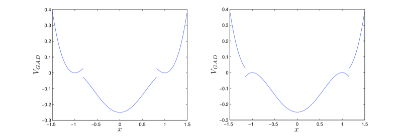
Figure 2: The discontinuity of $V_{GAD}(x,y=0)$ at the location $x=\pm\sqrt{\frac{1+\mu}{3}}$. Left: $\mu<2$; Right: $\mu>2$.

If we start the gentlest ascent dynamics with the initial value $\mathbf{x}_{\pm}=(\pm 1,0)$, then there are two different situations according to whether $\mu>2$ or $\mu<2$. Although $\mathbf{x}_{\pm}$ becomes a saddle point for any $\mu\neq 2$, the unstable direction for $\mu<2$ is $\pm\mathbf{v}_{2}$ while the unstable direction for $\mu>2$ is $\pm\mathbf{v}_{1}$, as illustrated in figure 3. Furthermore, from figure 3 and the above discussion, it is clear that the basin of attraction of the point $(0,0)$ associated with the potential $V_{GAD}$ is the region $-\sqrt{\frac{1+\mu}{3}}<x<\sqrt{\frac{1+\mu}{3}}$ for $\mu<2$ and $-1<x<1$ for $\mu>2$. (which is larger than the basin of attraction for the Newton-Raphson method, confirmed by numerical calculation.) Consequently, the GAD with an initial value $(x_{0},y_{0})$ near the local minimum $\mathbf{x}_{\pm}$ of $V$ converges to the point $(0,0)$ of our interest when $\mu>2$ and $|x_{0}|<1$.

This discuss suggests that GAD may not necessarily converge globally and instabilities can occur when GAD is used as a numerical algorithm. When instabilities do occur, one may simply reinitialize the initial position or the direction.

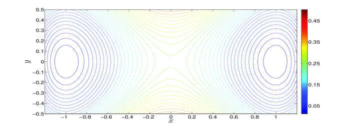
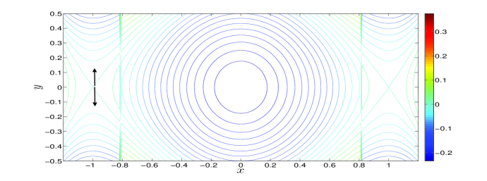
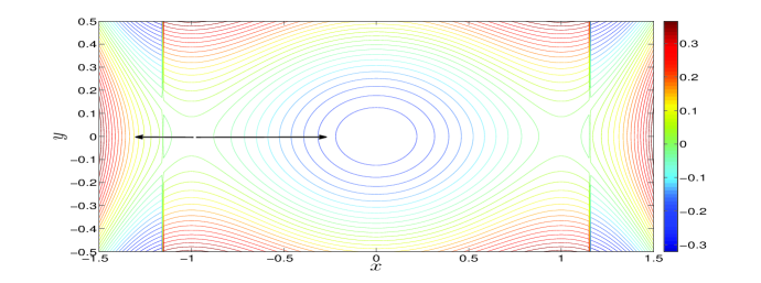
Figure 3: The contour plots of $V$, $V_{GAD}$ for $\mu=1$ and $V_{GAD}$ for $\mu=3$, from the top to the bottom, respectively. For the plot of $V_{GAD}$, $V_{1}$ lies in the middle region $-\sqrt{\frac{1+\mu}{3}}<x<\sqrt{\frac{1+\mu}{3}}$ and the $V_{2}$ lies at the two sides. The arrows show the flow directions of the gentlest ascent dynamics (18).

3.2 Lorenz system

Consider

$$\left\{\begin{array}[]{lcl}\dot{x}&=&\sigma(y-x),\\ \dot{y}&=&\rho x-y-xz,\\ \dot{z}&=&-\beta z+xy.\end{array}\right.$$ (21)

The parameters we use are $\sigma=10$, $\beta=\frac{8}{3}$ and $\beta=30$. There are three fixed points: the origin $O=(0,0,0)$ and two symmetric fixed points

$$Q_{\pm}=(\pm\sqrt{\beta(\rho-1)},\pm\sqrt{\beta(\rho-1)},\rho-1).$$

$O$ is an index-$1$ saddle point. The Jacobian at $Q_{\pm}$ has one pair of complex conjugate eigenvalues with positive real part. In our calculation, we prepare the initial directions $\mathbf{v}_{0}$ and $\mathbf{w}_{0}$ by running the GAD for long time starting from random initial conditions for $\mathbf{v}$ and $\mathbf{w}$ while keeping $\mathbf{x}$ fixed, although this is not entirely necessary. Figure  4 shows two solutions of GAD. For the index-$1$ saddle point $O$, figure 5 depicts how the trajectory of GAD converges to it. It can be seen that the component of the original force $\mathbf{F}$ along the unstable direction of $O$ is nearly projected out, thus the trajectory will not be affected by the unstable flow in that direction and avoids departing the saddle point. Therefore the trajectory tends to follow the stable manifold toward the saddle point when the trajectory is close enough to the saddle point. Similar behavior is seen for the case of searching the point $Q_{+}$ which has one pair of complex eigenvalues. The trajectory surrounding $Q_{+}$ in the figure 4 spirals to $Q_{+}$ and these spirals are closer and closer to the unstable manifold of $Q_{+}$ in the original Lorenz dynamics, which looks like a twisted disk. The convergence rate of the spiraling trajectories in GAD is very slow because the real part of the complex eigenvalues ($\lambda=0.1474\pm 10.5243\text{ i}$) in the original dynamics is rather small compared with its imaginary part.

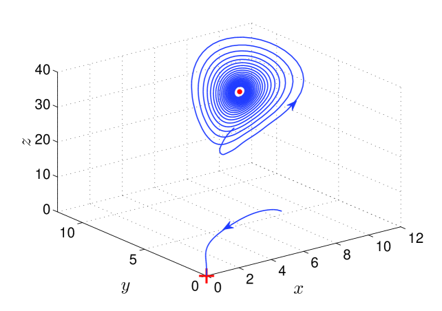
Figure 4: The trajectories of GAD for the Lorenz system starting from two initial points. They converge to the index-2 saddle point $Q_{+}$ (marked by the dot) and the index-1 saddle point $O$ (marked by “$+$”) respectively.

If we reverse time $t\to-t$, we have the time-reversed Lorenz system, in which the origin $O$ becomes an index-$2$ saddle point. We can apply the index-2 GAD algorithm (17) to search for this saddle point. The GAD trajectory in this case is also plotted in the figure 5. It is similar to the situation of GAD applied to the original Lorenz system in the sense that the GAD trajectory nearly follows the $z$ axis when approaching the limit point $O$. Indeed, as far as the $\mathbf{x}$-component is concerned, the linearized gentlest ascent dynamics for the original Lorenz system and the time-reversed one are the same. From the proof of the Proposition (particularly, note that the eigenvalues of $\mathbb{N}$ are $-\lambda_{i}$ and $\lambda_{j}$), it is not hard to see that the eigenvalues of the linearized gentlest ascent dynamics at the point $O$ are all negative and have the same absolute values as the eigenvalues of the original dynamics, and the two dynamics share the same eigenvectors (again, we mean the $\mathbf{x}$ component of the GAD). Thus, since the change $t\to-t$ does not change the absolute values of the eigenvalues of the original dynamics, the gentlest ascent dynamics for the original and time reversed Lorenz system have the same eigenvalues: $\lambda_{1}=-23.3955$, $\lambda_{2}=-2.6667$, $\lambda_{3}=-12.3955$. The two linearized GAD flows near the point $O$ are the same: $\mathbf{x}(t)=e^{-23.3955t}\mathbf{v}_{1}+e^{-2.6667t}\mathbf{v}_{2}+e^{-12.3995t}\mathbf{v}_{3}$, where $\mathbf{v}_{1,2,3}$ are the eigenvectors: $\mathbf{v}_{2}=(0,0,1)$, and $\mathbf{v}_{1}$, $\mathbf{v}_{3}$ are in the $z=0$ plane. As $t\to+\infty$, we then have $\mathbf{x}(t)\sim e^{-2.6667t}\mathbf{v}_{2}$. This explains why both trajectories in the figure 5 follow the $z$ axis when approaching the saddle point $O$.

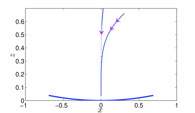
Figure 5: How the GAD trajectories approaches the saddle point $O$. The curve with two arrows is the trajectory of index-$1$ GAD for the Lorenz system; the curve with single arrow is the trajectory of index-$2$ GAD for the time reversed Lorenz system. The unstable manifold of $O$, which is tangent to the $z=0$ plane, is also shown.

3.3 A PDE example with nucleation

Let us consider the following reaction-diffusion system on the domain $x\in[0,1]$ with periodic boundary condition:

$$\left\{\begin{split}\frac{\partial u}{\partial t}&=\delta\Delta u+{\delta}^{-1}f(u,v),\\ \frac{\partial v}{\partial t}&=\delta\Delta v+{\delta}^{-1}g(u,v),\end{split}\right.$$ (22)

where

$$\begin{cases}f(u,v)&=(u-u^{3}+1.2)v+\frac{1}{2}\mu u,\\ g(u,v)&=\frac{1}{2}u^{2}-v.\end{cases}$$ (23)

The parameter $\delta$ is fixed at $0.01$ and we allow the parameter $\mu$ to vary. There are two stable (spatially homogeneous) solutions for certain range of $\mu$: $\mathbf{u}_{+}=(u_{+},v_{+})$ and $\mathbf{0}=(0,0)$. If one uses the square-pulse shape function as a initial guess in the Newton-Raphson method, no convergence can be achieved in most situations. We applied the index-$1$ GAD method to this example. The initial conditions for GAD are constructed by adding a small amount of perturbations around either stable solutions: $\mathbf{u}_{+}$ or $\mathbf{0}$. We observed that for a fixed value of $\mu$, the solutions of GAD constructed this way converge to the same saddle point. The different saddle points obtained from GAD at different values of $\mu$ are plotted in figure 6. It is also numerically confirmed that these saddle points indeed have index $1$ and the unstable manifold goes to $\mathbf{u}_{+}$ in one unstable direction and to $\mathbf{0}$ in the opposite unstable direction. It is interesting to observe the dependence of the saddle point on the parameter $\mu$ and that such a dependence is highly sensitive when $\mu$ is close to $-1.046\sim-1.045$. In fact, there exists a critical value $\mu^{*}$ in this narrow interval at which the spatially extended system (22) has a subcritical bifurcation, which does not appear in the corresponding ODE system without spatial dependence. We refer to [4] for further discussions about this point.

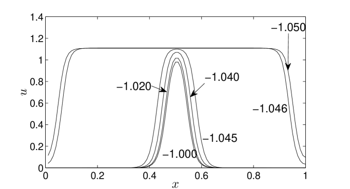
Figure 6: The profiles of saddle points of the example (23) ($\delta=0.01$). Only the component $u$ is shown since $v=\frac{1}{2}u^{2}$ at the saddle point. From inside to outside, the values of $\mu$ are $-1.000$, $-1.020$, $-1.040$, $-1.045$, $-1.046$, $-1.050$.

4 Concluding remarks

We expect that GAD is particularly useful for handling high dimensional system in the sense that it should have a larger basin of attraction for finding saddle points, than, for example, the Newton-Raphson method. There are many questions one can ask about GAD. One question is the convergence of GAD as time goes to infinity. Our preliminary result shows that GAD does not have to converge. For finite dimensional systems, there is always local convergence near the saddle point. The situation for infinite dimensional systems, i.e. PDEs, seems to be much more subtle. Another interesting point is whether one can accelerate GAD. For the problem of finding local minima, many numerical algorithms have been proposed and they promise to have much faster convergence than SDD. It is natural to ask whether analogous ideas can also be found for saddle points.

Acknowledgement: The work presented here was supported in part by AFOSR grant FA9550-08-1-0433. The authors are grateful to Weiguo Gao and Haijun Yu and the second referee for helpful discussions.

References

- [1] C. J. Cerjan and W. H. Miller, On finding transition states, J. Chem. Phys., 75 (1981), pp. 2800–2806.
- [2] G. M. Crippen and H. A. Scheraga, Minimization of polypeptide energy : Xi. the method of gentlest ascent, Arch. Biochem. Biophys., 144 (1971), pp. 462–466.
- [3] W. E, W. Ren, and E. Vanden-Eijnden, String method for the study of rare events, Phys. Rev. B, 66 (2002), p. 052301.
- [4] W. E and X. Zhou, Subcritical bifurcation in spatially extended systems, in preparation, (2011).
- [5] M. I. Freidlin and A. D. Wentzell, Random Perturbations of Dynamical Systems, Grundlehren der mathematischen Wissenschaften, Springer-Verlag, New York, 2 ed., 1998.
- [6] P. Hänggi, P. Talkner, and M. Borkovec, Reaction-rate theory: fifty years after Kramers, Rev. Mod. Phys., 62 (1990), pp. 251–341.
- [7] G. Henkelman and H. Jónsson, A dimer method for finding saddle points on high dimensional potential surfaces using only first derivatives, J. Chem. Phys., 111 (1999), pp. 7010–7022.
- [8] D. J. Wales, Energy Landscapes with Application to Clusters, Biomolecules and Glasses, Cambridge University Press, 2003.
- [9] X. Zhou, Noise-induce Transition Pathway in Non-gradient Systems, PhD thesis, Princeton University, 2009.