Origin of Molecular Outflow Determined from Thermal Dust Polarization

Abstract

The observational expectation of polarization measurements of thermal dust radiation is investigated to find information on molecular outflows based on magnetohydrodynamical (MHD) and radiation transfer simulations. There are two major proposed models for the driving of molecular outflows: (1) molecular gas is accelerated by a magnetic pressure gradient or magnetocentrifugal wind mechanism before the magnetic field and molecular gas are decoupled, (2) the linear momentum of a highly collimated jet is transferred to the ambient molecular gas. In order to distinguish between these two models, it is crucial to observe the configuration of the magnetic field. An observation of a toroidal magnetic field is strong evidence that the first of the models is appropriate. In this paper, we calculated the polarization distribution of thermal dust radiation due to the alignment of dust grains along the magnetic field using molecular outflow data calculated by two-dimensional axisymmetric MHD simulations. An asymmetric distribution around the $z$-axis is characteristic for magnetic fields composed of both poloidal and toroidal components. We determined that the outflow has a low polarization degree compared with the envelope and that the envelope and outflow have different polarization directions (B-vector), namely, the magnetic field within the envelope is parallel to the global magnetic field lines while the magnetic field of the outflow is perpendicular to it. Thus we have demonstrated that the point-symmetric (rather than axisymmetric) distributions of low polarization regions indicate that molecular outflows are likely to be magnetically driven. Observations of this polarization distribution with tools such as ALMA would confirm the origin of the molecular outflow.

1 Introduction

Magnetic fields play a crucial role in the star formation process. Magnetohydrodynamical (MHD) simulations have shown that molecular outflows and jets, which are ubiquitously observed in star forming regions, are launched by the magnetic Lorentz force (Tomisaka, 2002; Banerjee & Pudritz, 2006; Machida, Inutsuka & Matsumoto, 2007; Commerçon et al., 2010; Tomida et al., 2010). Furthermore, excess angular momentum of the molecular core of a star forming region is transferred by magnetic braking and the rotation rate is reduced to that observed for rotating stars (Tomisaka, 2000; Machida, Inutsuka & Matsumoto, 2007). However, the origin of molecular outflows has not yet been determined observationally. There are at least two major models for explaining molecular outflows. In the first model, the molecular outflow is accelerated by the magnetic Lorentz force, in the region in which the magnetic field and gas are well coupled (magnetically driven molecular outflow). This mechanism begins to work after the formation of the first core, which is the first hydrostatic object made of hydrogen molecules in the process of star formation (Larson, 1969), due to a combination of the magnetic field and rotational motion around the first core. Before the formation of the first core, or in the isothermal runaway collapse phase, no molecular outflow is launched. The second model is based on the idea that the jet is a primary object and its linear momentum is transferred to the ambient gas to form a bipolar molecular outflow (entrainment model). The well-collimated jet is thought to be magnetically accelerated (Shu et al., 1994; Kudoh, Matsumoto, & Shibata, 1998). In the entrainment model, the commonly observed wide opening angles in molecular outflows cannot be explained by the simple idea of momentum transfer (Stahler, 1993), since the jet is well collimated and its width is much smaller than that of the molecular outflow. A number of variations on the entrainment model have been proposed to address this problem, such as turbulent entrainment (Raga et al., 1993) and entrainment through a bow shock (Raga & Cabrit, 1993; Masson & Chernin, 1993). Comparisons are made between observed molecular outflows and models (Cabrit, Raga, & Gueth, 1997; Lee et al., 2000), which indicate that a part of the molecular outflows have observational signatures consistent with jet-driven origin. The magnetic drive model, however, can solve the angular momentum problem of newborn stars, as excess angular momentum, which must be greatly reduced to form stars, is removed to a distance by the magnetic torque and the molecular outflow (Tomisaka, 2000; Machida, Inutsuka & Matsumoto, 2007).

To explore the formation mechanism of molecular outflows, we need observational evidence to distinguish the above two models. The magnetically driven molecular outflow model predicts (1) rotation of the molecular outflow and (2) a toroidal magnetic field especially near the acceleration region. Although there are several observations of jet rotation (Chrysostomou et al., 2000; Davis et al., 2000; Bacciotti et al., 2002; Woitas et al., 2005; Coffey et al., 2007), only a few observations have been made on the rotation of molecular outflows. Launhardt et al. (2009) observed a molecular outflow around a T-Tauri star in a dark cloud named CB26 and found in an intensity-weighted velocity map of ${}^{12}{\rm CO}(J=2-1)$ that two lobes of the molecular outflow have systematic rotation with the same orientation as the high-density circumstellar disk rotation. This seems to indicate a twisted magnetic field due to the rotation of the high-density disk exerting a torque on the molecular material.

Further direct evidence of magnetic driven outflows is the existence of a strong toroidal magnetic field. The magnetic torque (or toroidal Lorentz force) arises from the combination of the poloidal current and poloidal magnetic field, and the poloidal current does not exist without a toroidal magnetic field. Thus, the magnetic acceleration region must be characterized by a toroidal magnetic field as well as a poloidal magnetic field. In the present paper, we demonstrate the characteristics of the configuration of a magnetic field driving the molecular outflow (i.e. a magnetic field consisting of both poloidal and toroidal components) in polarization observations of thermal dust emission.

If we compare these predictions with observations, we can distinguish which model is suitable for molecular outflows. This is done by post-processing the numerical results of an MHD simulation. We call this procedure “observational visualization,” which is a visualization process of the numerical results to explain the undergoing physics but also emphasizing the observational expectations from the simulation. In the observations of the magnetic field, we focus on the polarization of thermal dust radiation, which gives information about the configuration of the magnetic field. The strength of the magnetic field obtained from Zeeman splitting measurements will be presented in a future paper.

The plan of this paper is as follows: In section 2 we describe the molecular outflow model and summarize the results of MHD simulations. We also describe the numerical method for calculating the polarization of thermal dust radiation. In section 3, we present the results of the observation visualization. Section 4 is devoted to discussing the distribution of the polarization degree and the characteristic features of the magnetically driven molecular outflow.

2 Model and Method

We have presented calculations of the evolution of a rotating magnetized axisymmetric isothermal cloud in Tomisaka (2002), which is hereafter referred to as Paper I. In Paper I, we assumed a cloud in hydrostatic balance characterized by dimensionless parameters to specify the magnetic field strength, $\alpha=B_{z}^{2}/(4\pi\rho c_{s}^{2})$ ($B_{z}$, $\rho$, and $c_{s}$ are the magnetic flux density, gas density, and isothermal sound speed), and the rotation rate, $\Omega^{\prime}=\Omega_{0}\tau_{\rm ff}=\Omega_{0}/(4\pi G\rho_{s})^{1/2}$ ($\tau_{\rm ff}=1/[4\pi G\rho_{s}]^{1/2}$ represents the characteristic free-fall time-scale for the initial surface density of the cloud $\rho_{s}$, $\Omega_{0}$ represents the angular rotation speed at the center). Figure 1 illustrates the evolution of model AH1 from Paper I with $\alpha=1$ and $\Omega^{\prime}=5$. The parameters of this model correspond to a central density of $\rho_{c}=10^{4}{\rm H_{2}\,cm^{-3}}$, surface density of $\rho_{s}=10^{2}{\rm H_{2}\,cm^{-3}}$, magnetic field strength at the center of $B_{0}=13.3(\rho_{c}/10^{4}{\rm H_{2}\,cm^{-3}})^{1/2}\alpha^{1/2}{\rm\mu G}$, rotation rate at the center of $\Omega_{0}=2.78{\rm km\,s^{-1}\,pc^{-1}}(\Omega^{\prime}/5)$, and isothermal sound speed of $c_{s}=190{\rm m\,s^{-1}}$. The evolution is divided into two phases: before and after the first core formation. The figure shows the structure just before the first core formation (Fig. 1(a)) and when $\tau=3.94\times 10^{-3}\tau_{\rm ff}=7000{\rm yr}(\rho_{s}/100{\rm H_{2}cm^{-3}})^{-1/2}$ has passed after the first core formation (Fig. 1(b)). Before the first core forms, we observe a nested disk system composed of two disks, cocentered and bounded by different accretion shocks (the half thickness of the thinner disk is $z\simeq 0.01H\sim 700{\rm AU}(c_{s}/190{\rm m\,s^{-1}})(\rho_{s}/100{\rm H_{2}cm^{-3}})^{-1/2}$ and that of the thicker disk is $z\simeq 0.02H\sim 1400{\rm AU}(c_{s}/190{\rm m\,s^{-1}})(\rho_{s}/100{\rm H_{2}cm^{-3}})^{-1/2}$, where $H=7\times 10^{4}{\rm AU}(c_{s}/190{\rm m\,s^{-1}})(\rho_{s}/100{\rm H_{2}cm^{-3}})^{-1/2}$ represents the scale height of the initial cloud). This disk is actually a pseudodisk which continues to contract supersonically (Galli & Shu, 1993; Tomisaka, 1998). Just after the first core forms ($\tau\sim 1000{\rm yr}(\rho_{s}/100{\rm H_{2}cm^{-3}})^{-1/2}$), gas begins to be ejected around the core due to the centrifugal force driven by the extra angular momentum transferred by the magnetic tension force (magnetocentrifugal wind mechanism (Blandford & Payne, 1982)). At $\tau=7000{\rm yr}(\rho_{s}/100{\rm H_{2}cm^{-3}})^{-1/2}$, the outflow reaches $z\simeq 0.02H=1400{\rm AU}(c_{s}/190{\rm m\,s^{-1}})(\rho_{s}/100{\rm H_{2}\,cm^{-3}})^{-1/2}$ (Fig. 1(b)). For the kinetic temperature, we assume a barotropic gas: an isothermal envelope is assumed with $T_{K}=10\,\rm K$ for $\rho<\rho_{A}=10^{10}{\rm H_{2}cm^{-3}}$, although a hydrostatic core (the first core) with a small volume has a higher temperature as $T_{K}=10(\rho/\rho_{A})\,{\rm K}$ for $\rho>\rho_{A}=10^{10}{\rm H_{2}\,cm^{-3}}$.

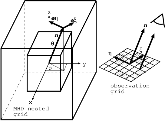
Figure 2: Relationship between the grid used in the MHD simulations (left: nested grid) and the observation grid (right). Observations were made by integrating along the normal vector $\boldsymbol{n}$. That is, the direction of the observation is specified by $\boldsymbol{n}$. The vertical and horizontal axes of the observation grid are chosen along the unit vectors $\boldsymbol{e}_{\eta}=\left[\boldsymbol{e}_{z}-(\boldsymbol{e}_{z}\cdot\boldsymbol{n})\boldsymbol{n}\right]/\left|\boldsymbol{e}_{z}-(\boldsymbol{e}_{z}\cdot\boldsymbol{n})\boldsymbol{n}\right|$ and $\boldsymbol{e}_{\xi}=\boldsymbol{e}_{\eta}\times\boldsymbol{n}$.

We then calculate the expected polarization distribution for thermal dust radiation observed from the direction $\boldsymbol{n}$. Figure 2 shows the relationship between the grid used in the MHD simulation (left) and the observation grid (right). The observation is made by integrating along the normal vector $\boldsymbol{n}$. The vertical and horizontal axes of the observation grid are chosen along the unit vectors

$$\boldsymbol{e}_{\eta} = \frac{\boldsymbol{e}_{z}-(\boldsymbol{e}_{z}\cdot\boldsymbol{n})\boldsymbol{n}}{\left|\boldsymbol{e}_{z}-(\boldsymbol{e}_{z}\cdot\boldsymbol{n})\boldsymbol{n}\right|},$$ (1)

$$\boldsymbol{e}_{\xi} = \boldsymbol{e}_{\eta}\times\boldsymbol{n}.$$ (2)

The vectors $\boldsymbol{n}$, $\boldsymbol{e}_{\xi}$, and $\boldsymbol{e}_{\eta}$ form a right-handed coordinate system and the direction of $\boldsymbol{e}_{\eta}$ is chosen to be toward the $z$-axis. The direction of $\boldsymbol{n}$ is specified by the angle $\theta$ from the $z$-axis of the simulation grid, along which the angular momentum and initial magnetic field are directed. Since the model is axisymmetric around the $z$-axis, the polarization is only dependent on the elevation angle $\theta$ and independent of the azimuth angle $\phi$. We will discuss the case without axisymmetry in a future study.

The polarization is calculated from the Stokes’ $Q$ and $U$ parameters. Assuming a constant emissivity per mass for dust, owing to the global isothermality in the molecular core and optically thin radiation, we substitute the relative Stokes’ parameters $q$ and $u$ for $Q$ and $U$ (Lee & Draine (1985); Fiege & Pudritz (2000); Matsumoto, Nakazato, & Tomisaka (2006)):

$$q = \int\rho\cos 2\psi\cos^{2}\gamma ds,$$ (3)

$$u = \int\rho\sin 2\psi\cos^{2}\gamma ds,$$ (4)

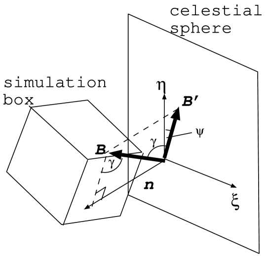
Figure 3: Relative Stokes’ parameter $q$ and $u$ calculated by integrating eqs (3) and (4) along $\boldsymbol{n}$. The angles used in eqs (3) and (4) are defined as follows: $\gamma$ and $\psi$ represent respectively the angle between the magnetic field and the plane of the sky and the angle between the projected magnetic field $\boldsymbol{B}^{\prime}$ and the $\eta$-axis.

where the integration is performed along the line-of-sight $\boldsymbol{n}$ and the two angles $\gamma$ and $\psi$ represent respectively that between the magnetic field and the plane of the sky and that between the projected magnetic field $\boldsymbol{B}^{\prime}$ and the $\eta$-axis (see Fig.3). From the relative Stokes’ parameters, we derive the polarization direction $\chi$ as

$$\cos 2\chi = \frac{q}{\left(q^{2}+u^{2}\right)^{1/2}},$$ (5)

$$\sin 2\chi = \frac{u}{\left(q^{2}+u^{2}\right)^{1/2}}.$$ (6)

Then, $\cos\chi$ and $\sin\chi$ are solved from equations (5) and (6) as

$$\cos\chi = \left(\frac{\cos 2\chi+1}{2}\right)^{1/2}$$ (7)

$$\sin\chi = \frac{\sin 2\chi}{2\cos\chi}\ \ \ ({\rm for}\ \cos\chi\neq 0),$$ (8)

where $\sin\chi=1$ (for $\cos\chi=0$) (see also Fiege & Pudritz (2000)). The polarization degree vector is calculated as

$$\boldsymbol{P}\equiv\left(\begin{array}[]{c}P_{\xi}\\ P_{\eta}\end{array}\right)=\left(\begin{array}[]{c}P\sin\chi\\ P\cos\chi\end{array}\right),$$ (9)

where $P$ represents the ratio of the polarized intensity to the total intensity and is given as

$$P=p_{0}\frac{\left(q^{2}+u^{2}\right)^{1/2}}{\Sigma-p_{0}\Sigma_{2}},$$ (10)

from the two integrated quantities

$$\Sigma \equiv \int\rho ds,$$ (11)

$$\Sigma_{2} \equiv \int\rho\left(\frac{\cos^{2}\gamma}{2}-\frac{1}{3}\right)ds.$$ (12)

The numerical factor $p_{0}$ is chosen to be $p_{0}=0.15$ to fit the maximum $P$ agreeing with the observations of typical dark clouds. The timescale of the alignment of the dust in the magnetized interstellar medium is not established, especially near the molecular core center where the gas is accelerated. Therefore, we assume the dust grains are aligned in a similar way to the dark cloud.

In conclusion, to calculate the polarization, we have to obtain four quantities ($u$, $q$, $\Sigma$, and $\Sigma_{2}$) integrating numerically along the line-of-sight (eqs.[3], [4], [11], and [12]). This is done on the nested grid hierarchy, in which $N$ levels of grid with different spatial resolutions are placed concentrically (see Paper I and Fig. 2). Figure 1 illustrates the $L=5$ level, which has $2^{5}=32$ times finer resolution than the $L=0$ level that covers the whole structure of the cloud. To make a polarization map with the same spatial resolution and the same spatial coverage as the $L=5$ grid, we integrate the above four equations (eqs.[4], [3], [11], and [12]) along the line-of-sight using all the data in grid levels $L=0,\ 1,\ \ldots,\ 5$. This is done by the following procedure with target=5:

    For L=0, target-1 do begin
      Integrate from outer to inner boundaries for grid level L
    End for
    Integrate for target grid level
    For L=target-1, 0, -1 do begin
      Integrate from inner to outer boundaries for grid level L
    End for

This procedure was tested by calculating the column density distribution obtained from a spherically symmetric density distribution $\rho(r)$, with the corresponding column density obtained by a numerical integration.

3 Result

3.1 Runaway Collapse Phase

In Figure 4, we plot the polarization at the final period of the isothermal runaway collapse phase just before the first core formation shown in Figure 1(a). The top row shows the distributions of the density and magnetic field seen in the nested grids for the $L=3$, $5$, $7$, and $9$ levels. These show that a pseudodisk in the form of a contracting disk forms in the direction perpendicular to the magnetic field in this phase. The other rows illustrate the polarization degree vectors, showing the directions of the B-vector and their polarization degree, as well as the column density (black contour lines) and polarization degree (false color and white contour lines). When a uniform magnetic field is deduced from the thermal dust emission, the radiation’s B-vector gives the direction of the magnetic field. The second to seventh rows represent the results for $\theta=0^{\circ}$ (along the $z$-axis or the pole-on view), $\theta=30^{\circ}$, $\theta=45^{\circ}$, $\theta=60^{\circ}$, $\theta=80^{\circ}$, and $\theta=90^{\circ}$ (the edge-on view), respectively.

Figure 4 shows that the polarization degree observed along the $z$-axis is much lower than that observed for $\theta\gtrsim 45^{\circ}$. The reason for this is clear: observing along the $z$-axis, the magnetic field runs perpendicular to the celestial plane, which greatly reduces $q$ and $u$ due to the fact that $\gamma\simeq 90^{\circ}$. In other words, dust grains do not align in a specific direction on the celestial plane.

In the range $30^{\circ}\leq\theta\leq 60^{\circ}$, a pseudodisk which is seen in the middle of the top panels is observed as an elliptical distribution of the column density (black contour lines), which is an effect of the projection. Although the polarization degree has its minimum near the major axis of the column density distribution, the minimum direction does not coincide with the major axis with a difference of $20^{\circ}-40^{\circ}$.

In Figure 4, models with $\theta\geq 80^{\circ}$ (near edge-on) exhibit an hour-glass shape, in which the magnetic field is squeezed near the mid-plane. However, it should be noted that the deviation from a straight magnetic field is small. The bottom panels show that the polarization degree varies depending on the heights from the mid-plane. Namely, a low polarization region extends over $500{\rm AU}\lesssim z\lesssim 1500{\rm AU}$ ($L=3$ and $5$). This corresponds to a post-shock region passing an accretion shock appearing at $z\sim 1500{\rm AU}$. In the pre-shock region $z\gtrsim 1500{\rm AU}$, the magnetic field line is essentially perpendicular to the pseudodisk, while in the post-shock region $B_{\phi}$ and $B_{r}$ are amplified due to compression. This configuration reduces the polarization degree in the post-shock region. Another accretion shock appears near $z\sim 10$–$20{\rm AU}$, of which the post-shock region corresponds to a low polarization degree around $|\eta|\sim 10$–$20{\rm AU}$ in the $L=9$ grid.

3.2 Accretion Phase

In Figure 5, we show the polarization obtained after the first core formation. As shown in the top row, the molecular outflow is ejected in this phase and the outflow reaches $z\simeq 2000{\rm AU}$ in $\tau\simeq 5000{\rm yr}(\rho_{s}/100{\rm H_{2}cm^{-3}})^{-1/2}$ after the core formation, which is seen in the $L=5$ grid. In the $L=7$ grid, gas moves outward in the region $200{\rm AU}\lesssim r\lesssim 400{\rm AU}$ at $z\sim 200{\rm AU}$, which is connected to a thick outflow lobe seen in the range $200{\rm AU}\lesssim r\lesssim 800{\rm AU}$ at the height $z\sim 1000{\rm AU}$.

Although the pole-on view ($\theta=0^{\circ}$) exhibits low polarization in Figure 4, the central part with radii $r\lesssim 500{\rm AU}$ has a larger polarization degree than the outer part, which is seen in the grids $L\geq 5$. This is due to the fact that the toroidal magnetic field is amplified by rotation of the disk at the mid-plane in contrast to the former runaway collapse phase.

The molecular outflow is clearly seen as a region with low polarization degree ($\lesssim 5\%$) extending vertically in the plots of $L=5$ for $\theta=60^{\circ}$–$90^{\circ}$ (compare the panels in the second column from the left). Outside the molecular outflow, the poloidal magnetic field is predominant, while inside the outflow the toroidal magnetic field is dominant. Since the poloidal magnetic field induces larger polarization than the toroidal one if we observe the outflow edge-on, the outflow is seen as a region with low polarization degree.

Although the disk is seen in a high polarization degree region in the edge-on view in the range $|\xi|\gtrsim 500~{}{\rm AU}$ ($L=3$ and $5$), the disk is composed of a region with low polarization degree looking further inside $|\xi|\lesssim 400~{}{\rm AU}$ ($L=7$). Disk rotation generates the toroidal magnetic field in this region, while outside $|\xi|\sim 500~{}{\rm AU}$ the poloidal magnetic field is dominant.

Between the pole-on and edge-on views ($30^{\circ}\leq\theta\leq 60^{\circ}$), a region with low polarization degree extends in the horizontal direction from the center, similar to the runaway collapse phase. The panels of $L=5$ for $30^{\circ}\leq\theta\leq 60^{\circ}$ contain a compact $\sim 200{\rm AU}$-scale region with high polarization degree. This is characteristic of the accretion phase, in contrast with the runaway collapse phase (Fig.4). This corresponds to the acceleration region where the toroidal magnetic field works to accelerate the gas. This region forms a spiral feature with a radius of $\sim 500$ AU, as seen for $L=7$.

3.3 Model with Weak Magnetic Field

In Figure 6, we plot the density and magnetic field lines in the accretion phase of a model with a weak magnetic field (model EH of Paper I; $\alpha=0.01$ and $\Omega^{\prime}=1$), which has a ten-times weaker magnetic field than the previous model. That is, the magnetic field strength at the center is equal to $B_{0}=1.33(\rho_{c}/10^{4}{\rm H_{2}\,cm^{-3}})^{1/2}(\alpha/0.01)^{1/2}{\rm\mu G}$ and the rotation rate at the center is equal to $\Omega_{0}=0.556{\rm km\,s^{-1}\,pc^{-1}}(\Omega^{\prime}/1)$, if the other parameters are taken to be the same. The rotation rate of this model is 1/5 that of the previous model. The outflow reaches $z\simeq 1200{\rm AU}$ in a time scale $\tau\sim 2\times 10^{4}\,{\rm yr}\,(\rho_{s}/100{\rm H_{2}\,cm^{-3}})^{-1/2}$. Owing to the weaker magnetic field (and relatively slow rotation), the density distribution looks nearly spherical (see the panel of $L=3$ in the top row). MHD simulations have already shown that the relatively weak magnetic field gives an outflow driven by the magnetic pressure gradient in the toroidal component and this outflow is well collimated. The strong magnetic field induces an outflow driven by the magnetocentrifugal wind, which has a wide opening angle (Kudoh, Matsumoto, & Shibata, 1998; Tomisaka, 2002). The model in this subsection corresponds to the model of outflows driven by the magnetic pressure gradient.

Similar to Figure 5, in Figure 6 the outflow is seen as a low-polarization region with $\sim 3\%$ ($L=5$ and $45^{\circ}\leq\theta\leq 90^{\circ}$). However, the outflow has an interior structure, which is also seen in the third column from the left, i.e., the $L=7$ grid. Near the rotation axis ($|\xi|\lesssim 200\,{\rm AU}$), a vertical structure with a relatively high polarization degree (10%) is seen. Since the polarization B-vector in this region is in the horizontal direction, it appears to arise from the toroidal magnetic field compressed near the $z$-axis. The toroidal field runs perpendicular to the celestial plane in the region $200~{}{\rm AU}\lesssim|\xi|\lesssim 600~{}{\rm AU}$, which reduces the polarization degree in this region.

In the edge-on view, a disk is traced as a region with high polarization $\sim 15\%$ ($\theta=90^{\circ}$ in the $L=3$ and $5$ levels). Similar to the previous model, a high polarization disk is truncated inside $|\xi|\lesssim 800{\rm AU}$. In this region, rotation and thus the toroidal magnetic field seem to predominate and reduce the polarization degree.

Between $\theta=30^{\circ}$ and $\theta=80^{\circ}$, a region with low polarization degree extends in the direction of the major axis of the column density distribution in the scale $L=3$ and $5$. Similar to the previous model, the direction of the low polarization degree and that of the major axis differ up to $\lesssim 30^{\circ}$.

4 Discussion

4.1 Origin of the Asymmetry

Although the distributions of both density and magnetic field are axisymmetric, the polarization distribution is not symmetric with respect to the $\eta$-axis. This seems strange at first glance. In this subsection, we consider this problem.

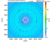
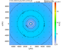
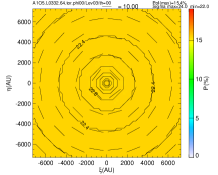
$\theta=45^{\circ}$                     

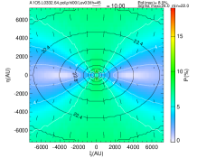
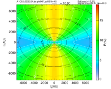
$\theta=90^{\circ}$                     

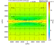
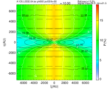
Figure 7: As for Fig. 4 (runaway collapse phase). However, the middle and right columns are results for artificial data consisting only of poloidal and toroidal magnetic fields, respectively. Level 3 of model AH1 with $\alpha=1$ and $\Omega^{\prime}=5$.

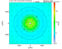
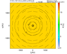
$\theta=45^{\circ}$                     

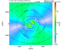
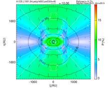
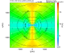
$\theta=90^{\circ}$                     

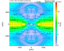
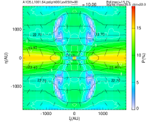
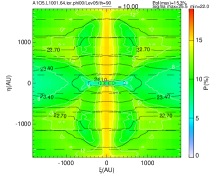
Figure 8: As for Fig. 5 (protostellar phases). However, the middle and right columns are results for artificial data consisting only of poloidal and toroidal magnetic fields, respectively. Level 5 of model AH1 with $\alpha=1$ and $\Omega^{\prime}=5$.

In Figures 7 and 8, we plot the expected polarization map for the model shown in Figures 4 and 5 (model AH1; $\alpha=1$ and $\Omega^{\prime}=5$). The left column is a plot of the results, while the middle and right columns are results obtained from artificial data consisting of the poloidal magnetic field without the toroidal field (middle: hereafter we call it a poloidal model) and from data consisting of the toroidal magnetic field without the poloidal field (right: hereafter we call it a toroidal model).

In the case of neither pole-on nor edge-on (i.e., $0^{\circ}<\theta<90^{\circ}$), the polarization degree distribution shown in the left column exhibits point symmetry rather than mirror symmetry. If we exclude the toroidal magnetic field (poloidal model) or exclude the poloidal magnetic field (toroidal model), we observe mirror symmetry with respect to the $\eta$-axis. Hence, only the true data, consisting of both the poloidal and toroidal magnetic fields, gives a polarization distribution without mirror symmetry. Namely, co-existing poloidal and toroidal magnetic fields induce this asymmetry.

The toroidal model (Figs. 7 and 8) exhibits a vertical bar structure with a strong polarization degree (the cases $\theta=45^{\circ}$ and $\theta=90^{\circ}$ of the toroidal model). Integrating the toroidal magnetic field, the polarization in the horizontal direction has a peak on the $\eta$-axis, since the magnetic field is parallel to the celestial plane and the column density has a maximum there. The distributions in the left and middle columns show some similarity, in contrast to the right column. For example, for $\theta=90^{\circ}$, a pseudodisk is observed with a similar structure, exhibiting a polarization degree decrease followed by an increase, rising from the mid-plane. This indicates that the magnetic field can be regarded essentially as being poloidal in this run-away collapse phase. Observing from $\theta=45^{\circ}$ in the direction of a major axis of the disk, the polarization degree is low.

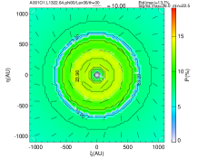
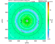
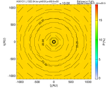
$\theta=45^{\circ}$                     

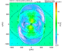
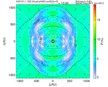
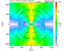
$\theta=90^{\circ}$                     

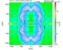
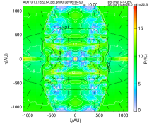
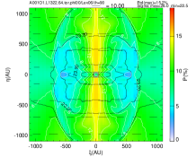
Figure 9: As for Fig. 6. However, the middle and right columns are results for artificial data consisting only of poloidal and toroidal magnetic fields, respectively. Level 6 of model EH with $\alpha=0.01$ and $\Omega^{\prime}=1$.

The polarization distributions in the accretion phase are shown in Figures 8 and 9, which correspond to models AH1 ($\alpha=1$ and $\Omega^{\prime}=5$) and EH ($\alpha=0.01$ and $\Omega^{\prime}=1$), respectively. In Figure 8, an outflow lobe is seen in the left column $\theta>0^{\circ}$ and also in the middle column as a low-polarization region. The fact that the lobe has a low polarization even in the poloidal model indicates that the low polarization is due to cancellation between the foreground and background. That is, the toroidal field component $B_{\phi}>0$ is mapped to a negative $B_{\xi}<0$ in the foreground but is mapped to a positive $B_{\xi}>0$ in the background.

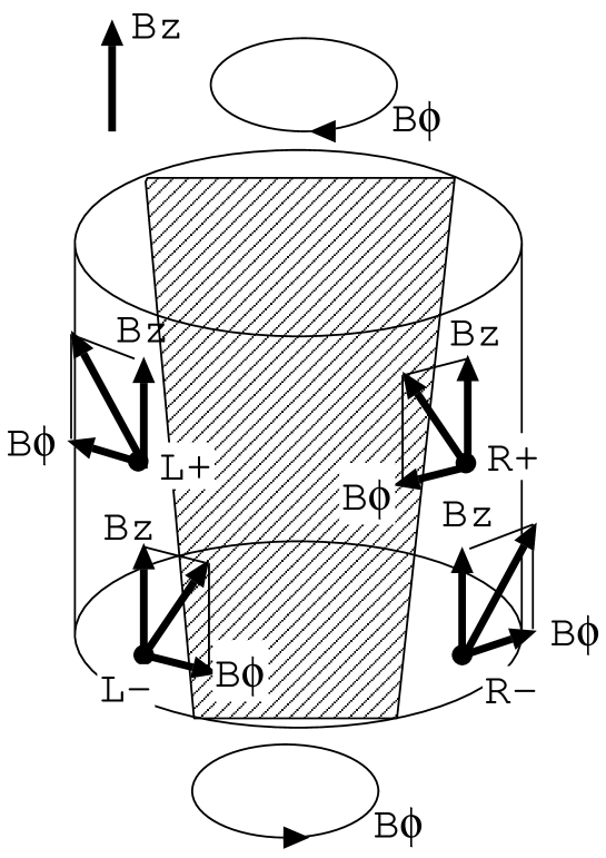
Figure 10: Illustration of the reason why mirror symmetry with respect to the $\eta$-axis is broken. For two points R$+$ and R$-$ at symmetric positions with respect to the midplane, if we assume that the magnetic field is composed of uniform $B_{z}$ and antisymmetric $B_{\phi}$ with respect to the midplane and the $\boldmath{B}$ vectors at R$+$ and R$-$ are projected on the celestial plane, the projected two vectors $\boldmath{B}^{\prime}$ have different amplitudes and are out of mirror symmetry. Considering the symmetric points with respect to the $\eta$-axis, L$+$ and L$-$, the projected $\boldmath{B}^{\prime}$ vectors at L$+$ and R$-$ are in point symmetry.

Figure 10 shows how the mirror symmetry breaks in a magnetic field consisting of poloidal and toroidal components. In this figure, we consider a magnetic field consisting of $B_{z}$ and $B_{\phi}$ and assume $B_{z}=$ const and $B_{\phi}$ changes its sign for $z>0$ and $z<0$, which is obtained when the outflow is ejected by the magnetic Lorentz force. Two points (R$+$ and R$-$) are taken at symmetric positions with respect to the mid-plane (and also L$+$ and L$-$). R and L are chosen to be symmetric with respect to the $\eta$-axis. Vectors of this magnetic field are projected onto a celestial plane for $\theta\simeq 45^{\circ}$. Looking from $0^{\circ}<\theta<90^{\circ}$, the projected vector $\boldsymbol{B}^{\prime}$ observed at R$+$ and R$-$ has different absolute values and points in different directions after the mirror reversal with respect to the $\xi$- or $\eta$-axes. The situation is the same for the vectors at L$+$ and L$-$. This explains how the mirror symmetry is broken.

4.2 Comparison with Observation

In the previous section we obtained the expected polarization map of thermal dust emission toward the prestellar core (Fig. 4, during the runaway collapse) and protostellar phase (Figs. 5 and 6). To distinguish the origin of the molecular outflow, it is essential to observe the toroidal magnetic field. The magnetically driven molecular outflow model induces a toroidal magnetic field with a strength at least comparable to the poloidal component, at that point and time where the molecular outflow is accelerated. This is obtained in a cloud core with a relatively strong magnetic field, $\alpha\sim 1$ shown in Figure 5. The magnetocentrifugal wind acceleration mechanism applies. In a molecular core with a weak magnetic field, $\alpha\ll 1$, the outflow is accelerated by the magnetic pressure gradient as shown in Figure 6. In this case, the strength of the toroidal component dominates the poloidal component in the molecular outflow. That is, the configuration of the magnetic field $|B_{\phi}|\gtrsim(B_{r}^{2}+B_{z}^{2})^{1/2}$ exhibits a characteristic signature of magnetically driven molecular outflow.

A toroidal dominant magnetic field gives a point-symmetric polarization distribution rather than a mirror-symmetric one. As we have found, a purely poloidal magnetic field recovers a mirror symmetry with respect to the $\eta-$axis. Thus, the predominance of a toroidal magnetic field is imprinted in the disk around the protostar. However, the direction of the major axis of the total intensity of the disk and the extension of the region with low polarization degree should first be compared. If the disk has a point symmetric polarization distribution rather than a mirror symmetric one, this indicates that a relatively strong toroidal magnetic field has been generated in the gaseous disk.

Another signature is a low polarization degree in the molecular outflow. If the coupling between dust and magnetic field is complete, this indicates a predominance of a toroidal magnetic field in the molecular outflow. Even if the dust alignment in the contracting envelope is the same as in the dark cloud, the alignment in the molecular outflow might be incomplete. Even in this case, the molecular outflow has to have a low polarization degree.

5 Summary

Based on two-dimensional axisymmetric MHD simulations, we calculated the polarization pattern expected in observations of thermal dust emission. We developed a procedure to calculate Stokes’ parameters on a nested grid hierarchy. The distribution of the polarization degree has an apparent signature indicating a toroidal component dominated magnetic field in the acceleration region of the molecular outflow. The outflow must have a lower polarization degree than the envelope. Another signature is imprinted on the disk whose rotation amplifies the toroidal magnetic field and thus accelerates the gas. A point-symmetric rather than a mirror-symmetric distribution of the low polarization degree region is another signature of a toroidal dominated magnetic field. If these characteristic features are observed, such a molecular outflow has toroidal-dominated magnetic field and is likely to be driven by the magnetic Lorentz force rather than the entrainment mechanism.

Figure Captions

(a)                                                            (b)

Figure 1: Structure of contracting magnetized rotating cloud in the prestellar (a) and poststellar (b) phases. This model corresponds to model AH1 of Paper I with $\alpha=1$ and $\Omega^{\prime}=5$. The solid lines illustrate the density contour and the dashed lines represent the magnetic field lines. The vectors show the velocity on the meridian plane.

($L=3$)                   ($L=5$)                   ($L=7$)                   ($L=9$)

$\theta=0^{\circ}$           

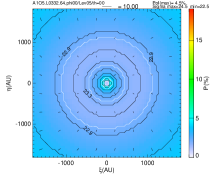
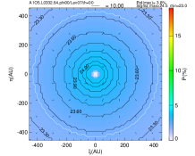
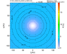
$\theta=30^{\circ}$         

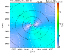
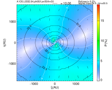
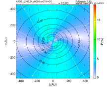
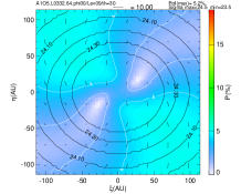
$\theta=45^{\circ}$         

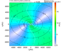
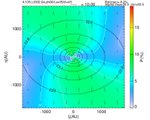
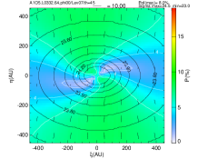
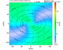
$\theta=60^{\circ}$         

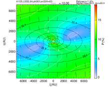
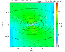
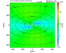
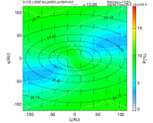
$\theta=80^{\circ}$         

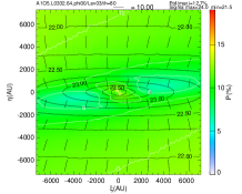
$\theta=90^{\circ}$         

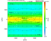
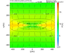
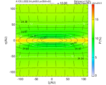
Figure 4: Expected polarization for the runaway collapse phase. Column density (black contour lines), polarization vector (bar), and polarization degree (false color and white contour lines) are shown for Levels 3, 5, 7, and 9 of model AH1 with $\alpha=1$ and $\Omega^{\prime}=5$. In the uppermost panels, density (solid line contours) and magnetic field lines (dashed line) are plotted.

($L=3$)                   ($L=5$)                   ($L=7$)                   ($L=9$)

$\theta=0^{\circ}$           

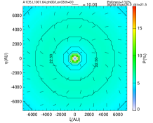
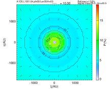
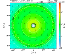
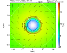
$\theta=30^{\circ}$         

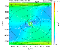
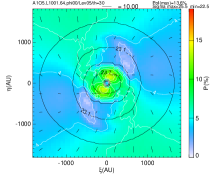
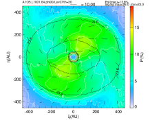
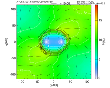
$\theta=45^{\circ}$         

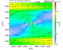
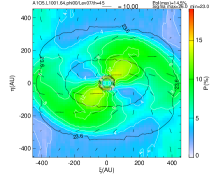
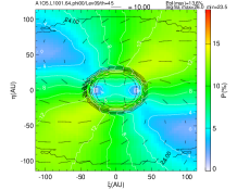
$\theta=60^{\circ}$         

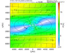
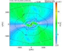
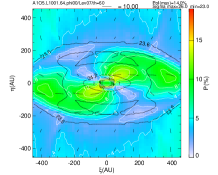
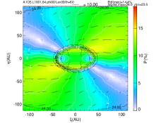
$\theta=80^{\circ}$         

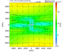
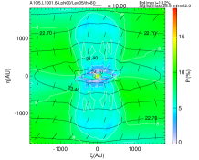
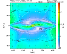
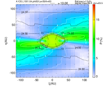
$\theta=90^{\circ}$         

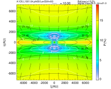
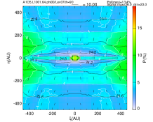
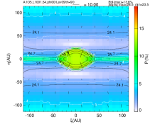
Figure 5: As for Fig.4 but for the accretion phase, in which the outflow is driven by the magnetic force.

($L=3$)                   ($L=5$)                   ($L=7$)                   ($L=9$)

$\theta=0^{\circ}$           

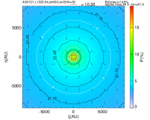
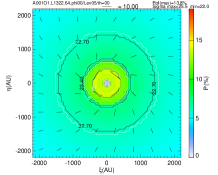
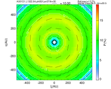
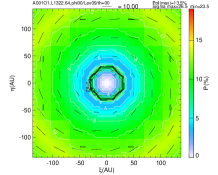
$\theta=30^{\circ}$         

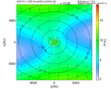
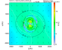
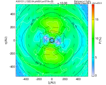
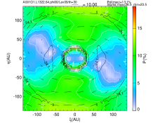
$\theta=45^{\circ}$         

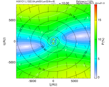
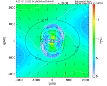
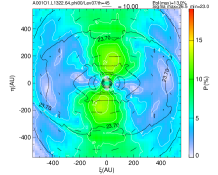
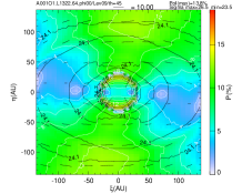
$\theta=60^{\circ}$         

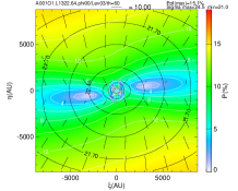
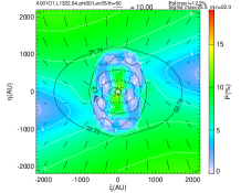
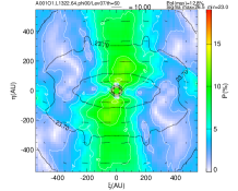
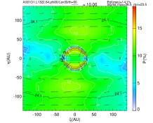
$\theta=80^{\circ}$         

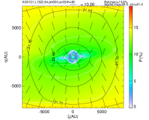
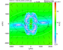
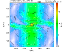
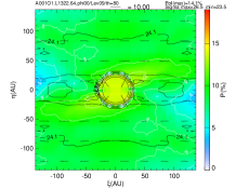
$\theta=90^{\circ}$         

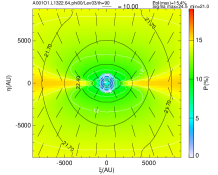
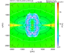
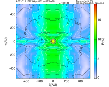
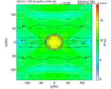
Figure 6: As for Fig.5 but for model EH with $\alpha=0.01$ and $\Omega^{\prime}=1$.

(poloidal)                          (toroidal)

$\theta=0^{\circ}$                       

(poloidal)                          (toroidal)

$\theta=0^{\circ}$                     

(poloidal)                          (toroidal)

$\theta=0^{\circ}$

References

- Bacciotti et al. (2002) Bacciotti, F., Ray, T. P., Mundt, R., Eislöffel, J., & Solf, J. 2002, ApJ, 576, 222
- Banerjee & Pudritz (2006) Banerjee, R., & Pudritz, R. E. 2006, ApJ, 641, 949
- Blandford & Payne (1982) Blandford, R. D., & Payne, D. G. 1982, MNRAS, 199, 883
- Cabrit, Raga, & Gueth (1997) Cabrit, S., Raga, A., & Gueth, F. 1997, in Herbig-Haro Flows and the Birth of Stars, ed. B. Reipurth, & C. Bertout (Kluwer Academic Publishers: Dordrecht) p.163.
- Coffey et al. (2007) Coffey, D., Bacciotti, F., Ray, T. P., Eislöffel, J., & Woitas, J. 2007, ApJ, 663, 350
- Chrysostomou et al. (2000) Chrysostomou, A., Hobson, J., Davis, C. J., Smith, M. D., & Berndsen, A. 2000, MNRAS, 314, 229
- Commerçon et al. (2010) Commerçon, B., Hennebelle, P., Audit, E., Chabrier, G., & Teyssier, R. 2010, A&A, 510, L3
- Davis et al. (2000) Davis, C. J., Berndsen, A., Smith, M. D., Chrysostomou, A., & Hobson, J. 2000, MNRAS, 314, 241
- Davis & Greenstein (1951) Davis, L., & Greenstein, J. L. 1951, ApJ, 114, 206
- Fiege & Pudritz (2000) Fiege, J. D., & Pudritz, R. E. 2000, ApJ, 544, 830
- Galli & Shu (1993) Galli, D., & Shu, F. H. 1993, ApJ, 417, 220
- Kudoh, Matsumoto, & Shibata (1998) Kudoh, T., Matsumoto, R., & Shibata, K. 1998, ApJ, 508, 186
- Larson (1969) Larson, R. B. 1969, MNRAS, 145, 271
- Launhardt et al. (2009) Launhardt, R., Pavlyuchenkov, Ya., Gueth, F., Chen, X., Dutrey, A., Guilloteau, S., Henning, Th., Piétu, V., Schreyer, K., & Semenov, D. 2009, A&A, 494, 147
- Lazarian (2007) Lazarian, A. 2007, J. Quant. Spec. Radiat. Transf., 106, 225
- Lazarian, & Draine (1999) Lazarian, A., & Draine, B. T. 1999, ApJ, 516, L37
- Lee & Draine (1985) Lee, H. M., & Draine, B. T. 1985, ApJ, 290, 211
- Lee et al. (2000) Lee, C.-F., Mundy, L. G., Reipurth, B., Ostriker, E. C., & Stone, J. M. 2000, ApJ, 542, 925 (erratum ApJ549, 1231)
- Machida, Inutsuka & Matsumoto (2007) Machida, M. N., Inutsuka, S.-I., & Matsumoto, T. 2007, ApJ, 670, 1198
- Masson & Chernin (1993) Masson, C. R., & Chernin, L. M. 1993, ApJ, 414, 230
- Matsumoto, Nakazato, & Tomisaka (2006) Matsumoto, T., Nakazato, T., & Tomisaka, K. 2006, ApJ, 637, L105
- Raga & Cabrit (1993) Raga, A., & Cabrit, S. 1993, A&A, 278, 267
- Raga et al. (1993) Raga, A. C., Canto, J., Calvet, N., Rodriguez, L. F., & Torrelles, J. M. 1993, A&A, 276, 539
- Shu et al. (1994) Shu, F., Najita, J., Ostriker, E., Wilkin, F., Ruden, S., & Lizano, S. 1994, ApJ, 429, 781
- Stahler (1993) Stahler, S. W., 1993 in Astrophysical Jets, ed. D. Burgarella, M. Livio, C. O’Dea (Cambbridge: Cambridge University Press)
- Tomida et al. (2010) Tomida, K., Tomisaka, K., Matsumoto, T., Ohsuga, K., Machida, M. N., & Saigo, K. 2010, ApJ,714, L58
- Tomisaka (1998) Tomisaka, K. 1998, ApJ, 502, L163
- Tomisaka (2000) Tomisaka, K. 2000, ApJ, 528, L41
- Tomisaka (2002) Tomisaka, K. 2002, ApJ, 575, 306
- Woitas et al. (2005) Woitas, J., Bacciotti, F., Ray, T. P., Marconi, A., Coffey, D., & Eislöffel, J. 2005, A&A, 432, 149