HETDEX pilot survey for emission-line galaxies - I. Survey design, performance, and catalog

Abstract

We present a catalog of emission-line galaxies selected solely by their emission-line fluxes using a wide-field integral field spectrograph. This work is partially motivated as a pilot survey for the upcoming Hobby-Eberly Telescope Dark Energy Experiment (HETDEX). We describe the observations, reductions, detections, redshift classifications, line fluxes, and counterpart information for 397 emission-line galaxies detected over 169 $\sq\arcmin$ with a 3500-5800Å bandpass under 5Å full-width-half-maximum (FWHM) spectral resolution. The survey’s best sensitivity for unresolved objects under photometric conditions is between $4-20\times 10^{-17}$ erg s^-1 cm^-2 depending on the wavelength, and Ly$\alpha$ luminosities between $3-6\times 10^{42}$ erg s^-1 are detectable. This survey method complements narrowband and color-selection techniques in the search for high redshift galaxies with its different selection properties and large volume probed. The four survey fields within the COSMOS, GOODS-N, MUNICS, and XMM-LSS areas are rich with existing, complementary data. We find 104 galaxies via their high redshift Ly$\alpha$ emission at $1.9<z<3.8$, and the majority of the remainder objects are low redshift [OII]3727 emitters at $z<0.56$. The classification between low and high redshift objects depends on rest frame equivalent width, as well as other indicators, where available. Based on matches to X-ray catalogs, the active galactic nuclei (AGN) fraction amongst the Ly$\alpha$ emitters (LAEs) is 6%. We also analyze the survey’s completeness and contamination properties through simulations. We find five high-$z$, highly-significant, resolved objects with full-width-half-maximum sizes $>44$ $\sq\arcsec$ which appear to be extended Ly$\alpha$ nebulae. We also find three high-$z$ objects with rest frame Ly$\alpha$ equivalent widths above the level believed to be achievable with normal star formation, EW${}_{0}>240$Å. Future papers will investigate the physical properties of this sample.

1. Introduction

The Hobby-Eberly Telescope (HET) Dark Energy Experiment (HETDEX) (Hill et al., 2004, 2008a) will survey 60 □° spread throughout 420 □° to discover 0.8 million new Lyman-$\alpha$ emitting galaxies (LAEs) over $1.9<z<3.5$ and use them to map the expansion history of the universe. A further $\sim$1 million low-$z$ galaxies will have their redshifts determined, primarily in the [OII]3727 transition, over $0<z<0.47$. The primary HETDEX science goal is to measure the dark energy equation of state at high redshift by using the three-dimensional power spectrum of LAE positions and redshifts (Jeong & Komatsu, 2006; Koehler et al., 2007; Jeong & Komatsu, 2009; Shoji et al., 2009). An important secondary goal of HETDEX is to investigate the physical properties of star forming galaxies, through Ly$\alpha$ and [OII] emission, using vastly greater statistics and volumes than currently available. The survey will use an array of 150 integral field spectrographs on the upgraded 10 m HET (Ramsey et al., 1998; Savage et al., 2010) called the Visible Integral field Replicable Unit Spectrograph (VIRUS; Hill et al., 2010).

The HETDEX Pilot Survey (HPS) is the pathfinder to the full HETDEX survey. This pilot survey provides a direct test of equipment, data reduction, target properties, observing procedures, and ancillary data requirements to HETDEX by using one integral field spectrograph, named the VIRUS prototype (VIRUS-P; Hill et al., 2008b), on the 2.7 m Harlan J. Smith telescope at the McDonald Observatory over 111 nights. To do this, the pilot survey uses the novel technique of blind, field-of-view, wide-field contiguous spectroscopy to find emission line objects over a broad redshift range. While large numbers of narrowband-selected LAEs have been assembled by previous surveys (e.g. Hu & McMahon, 1996; Cowie & Hu, 1998; Rhoads et al., 2000; Steidel et al., 2000; Ouchi et al., 2003; Hu et al., 2004; Hayashino et al., 2004; Santos et al., 2004; Palunas et al., 2004; Venemans et al., 2005; Gawiser et al., 2006; Gronwall et al., 2007; Nilsson et al., 2007; Ouchi et al., 2008; Nilsson et al., 2009; Guaita et al., 2010; Tilvi et al., 2010), these surveys are heterogeneous in nature, with different depths and equivalent width (EW) limits. The HPS is designed to produce a homogeneous sample of LAEs over an extremely large volume, 1.03$\times$10⁶ Mpc³h${}_{70}^{-3}$, that is nearly an order of magnitude larger than the largest existing blind spectroscopic survey, 2.5$\times$10⁵ Mpc³h${}_{70}^{-3}$ (Cassata et al., 2010), and vastly larger than other blind surveys (Pirzkal et al., 2004; van Breukelen et al., 2005; Xu et al., 2007; Sawicki et al., 2008; Martin et al., 2008). This allows us to evaluate potential redshift evolution of LAE properties and to make comparisons to color-selected high redshift galaxy populations (e.g. Steidel et al., 1996, 1999; Daddi et al., 2004; Kornei et al., 2010). The HPS also enables us to find a large sample of lower redshift galaxies selected through, primarily, their [OII]3727, H$\beta$, and [OIII] emission and study their properties over a lower redshift ranges (up to $z=$0.56, 0.19, 0.17, and 0.16 for [OII], H$\beta$, [OIII]4959, and [OIII]5007 respectively).

The paper is organized as follows. In §2.1 we describe the instrumental capabilities of VIRUS-P, the type and quality of data taken, the necessary calibrations, and the imaging compiled to aid source classification. We detail the data reduction steps, with special care given toward tracking systematic errors in §3. In §4.1, we describe the methods used to recover objects to the survey’s statistical limits and analyze the effect of noise contamination and the emission-line flux measurements. In §5, we present our classification methods, relying primarily on imaging counterpart likelihoods and equivalent width measurements. The contamination of the high redshift LAE sample by active galactic nuclei (AGN) is presented as well as example classifications. The final emission-line catalog and its summary properties are given in §6. Finally, in §7, we review the analysis and describe its place in future projects.

In this work, we adopt a standard $\Lambda$CDM cosmology with H₀=70 km s^-1 Mpc^-1, $\Omega_{M}$=0.3, and $\Omega_{\Lambda}$=0.7. All magnitudes are quoted in the AB system (Oke & Gunn, 1983). All wavelengths are corrected to vacuum conditions in the heliocentric frame with an assumed wavelength-independent index of refraction for air at the observatory’s altitude of n $=1.00022$.

2. Observations

2.1. Instrumental configuration

The Visible Integral-field Replicable Unit Spectrograph Prototype (VIRUS-P) was designed for this pilot survey and is described in Hill et al. (2008b) and references therein. The instrument is a fiber-based Integral Field Spectrograph (IFS) fed at f/3.65 on the McDonald Observatory’s 2.7m Harlan J. Smith telescope. A small focal reducer sits just prior to the Integral Field Unit (IFU) input in the lightpath of the telescope’s f/8.8 focus. Originally, VIRUS-P operation used a focal reducer labeled FR1, but all data taken after September of 2008 used a second focal reducer labeled FR2, which has significantly improved efficiency below 4000Å compared to FR1 (see §2.4). Auto-guiding and sky transparency measurements were performed with an off-the-shelf Apogee Alta camera installed into a field position $\sim 9$′ north of the IFS field of view (FOV). The guider has a square 20.25$\sq\arcmin$ FOV and uses a B+V filter with a mean wavelength of 5000Å at a platescale of 0$\farcs$53 per pixel.

Two different IFUs have been used over the course of this pilot survey. Fiber bundle IFU-1, used prior to March 2008, spans $1\farcm 70\times 1\farcm 77$ with 244 functional and 3 broken 200 $\mu$m core diameter (4$\farcs$235 on-sky) fibers. IFU-2 spans $1\farcm 61\times 1\farcm 65$ with 246 functional and 0 broken fibers of the same core size. There is no significant difference in throughput between the bundles. Both IFUs are of the densepak type (Barden et al., 1998) with a filling factor near 1/3, requiring at least three dithered positions to fully sample the FOV. This survey utilizes a six position dithering pattern as illustrated in Figure 1. The nearly $\times$2 oversampling delivered by this dithering pattern provides improved spatial registration between detected spectral objects and imaging-based continuum counterparts. The wavelength range on VIRUS-P is adjustable from 3400-6800Å  and a set of volume phase holographic gratings delivering various spectral resolutions are available. For this survey the instrument was set to cover 3500-5800Å at resolutions that range from 4.5-5.5Å full width half maximum (FWHM) over the whole dataset through a 831 lines mm^-1 grating that delivers a dispersion of 1.1Å pixel^-1 in the unbinned charge-coupled device (CCD) mode. The spectral resolution over that range weakly and gradually varies with wavelength and between different fibers due to CCD surface shape deviations from planarity, camera design limits, and the residual camera alignment errors. The data are recorded on a 2k$\times$2k CCD with 15 $\mu$m pixels in a custom built, LN₂ cooled, vacuum-sealed camera (Tufts et al., 2008) with electronics that deliver between 3.6-4.2 e^- read noise, making the sky background the dominant source of noise at all wavelengths in our 20 minute exposures. The data have been taken with $2\times 1$ binning along the dispersion direction to minimize read noise and still maintain a Nyquist sampling of the instrumental line profile.

Several instrumental properties determine the survey’s calibration needs. The instrument’s scattered light properties have been discussed in Adams et al. (2008). A weak in-focus ghost of atmospheric OH lines redder than the targeted wavelength range was found to exist at discrete wavelengths. These lines are easily distinguished by their deviations from calibrated wavelength solutions and fiber trace positions. The strength of the scattered light varied over time as alignments changed and baffling was implemented, but the ghost’s strength was at maximum $3\times$ the resolution element noise, and more characteristically below the noise in any one fiber. The scattered light affected one resolution element per fiber. Extra masking installed around the grating solved this issue for all data taken after September 2008. All emission-line sources discussed in this paper from observations prior to the installation of the grating mask have been visually inspected to not lie in the affected regions.

The lab testing and characterization of the VIRUS-P fibers, with particular attention to transmission and focal ratio degradation, has been investigated in Murphy et al. (2008). A high stability in each fiber’s throughput over a night, at minimum, is crucial toward the survey’s goals. IFU mounting practices have been established from these tests to yield fiber stability sufficient for our purposes. To facilitate mounting on the HET as well as the Smith telescope, the IFU was made longer than otherwise necessary. Since the IFU demonstrated inferior performance when coiled, the fibers were left uncoiled for most of this pilot survey. When the IFU bundle is properly uncoiled, it is measured on-telescope to be stable over nightly operating conditions to 1% root-mean-squared (rms) for the most affected fibers and 0.3% rms for the median fiber. We will explore the effect of this potential systematic on the data in §3.6. There, we will show that the VIRUS-P fiber stability is not an important issue for emission-line detections, but can dominate the uncertainty in continuum estimates.

The mechanical design of VIRUS-P has been presented in Smith et al. (2008). The instrument’s mechanical structures are all made from aluminium to achieve a uniform coefficient of thermal expansion between components and to maintain the optical alignment. The gimbal mount connecting VIRUS-P to the telescope allows VIRUS-P to swing into a horizontal position for any pointing of the equatorially-mounted telescope. This ensures that the trace patterns of fibers on the CCD remains constant to high precision over a night. Although a $<0.05$ pixel trace shift per night is desired, this could not always be accomplished. A trace could shift by up to 0.3 pixels with temperature under some operating conditions. Consequently, data reduction steps were developed to identify and compensate for this subtle systematic; these are described in §3. There is not an atmospheric differential corrector installed on the telescope. We discuss the atmopheric effects on emission-line source astrometry in Appendix A and the absolute flux calibration of the data in §2.4. All observations were taken with airmasses below two.

2.2. Data collection

We obtained regular fall/winter/spring dark time observations from September 2007 to February 2010 on the McDonald 2.7m Harlan J. Smith telescope. These observing runs are summarized in Table 1. In total, out of our allocation of 113 nights, 61 were useful for this project. We constructed datacube mosaics in four science fields: the Cosmological Evolution Survey (COSMOS; Scoville et al., 2007), the Hubble Deep Field North (HDFN; Williams et al., 1996) and the surrounding Great Observatories Origins Deep Survey North (GOODS-N Dickinson et al., 2003), the Munich Near-IR Cluster Survey (MUNICS; Drory et al., 2001), and the XMM Large Scale Structure field (XMM-LSS; Pierre et al., 2004). We completed 27, 13, 16, and 4 field pointings, respectively in these fields, by taking three 20-minute exposures at each of the 6 dither positions. Our effective observation area, accounting for mosaic overlap, is 169.23 $\sq\arcmin$ over the wavelengths $\sim$3500-5800Å with a spectral resolution of $\sim$5Å. This corresponds to survey volumes of 1.03$\times 10^{6}$ Mpc³h${}_{70}^{-3}$ for LAEs and 4.24$\times 10^{4}$ Mpc³h${}_{70}^{-3}$ for [OII] sources. As described in §2.4 and shown in Figure 2, we give the survey’s flux and luminosity limits as a function of wavelength under photometric conditions for the case of a spectrally unresolved, point source emission-line object well centered on a fiber.

In addition to the science data, the following calibration data were obtained one or twice each night. Spectrophotometric standard stars from Massey et al. (1988) were observed. Flats near zenith of the dawn and dusk sky were taken. Calibration with dome lamps was explored but abandoned when none were found with sufficient blue-to-red flux balance. Sets of bias frames were taken and used to construct a master bias for each run. HgCd arc lamps were used to illuminate a dome screen for wavelength calibration. Custom line lists for the HgCd lamps were made by observing the lamps with the 2.7m’s Tull Coudé Spectrograph (Tull et al., 1995) at R=60k. The Coudé wavelength calibration was made from ThAr lines. For most of the observing runs, guider frames were saved at intervals of 2-10 seconds, depending on the guider star brightness and transparency. The collection of guider frames was prevented 13% of the time due to human error and guider equipment failure. For those observations, the flux calibration was done assuming the median of the observed atmospheric transmission (§2.4) from the dataset’s remaining observations.

2.3. Astrometry

The position of a faint source is not well determined by the IFS data alone since most pointings lack sufficiently bright stars to establish an astrometric solution for the frame. Instead, the positions of stars in the offset guider camera were used to determine the fiber positions; this required precise calibration of the relative astrometry between the fiber array and the offset guider. The relative fiber-to-fiber positions of both IFUs were measured in the laboratory and verified to be very regular due to the precise machining. Illumination and direct imaging in the lab showed that IFU-2 has exceptional uniformity in its fiber matrix, and no deviations from the designed pitch of 340 $\mu$m could be measured to an accuracy of 1 $\mu$m. IFU-1 is somewhat less uniformity in its fiber matrix than IFU-2. We have mapped the centroid of each fiber to within 0.3$\mu$m, or 0$\farcs$007, at the nominal plate scale.

The transformation from guider field position to science field position was calibrated by on-sky measurements. Whenever the guide camera was replaced, we obtained data under a six dither pattern on open clusters at low airmass. In total, seven astrometric solutions were derived, each yielding the plate scales, offsets, and rotations of two image planes under a standard tangent projection (Greisen & Calabretta, 1993). We found a adequate fits with constant plate scales determined for each IFU axis yielding twelve degrees of freedom in a non-linear transformation from guider and IFS pixel positions to celestial coordinates. We first determined guider positions by using SExtractor (Bertin & Arnouts, 1996) to measure the positions of stars and match to coordinates from the United States Naval Observatory’s (USNO) Nomad catalog (Zacharias et al., 2005). Similarly, the continuum intensities of USNO stars in the fibers were measured by summing flux over the wavelength range 4100Å$<\lambda<$5700Å; this region was chosen to mimic the guider wavelength response and minimize atmospheric refraction differences. Fibers containing signal significantly above the noise were matched with significant detections in adjacent fibers. Centroids were calculated for each source and again matched to the Nomad catalog. A simplex method (Press et al., 1992) was then used to find the least squares minimum robustly in the presence of the many local minima. We show in Figure 1 the fit quality in a representative solution. The range of systematic uncertainty in our seven eras of astrometric solutions was 0$\farcs$17-0$\farcs$51 with a median of 0$\farcs$31.

We further measured the stability of the astrometry over many months from flux standard stars. We anticipated any drift to be negligible due to the design of plastic pins which located the IFU head against the telescope mounting surface. However, we found substantial month-to-month systematic variations of order 1$\farcs$8 rms. The only clear dependence was a declination term with temperature, which we attribute to a thermal expansion of the guider camera mount. However, this expansion cannot explain the bulk of the astrometric scatter. Since we fin much smaller astrometric scatter in any one month, the monthly removal and remounting of the IFU input head from the telescope between observing runs is the plausible source of drift. So, we have chosen to estimate an empirical month-by-month offset in the astrometric zeropoint which lowers the median monthly rms to 0$\farcs$6 and ranges from 0$\farcs$0-1$\farcs$0.

Coarse positional sampling by the large fibers and low S/N limitations forms the final component of the astrometric error budget. In order to quantify this uncertainty, we have simulated the positional recovery for a range of emission line sources. We describe those simulations in §4.3. The result is a fit to the random astrometric uncertainty with a functional form of $\sigma_{r,random}=0\farcs 348+2\farcs 04/(S/N)$.

We can assess the completeness of our error budget by measuring the observed positional offsets of emission-line objects found with high confidence counterparts. As explained in §5, a comparison of our fiber detections with broadband imaging shows that 55% of our emission-line detections have an isolated counterpart detected with $\geq 90$% confidence. Through a comparison, we find a mean offset of $\Delta\alpha=-0\farcs 53\pm 0\farcs 05$ and $\Delta\delta=0\farcs 39\pm 0\farcs 05$ between the fiber-based emission-line source positions and the broadband photometric centers. The source of this offset is not certain, but we apply it to all our reported emission-line positions. After correcting for this offset, the counterpart associations were iterated to produce our final emission-line positions. In Figure 3 we present the distribution of the data offsets to test the error budget. This error budget serves as an important input in the method (§5) for assigning broadband counterparts in crowded fields to the emission-line sources.

2.4. Flux calibration and transparency

The majority of the observations were not taken under photometric conditions, hence a proper flux calibration requires a realtime measurement of the atmospheric transparency. Unlike some modern wide-field imagers, the VIRUS-P field of view is not large enough to contain photometrically calibrated stars in the majority of its arbitrary pointings. However, the offset guider with a larger field of view has a size sufficient for this continuous calibration purpose. We recorded all guide camera exposures sampled at 2-10 seconds that were contemporary with the IFS science exposures. The guider exposure times varied depending on the guide star brightness. Basic bias-subtraction and flat-fielding reductions were implemented on the guider frames. We performed aperture photometry on all stars detected. When available, we used Sloan Digital Sky Survey (SDSS) measurements (Adelman-McCarthy et al., 2008) for our calibrations; otherwise we used the USNO-B1.0 survey (Monet et al., 2003). The SDSS photometric precision is quoted at below 1% for guide stars used, typically V$<19$. The USNO-B1.0 photometric precision is typically much worse, $\sim$0.25 magnitudes, and this directly leads to an important uncertainty in line fluxes for objects in the MUNICS and XMM-LSS fields. Accordingly, we have added in quadrature a 15% error, assuming the median of three guide stars per field, to the flux and equivalent width (EW) measurements for the MUNICS and XMM-LSS sources. We treat these errors as random, since multiple and independent sets of stars were used in different mosaic pointings and multiple spectrophotometric standards were observed. A color term was fit from the guider data considering its non-standard, wide-bandpass filter, a new zeropoint was calculated each month to correct for periodic equipment changes and mirror cleanings, and non-photometric extinctions were found for each frame after removing a standard airmass term of 0.186 mag AM^-1. Typically, we had two to five stars per field that were bright enough for this purpose. The resultant distribution of zeropoint offsets due to transparency, $\Delta\mbox{zp}$, is given in Figure 4. By measuring the scatter in the zeropoint offset from all the stars available in each frame, we find a mean uncertainty of 6% in the guider-based photometric correction.

The flux calibration of IFS data was done in a manner similar to that for longslit spectroscopy, but with some additional steps to compensate for fiber sampling patterns. We used the spectrophotometric stars and calibrations of Massey et al. (1988) observed under a six-dither pattern. Airmass extinction coefficients for photometric conditions with a curve specifically modeled for McDonald Observatory are applied. This extinction curve is similar to the Kitt Peak curve supplied with IRAF. The bright standards allowed us to determine both the source position relative to the fiber grid and the seeing Point Spread Function (PSF), which in turn yields the exact fiber sampling. In contrast, fainter emission-line sources require statistical sampling corrections that are discussed in §4.4. In order to determine the percentage of incident flux captured over the six dither positions, we employed the following analysis. We began by considering the spectra for all fibers positioned within a large radial aperture (operationally, 8″) from the stellar centroid. and adopting a seeing model with a 2D circular, Gaussian PSF. The broadband flux of each fiber was measured by summing over a large wavelength range (operationally, 4000Å$<\lambda<$5500Å). The PSF and Gaussian normalization were determined through a nonlinear least squares minimization by assuming the spatial response of each fiber was tophat. The sampling correction was then formed from the ratio of the Gaussian normalization to the sum of the broadband flux measurements. Then, the spectral count rates of the relevant fibers were resampled to a common wavelength scale, co-added, and normalized using the sampling correction. By using such a broad, circular aperture, we ensured that the effects of atmospheric differential refraction on the co-added spectrum were negligible. The final spectral flux calibration curve was then formed from the ratio of the published, absolute flux density to the sampling corrected data count rate. Spectrophotometric standards were taken under a range of conditions, so their comparison required a further correction for transparency as estimated from the guider measurements. Once done, we find an rms between all flux calibration curves of 9.3% and 8.5% for FR1 and FR2. We find no trend with wavelength in this scatter and so validate the assumed gray zeropoint correction for all guider transparencies at these levels of uncertainty. The final catalog will list the random line flux errors, but the whole sample may be considered to also be subject to the $\sim$10% flux calibration systematic uncertainty just discussed. We do not fold the systematic into the tabulated values as relative comparisons within the sample should not be subject to it.

Several statistics from this flux calibration analysis summarize the survey’s performance. First, the range of atmospheric transparencies for recorded data is shown in Figure 4. These statistics are biased against periods of weather too poor to attempt observation and represent only the best 60% by time. The median nonphotometric transparency penalty to this survey in the observable periods is 0.28 magnitudes. The total system throughput is shown in Figure 5 as the fraction of light recorded after passing through one photometric airmass (zenith), the telescope, the focal reducer, and the VIRUS-P instrument. The curves for the two focal reducers show a dramatic difference: FR2 performs better than FR1 at all wavelengths, but particularly in the blue where FR1 has only half the throughput of FR2.

The combination of read noise, system throughput, and sky brightness determine the detection limit for an unresolved emission-line source. Figure 2 shows the 5$\sigma$ limit in a detection element (defined as $\pm$2$\times$ the instrumental dispersion or $\pm$1.9$\times$ binned pixels), which is nominally the survey’s photometric limit with some modulation for sources sampled under different fiber positions. The luminosity limit for LAEs is also shown in Figure 2. The exact limits will be further explored in §4.1 and compensated for with the completeness limit derived in §4.3. Finally, in Figure 6 we give the sensitivity maps at 4500Å for spectrally unresolved point sources, taking into account mosaic overlap, bright objects, dead fibers in IFU-1, guider measured extinctions, and the range in airmass over the dataset. Small gaps in the map are due to the slightly different sizes of IFU-1 and IFU-2, and the failure to complete the desired six dither pattern in one COSMOS pointing by only completing a three dither pattern. Finally, five fields were chosen to overlap with previous fields for cases where transparency in the first pass yielded poor depth.

2.5. Ancillary imaging

This survey discovers and spectroscopically measures LAEs in one pass, as opposed to narrowband surveys that often require spectroscopic confirmation on a subsample. The depth and bandpass restrictions of VIRUS-P, however, still make discrimination between LAEs and low-$z$ contaminants challenging. For both LAEs and [OII] emitters at many redshifts, we expect to have only one strong emission line in the VIRUS-P bandpass. Respectively, [OIII]$\lambda$5007, [OIII]$\lambda$4959, and H$\beta$ will be lost at $z>0.158$, $z>0.170$, and $z>0.193$, and the survey’s spectral resolution does not resolve the [OII] doublet. Furthermore, the variation observed in local galaxies for strong line ratios (Kennicutt, 1992) never guarantees that two statistically significant lines will be detected. By necessity, we resort to an EW cut, as used extensively in LAE narrowband surveys, to classify single emission-line detections. We discuss the EW cut further in §5. However, the VIRUS-P spectra are not sufficiently sensitive for continuum detections for the majority of the emission-line detections. To reach the necessary limits, we must supplement the spectra with deep imaging.

This dataset’s fields are located in regions of the sky with existing deep images and catalogs (Drory et al., 2001; Fernández-Soto et al., 1999; Capak et al., 2004, 2007; Ilbert et al., 2009). The XMM-LSS field does not have a published catalog but is covered by the Canada-France-Hawaii Telescope Legacy Survey (CFHTLS) wide field W1. The deep MUNICS images, which were not part of the original publications, consist of B_J, g’, i’, and z’ data taken with the Large Area Imager for Calar Alto (LAICA) on the Calar Alto Observatory 3.5m, with zeropoints made by matching stellar photometry to the published catalog. Instead of using the literature catalogs, we have chosen to produce our own SExtractor catalogs on the images and error maps; this ensured a consistent analysis for the fields and pushed the S/N to a lower threshold for a more complete emission-line association. We list select properties of the relevant broadband data in Table 2. The table also gives the Galactic extinction values (Schlegel et al., 1998) we applied to the continuum and emission-line fluxes under the extinction curve fit of O’Donnell (1994).

Care was taken in the photometry to ensure our photometric colors were robust. Two measures of seeing FWHM are relevant: the one for the particular band where a Kron (Kron, 1980) aperture is measured (FWHM_Kron) and another larger value to which the other photometric bands will be matched (FWHM_match). For each field, we formed a detection image by stacking the deeper available bands without matching each band’s seeing (see Table 2). The detection parameters of SExtractor were then set to find a minimum of three neighboring pixels detected with 1$\sigma$ significance over sky without filtering. Since we will only be using sources with 3$\sigma$ significance in their photometry, the exact detection weights and filters have little importance. Also, the return of spurious continuum sources from the low significance thresholds is acceptable for our application. A chosen band with good depth for each field, labeled here as $i$, was compared to the detection image using SExtractor dual image mode, in order to measure flux densites in a blending corrected Kron aperture, $\hat{f}_{\nu,i,Kron}$. The Kron ellipse dimensions $a$ and $b$ were also measured. Blending correction was crudely accomplished with the SExtractor AUTO flux measurements and the flag MASK_TYPE set to CORRECT. Under this setting, SExtractor sums the flux from the opposite side of the Kron aperture whenever it encounters pixels covered by multiple Kron apertures. In the remaining bands, labeled here as $j$, each frame was matched in seeing to FWHM_match and run in dual detection mode to measure the flux density in a circular aperture of diameter 1.4$\times$FWHM_match, $\hat{f}_{\nu,j,circ}$. The term $f_{corr}=(1-e^{-0.5ab/\sigma_{Kron}^{2}})$ then forms a correction factor for the fraction of flux lost to the Kron aperture from a point source under seeing with dispersion $\sigma_{Kron}$. The final aperture-corrected flux density in each band $j$ was then estimated from Equation 1. Standard error propagation was applied.

$$\hat{f}_{\nu,j}=\frac{\hat{f}_{\nu,i,Kron}\times\hat{f}_{\nu,j,circ}}{\hat{f}_{\nu,i,circ}\times f_{corr}}$$ (1)

This resultant source catalog was used only in cross-correlation with our VIRUS-P emission-line catalog to identify object counterparts. The method of assigning counterparts is described in §5. The emission line fluxes are subtracted off from the broadband measurements according to the filter transmission curves as supplied by Brammer et al. (2008) once counterparts are assigned.

3. Data reduction

The science goals of this survey required the development of a custom reduction pipeline. Several IFS reduction pipelines already exist (e.g. Valdes, 1992; Zanichelli et al., 2005; Turner et al., 2006; Sánchez, 2006; Sandin et al., 2010) and are well suited to many applications. In particular, we first tried using a predecessor of p3d (Sandin et al., 2010; Becker, 2002). The crucial limitation of the p3d package and all other IFS pipelines at the time, is that they resample the spectrum of each fiber onto a common wavelength scale early in the processing. This step correlates errors and complicates the detection statistics. In fact, we found by running simulated, source-less VIRUS-P data through p3d that many more resolution elements were flagged to have 5$\sigma$ significance than was possible from the input Poisson statistics. The use of p3d would have either produced too high a contamination fraction or required higher S/N cuts and survey flux limits. This consideration led us to develop a set of scripts and FORTRAN routines collectively called Vaccine. Many of the pipeline steps are standard to all spectroscopic reductions. However, the primary Vaccine requirement to avoid data resampling is done in a manner similar to the Kelson (2003) pipeline developed for longslit spectroscopy and affects the flat fielding and sky subtraction steps.

3.1. Preliminaries

The first operation done to each VIRUS-P frame is to measure a single bias value from the overscan regions, subtract it from the frame’s data section, and trim the overscan. A master bias then is created from all the overscan-subtracted biases taken during an observing run (typically 100 to 200 frames). Overall, the noise statistics in bias frames were remarkably stable and indistinguishable over weeks. Next, we cleaned the images with a bad pixel mask made by exposing the camera to scattered white light and finding the pixels with relative quantum efficiency outside 10% of the CCD’s median. The VIRUS-P CCD has very clean cosmetics: besides the two rows nearest the readout register, this bad pixel mask only contained thirteen total pixels in three patches. Data combination for all co-additions of frames is accomplished using the biweight estimator (Beers et al., 1990); this algorithm was chosen for its robust performance regarding outliers such as cosmic rays. The master bias and individual overscans are subtracted from all calibration, science, and flux standard frames. Calibration frames, consisting of arc frames and twilight flats, are taken at the beginning and end of each observing night. The dawn arcs and flats were preferentially used over those frames taken in dusk, as they were a better match to the temperature of the night-time conditions.

As is common to both IFS and slitlet multi-object spectroscopy, the traces of all fibers are not strictly parallel to the CCD pixels or to each other. The fiber profiles, taken from a flat field calibration, must be traced to define an extraction aperture of each fiber. Moreover, the dispersion axis is not necessarily parallel to each fiber’s trace. However, with the camera alignment in VIRUS-P, we found the maximum deviation of this misalignment is 0.2 resolution elements, so we ignored this distinction and defined the dispersion axis along the fiber trace to be perpendicular to the cross-dispersion direction. This assumption effectively broadens, slightly, the resolution in some fibers. The tracing is then made by fitting Gaussian functions to cuts along the cross-dispersion axis at a series of wavelengths for each fiber. The Gaussian centers are fit by a fourth order polynomial across the CCD. This fit was tested against repeated flats and shown to be precise to $<0.1$ pixels across the CCD. Trace information is displayed for the user, who can iterate the fit tolerances if required. All further operations are done in the traced coordinates with cross-dispersion apertures of five pixels. Vaccine propagates errors for all operations starting with the read noise and keeps track of the Poisson noise from sources and the background sky.

3.2. Wavelength calibration

An automated peak finding algorithm is run on the arc lamp frames, and line identifications are made from a user entered initial wavelength solution. Typically, seven unblended HgCd lines are found with their central pixel locations determined by a Gaussian fit to the line profile. The pixel-to-wavelength mapping is then fit with a fourth order polynomial in the dispersion direction. The first order term of that polynomial is found to vary smoothly for all fibers as a function of the cross-dispersion direction. Hence, or increased accuracy, this first order term is refit as a function of the cross-dispersion distance from the camera optical axis using a fourth order polynomial. Finally, the wavelength polynomial as a function of dispersion direction pixel is refit, this time with the constrained first order term. The residuals of this procedure are typically one hundredth the size of a resolution element and the solutions are stable to a tenth of a resolution element over several weeks.

The heliocentric correction is found for each frame by using a FORTRAN implementation (written by G. Torres) of the IRAF task bcvcorr in the rvsao package (Kurtz & Mink, 1998). The small, $<$1 km s^-1 differences in heliocentric velocities for exposures at the same dither position but taken over different nights are ignored and only the mean heliocentric correction between them is applied. All reported wavelengths are in the heliocentric frame. A correction to vacuum conditions is made assuming an index of refraction for air of n=$1.0002$ for all observed wavelengths.

3.3. Flat fielding

Typically fifteen twilight flats were taken each night and combined using the biweight estimator. To ensure high S/N in the twilight flats, each frame was exposed to near but below the CCD’s 1% nonlinearity specification which occurs at 50% of full well. Four signals are present in the twilight flats, 1) the solar spectrum, 2) the relative throughputs between fibers, 3) the fiber profile in the cross-dispersion direction, and 4) the relative pixel-to-pixel responses. To remove the first of these we employed a bspline fit (Dierckx, 1993) constrained by input from large subsets of fibers. Such a fit is robust against outlier datapoints (i.e. our cosmic rays or faint sources that fill a subset of the data) and fits curvature that a linear interpolation would miss. The advantage of the bspline fit is best leveraged when a spectrum is highly supersampled, and the camera’s optical distortions naturally deliver this quality in different fibers, predominantly as a smooth function of cross-dispersion direction. However, the slight (10%) spectral resolution variation across the CCD disfavors a single fit for all the fibers’ data. As a compromise, we consider each fiber with its twenty nearest fibers in CCD coordinates. Within these sets the spectral resolution variations at any wavelength are less than 2%. We do not make more complicated corrections for the spectral resolution variation beyond this. The bspline fit for each fiber, serving as a model of the solar spectrum, is then divided into the original flat field data, resulting in a precision between different sets of frames to $<$1% rms.

3.4. Background subtraction

The majority of VIRUS-P fibers and resolution elements in this blind survey record blank sky. This enables the noise if our sky model to be driven down by stacking measurements over many fibers, so long as the noise is statistical. By using the 50 nearest fibers in the cross-dispersion direction, the statistical noise in the sky can be reduced to only 14% of a single fiber’s noise. In this way, the uncertainty in the post-sky-subtracted data can be made very close to that of the pre-sky-subtracted data (as long as the flat-fielding systematics are understood). Our sky background models were formed identically to the flat field models.

We note, however, that this semi-local sky estimation method is only robust for sources that fill a small fraction of the combination window, which on-sky is approximately $\Delta\alpha$=100″ by $\Delta\delta$=20″. No bright, broadband sources have such sizes in the survey fields. Moreover, in order to further avoid oversubtracting bright sources, we constructed an object mask prior to the bspline fit. Any fibers that yield $>$2$\sigma$ significance in the continuum, as estimated by combining the data and errors across all VIRUS-P wavelengths, were placed in the object mask.

3.5. Data combination

The count rates in the three frames taken at each dither position were first corrected by the airmass-based photometric extinctions and the guider-based transparency measurements and then combined. The three frames and the 5 pixel cross-dispersion aperture delivered fifteen input values to the biweight estimator at each wavelength. The VIRUS-P flux standard frames are passed through Vaccine exactly as the primary science data. Finally, the science spectra (and errors) are scaled by the flux calibration (§2.4) to form a set of calibrated, one-dimensional spectra at each fiber and dither position.

3.6. Systematic errors

We identify three potential sources of systematic error in VIRUS-P data, one unimportant, and two that require monitoring. First, we discuss why crosstalk between fibers is not important in VIRUS-P data. Next, we identify the effects of throughput variations and the accuracy of flat field cross-dispersion profiles on the error budget as the most prominent systematics. Finally, we describe an empirical, frame-specific estimate of the systematics that must be added to the random errors.

IFS crosstalk occurs when the profile of a fiber in the cross-dispersion direction significantly overlaps that of other fibers projected nearby on the CCD. We make no crosstalk correction in Vaccine for two reasons. First, the fibers are measured to have cross-dispersion profiles of 4 pixels FWHM size. This is a factor of 2 smaller than the center-to-center fiber spacing on the CCD and larger than that found in many IFS instruments. As a result of our 5 pixel extraction aperture, sources of equal strength in neighboring fibers imply only a $<0.5$% contamination. Second, the blind field selection of this survey leaves most fibers seeing only uniform sky background and leaves little risk from cross-talk contamination. A fiber aligned on a source will usually be isolated and trade an equal flux from the background sky with its crosstalk neighbors. The flux calibration (§2.4) steps use the same cross-dispersion aperture, and therefore correct for the source flux lost by crosstalk.

The stability in the throughput of fibers can cause significant systematic errors in some measurements. As discussed earlier, our fiber throughput is very stable, with 1% rms variation at worst and 0.3% median variation over a night. However, our background sky is 25-40$\times$ stronger than the statistical noise limits in each resolution element. As a result, the systematics can overwhelm the statistical errors in spectral apertures of six resolution elements or more during the worst stability conditions. Continuum estimates using large wavelength ranges may thus be severely affected in our survey, and we make no claims on such properties. However, the situation for emission lines is far better. First, the systematics in a detection element (approximately two resolution elements) are at worst 56% of the statistical error and at median are 13% before background subtraction. Second, most of the throughput variation is captured in the background subtraction step. As described in §4.1, before we detect emission lines we subtract off a locally estimated continuum value using roughly ninety independent spectral pixels. Since fiber throughput variations manifest uniformly across wavelength, the spurious signal is a small multiple of the sky spectrum and relatively featureless over our bandpass (exempt for the bright [OI] 5577Å sky line which we mask prior to all detections). The systematic error in a post-background-subtraction detection element therefore drops to 5.9% of the statistical error in the extreme case and 1.4% of the statistical error in the median case. We include this systematic uncertainty in both the detection and flux calibration error budgets via the empirical correction described below.

The final known source of systematic error is occasional variability in the cross-dispersion profile that occurs with time and temperature for different fibers. These profile changes can appear as both a trace position shift and a width change, and while small, are important. Between twilight flats spaced eight hours apart and through maximum dome temperature changes of ten Celsius degrees, we have measured trace shifts of up to 0.3 pixels and profile FWHM changes of 0.3Å. Our goal was to limit this systematic to 10% for any pixel in the flat. The FWHM variation already meets this criterion, but the maximum trace shift is too large by a factor of six. Moreover, although the trace shift also appears to be coherent between adjacent fibers on the CCD, it sometimes goes in opposite directions at the opposite ends of the fiber bundle, as if the traces are subject to a “breathing mode.” We have developed a heuristic solution that mitigates this problem. The core idea is to measure the offset over subsets of fibers, alter the flat fields to maintain the fiber-to-fiber and pixel-to-pixel patterns but resample the fiber profile to produce a shifted flat tailored to each exposure.

For each pre-sky-subtracted data frame, the fiber centroids at each wavelength along the cross-dispersion direction are calculated with respect to the corresponding flat. These trace shift estimates are then median smoothed with their twelve nearest fibers on the CCD. Rather than presume a cross-dispersion profile shape, which displays non-Gaussian features, we use sinc interpolation to resample the profile. Linear interpolation fails to recover the strong curvature in this profile. In each fiber and each wavelength, the flat field is resampled at the fiber-specific estimated offset relative to the polynomial trace peak. However, additional smoothing is still required to leave pixel-to-pixel features unaltered. To do this, we run a boxcar smoother of eighty-one pixels along the dispersion direction for both the original flat field and the sinc resampled flat field. The biweight of each forms a pure profile model in the original and resampled frames, and the pixel-to-pixel variations are isolated in a separate image. The total, shifted flat is then formed by multiplying the pure, shifted profile model by the isolated pixel-to-pixel estimate. A final scaling is then applied to maintain the fiber-to-fiber throughputs and total flat normalization, as sinc interpolation does not automatically conserve flux. The use of these shifted flats rather than the original flats results in lower systematic errors and meets the goal of $<10$% flat field profile error.

To capture any remaining systematics we have made a second, independent estimate of the error using the rms of the fifteen measurements that go into the final data combination (§3.5). This error estimate is itself noisy, but the ratio between this empirical error and our formal error over all pixels is useful as a diagnostic. We find the median of this ratio per frame is 0-20% above the random noise alone, and the median over all data is 5%. Therefore, we increase the errors by this amount prior to the detection steps. Figure 7 shows the distribution of all 87.9 million independent datapoints divided by the error estimates of this dataset. Versions prior to and after continuum subtraction are shown. If the dataset were entirely without signal, if all the systematics were understood, and if all the noise were uncorrelated, the distribution should match the given Gaussian function with a dispersion of unity. Clearly the distribution is asymmetric, distorted on the positive end by signal and the negative end presumably by the previously discussed fiber throughput variations. However, the continuum subtracted data with the fiber throughput variation removed are much more symmetric and show a distribution that is a much better match to the Gaussian width. Emission line objects are detected in the continuum-subtracted data, and the noise model is validated.

4. Emission line source selection

The controlled selection of emission-line objects is the next step in producing this survey’s catalog. The primary task of the detection process is to optimally use the source signal that has been distributed into, potentially, several fibers. The challenge is to push to a high completeness level at low S/N under a contamination constraint. The approach we adopt is to define emission-line detection seed apertures at a low S/N significance, test the combination of the seed apertures and all nearby fibers on sky, and allow the aperture to grow if the significance of the encompassed signal increases. The growth process is iterated. To understand the completeness and contamination rates of this method, we also present simulations with mock data. In similar datasets such as blind longslit spectroscopy (Gilbank et al., 2010) and grism spectroscopy (Meurer et al., 2007), detection algorithms based on data convolution have been used. We have tested this approach on our dataset, but found it inferior in completeness to our adopted technique (see §4.3).

4.1. Detection method

Several terms require definition before we describe the detection method. A fiber position carries a set of neighboring fibers, defined as all other fibers offset by $\leq 3$″ in their center-to-center coordinates. The detection aperture starts with one fiber and, by iteration, is allowed to grow by accepting neighboring fibers. A detection aperture may be composed of multiple fibers and has its own set of neighbors, defined as the union of all neighbors to the current member fibers. The S/N of a potential emission line is calculated in a specific spectral window around the fit central wavelength. We define this detection window as spanning $\pm 2\sigma_{res}$ where $\sigma_{res}$ is the dispersion of the VIRUS-P resolution element (2.2Å). Within this window, data are summed and errors added in quadrature. Pixels that straddle the window are included by their fractional overlap.

We begin with the fully calibrated spectra, errors, and fiber sky coordinates. First, a local continuum for each fiber is estimated and removed through a 200Å wide biweight boxcar. Second, seed apertures are defined as all pixels that have 1$\sigma$ positive significance under a 6Å wide boxcar smoothing. Seeds are merged when found in the same fiber and at contiguous wavelengths. Third, a Gaussian model is fit to each seed with variable width, wavelength, and intensity using a data window of 30Å. We anticipate emission-line widths for LAEs to lie below the VIRUS-P spectral resolution, but the detection method is designed to be general to all line widths. We experimented with basing the detection aperture on the Gaussian function’s fit width instead of the instrument’s resolution, but simulations showed that the broad fits produced an unacceptable level of contamination. Fourth, fits with the seed apertures and each of the neighboring fibers are made. When making fits using multiple fibers, each fiber’s emission-line intensity is allowed to vary, but constrained to a common wavelength and width. Fifth, if the inclusion of any prospective neighboring fiber increases the total S/N over a particular threshold, the fiber with the greatest increase is added to the detection aperture. Operationally, we use a threshold of $\Delta S/N=0.3$. Sixth, these steps are iterated until the apertures no longer grow or the aperture size reaches six fibers. The cut at six fibers is chosen because in the dither pattern, a point source can be equidistant from at most six fibers. Seventh, a final significance cut is made on the potential detections. If the detections had only been made using single, independent apertures, simple counting statistics could be used to meet the $<10$% contamination goal. For example, when applied to the luminosity function of Gronwall et al. (2007), our S/N$\geq$5 cut and no galactic extinction implies that we should see 2.4 LAEs per VIRUS-P pointing under photometric conditions. Similarly, a VIRUS-P pointing (over six dithers) has 756k independent resolution elements, so a S/N$\geq$5 cut would deliver 8% contamination. Unfortunately, the more complicated detection algorithm used here is not so straightforward to assess. While the growth steps will recover some sources that would otherwise be missed, they can also bundle noise from neighboring fibers. We therefore have made simulations of mock noise frames in order to optimize our selection thresholds.

4.2. False source tests

To test for false sources, we began by simulating full, two-dimensional spectral data for twenty-five VIRUS-P fields using the observed median sky brightness. The mock data were made with noise realizations from the actual sky background and CCD read noise but were otherwise without sources. The fields were then analyzed for emission-line sources exactly as in §4.1 for all detections that reached S/N $\geq 3$. The number of spurious sources were then compared to the expected number of true LAEs (Gronwall et al., 2007) as a function of S/N cut, aperture, size, and survey depth. Evidence indicates that the LAE luminosity function does not evolve strongly at $z=3$ and higher redshifts (Ouchi et al., 2008), but there is less certainty about the rate of evolution over the lower redshifts that we also probe (Nilsson et al., 2009; Cassata et al., 2010). The results of this analysis are shown in Figure 8. Interestingly, at higher S/N the larger apertures begin to contribute the most contamination. Under the typical survey observing conditions and the majority ($\sim$80%) of source-fiber geometries, the optimal number of fibers to include in a simultaneous detection is two. Point source emission objects, which we anticipate most LAEs to be (Bond et al., 2010), rarely ($<$ 5%) benefit from fiber apertures of four or more. Conversely, the S/N for extended low-$z$ objects is often improved by including more fibers, so we should not avoid large apertures altogether. Finally, it is clear that a common cut of S/N $\geq$ 5 would deliver an unacceptably high rate of (60%) contamination. The situation can be improved by varying the S/N limit as a function aperture size. The choice we adopt is for an aperture of $N$ fibers to have a S/N cut of $S/N\geq 5+0.3\times(N-1)$. Under the assumption of a non-evolving LAE luminosity function, we predict a 10%$\pm$1.6% contamination of spurious sources to the LAE sample. We project there are 17$\pm$3 spurious sources in the data catalog. A sample essentially free of contamination can be produced by using this catalog with a S/N$>6$ cut, which by the limited number statistics of these simulations may contain 0${}^{+5}_{-0}$ spurious sources.

In addition we have also performed an empirical test for spurious sources by analyzing the inverse of the survey data frames. All sources with a detected continuum were masked (so that we would not find the inverse of absorption features as spurious sources), and our detection algorithm was re-run. This analysis found 7 spurious sources in 28 fields; a rate that is significantly lower than that estimated from the simulations. This suggests our estimate of the systematic error is conservative and the true contamination fraction likely lies somewhere between 4-10%.

4.3. Completeness tests

Not every source at the flux limit of Figure 2 will be recovered by the detection scheme. Beyond the usual statistical fluctuations introduced by noise, different source positions and seeing variations will cause the signal to be distributed over a different numbers of fibers and cause varying fractions of light to be lost to the gaps between fibers. While this partial image sampling is an undesirable feature, IFS mitigates these uncertainties compared to serendipitous longslit observations (Rauch et al., 2008; Lemaux et al., 2009; Cassata et al., 2010), where the slit losses can range (nearly uniformly) from 0-100%.

We have simulated our completeness limit using 25 mock fields of full, two-dimensional data with noise generated from the mean McDonald sky spectrum and the CCD read noise. Each simulated image contained 3000 emission-line sources randomly chosen in position and wavelength, but constrained to avoid object blending and spaced by the seeing from the IFU edges. We used the same detection routines as for the real data. For all these simulations, the seeing was held constant at the survey’s 1$\farcs$5 FWHM median. These mock sources were modelled as spectrally unresolved point sources with fluxes randomly drawn from an unevolving Gronwall et al. (2007) LAE luminosity function over the luminosity range $41.5<\log L(\mbox{erg s${}^{-1}$})<44.5$ where the lower bound was chosen to yield S/N=0.5 over most of the wavelength range. Figure 9 compares our simulated emission-line fluxes to the fluxes that were measured. As the S/N decreases, the error in our measurements increases. Moreover, at the faintest limits, there is a slight systematic trend, with the measured fluxes being over-estimated. This is the well-known Eddington (Eddington, 1913, 1940) correction which, if ignored, can lead to an under-estimate of a luminosity function’s slope. The least-squares fit shown in the figure will be used to statistically correct all our LAE fluxes prior to luminosity function computation. The completeness results are shown in Figure 10. We reach 50% and 95% corrected completeness at 5.6$\sigma$ and 8.3$\sigma$ respectively. Compared to a step function completeness limit at $S/N>5$ at the photometric limit of this survey which we consider the ideal goal, the number of detected LAEs is degraded by 13%. The long, low S/N tail helps mitigate the loss of objects to the non-ideal completeness.

Our source simulations also allow us to quantify the statistical astrometric error as a function of S/N. This is an important ingredient to our algorithm for associating VIRUS-P emission-line objects with sources found in broadband imaging (see §5). If we adopt a Rayleigh dsibtribution for the form of the radial errors, i.e. $\sigma=a+b/(S/N)$, then a maximum likelihood fit for the coefficients yields $a=0\farcs 348$ and $b=2\farcs 04$. Figure 11 shows this relation, with the individual measurements overplotted.

The large VIRUS-P fibers lead to poor spatial resolution. Nevertheless, we have also simulated one mock field of 3000 point sources at and above the survey’s flux limit and seeing distribution in an effort to quantify the minimum resolvable source size. To do this, we modeled the seeing FWHM distribution as a Gaussian function centered on 1$\farcs$5 with a dispersion of 1″ but truncated below 1$\farcs$2. With the oversampled pattern of dithers, we expect the Nyquist limit to be near the diameter size of a fiber. The same curve-of-growth photometry routines as described in §4.4 were used to measure the sizes of simulated point sources. Figure 12 shows the distribution of emission line flux and measured size. The distribution is mostly flat with either flux or source S/N. Based on the simulation, we label a threshold of 7$\farcs$5 as the resolution limit of our survey. This can be compared to the usual definition for Ly$\alpha$ blobs, i.e. emission over an isophotal area of $>16$□″ at a certain surface brightness threshold. The Ly$\alpha$ blob surveys of Matsuda et al. (2004) and Yang et al. (2010) used thresholds of $2.2\times 10^{-18}$ erg s^-1 cm^-2 arcsec^-2 and $5\times 10^{-18}$ erg s^-1 cm^-2 arcsec^-2, respectively. Our HETDEX pilot survey should detect many Ly$\alpha$ blobs based on this flux limit, but will only be able to resolve the very largest objects. The full HETDEX survey will have $\sim$3$\times$ better spatial resolution.

4.4. Line flux measurement

A source’s detection aperture described in §4.1 does not contain the total source flux. The imposed S/N cut omits some fraction of the flux in the detection aperture; this fraction is a function of source strength and orientation to the fiber dither pattern. In order to determine an unbiased emission line flux in the presence of these complications, we describe here a curve-of-growth procedure used to measure a source’s total line flux after detection. While other total flux estimators are possible, we advocate this method as generally robust against the range of sizes and morphologies encountered in the survey and the rather large astrometric errors and seeing variations inherent in this dataset. The algorithm is similar to curve of growth (CoG) (Stetson, 1990) fits previously developed for CCD imaging photometry, but is new to spectrophotometry.

We begin a flux measurement by considering the positions, central wavelengths, and line widths ($\sigma_{det}$) obtained from the emission-line detection algorithm described in §4.1. A circular aperture is formed around the centroid emission-line position of variable radius. Fibers overlapping this aperture are given fractional weights determined by their enclosed areas. Specifically, we form fifteen apertures linearly spaced between radii 2$\farcs$2 and 9$\farcs$0. In each aperture, the enclosed fibers have their continuum-subtracted data summed and errors summed in quadrature for wavelengths within $\pm 2\sigma_{res}$ of the detection wavelength. A spectral correction factor is defined as the flux fraction of a Gaussian line profile that falls within the fixed, spectral window defined by Equation 2.

$$f_{spec,corr}=\mbox{erf}(\sqrt{2}\sigma_{res}/\sqrt{\sigma_{res}^{2}+\sigma_{det}^{2}})$$ (2)

Note that the fluxes returned by directly summing all fibers in a circular aperture of radius $r$, $\hat{f}(r)_{raw}$, may oversample or undersample the source flux depending on the data completeness and overlap regions of mosaic. For example, the ideal six dither pattern produces an oversampling of very near two. Let the number of fibers at a particular position lying within one fiber radius, $r_{fib}$, be $N(\Delta r<r_{fib},r,\theta)$ in polar coordinates. Equation 3 gives the raw flux measured for arbitrary sampling of a source with total flux $f_{total}$ and normalized profile $P(r,\theta)$; $f(r)_{samp}\equiv\int^{r}_{0}f_{total}P(r,\theta)rdrd\theta$ is an estimate of the cumulative flux corrected for sampling. This approximation is correct when $N(\Delta r<r_{fib},r,\theta)$ does not systematically depend on $r$, which is nominally true for the randomly positioned observations presented here. The approximation is necessary to cleanly estimate an unbiased flux without knowing the exact profile.

$$\begin{split}\hat{f}(r)_{raw}=\int^{r}_{0}f_{total}N(\Delta r<r_{fib},r,\theta)\times P(r,\theta)rdrd\theta\approx\\ \hat{f}(r)_{samp}\times\frac{\int^{r}_{0}N(\Delta r<r_{fib},r,\theta)rdrd\theta}{\pi r^{2}}\end{split}$$ (3)

We fit, by nonlinear least squares minimization, a cumulative two-dimensional Gaussian function, $A_{CoG}\times(1-e^{-0.5r^{2}/\sigma_{CoG}^{2}})$, to the highly correlated distribution $\hat{f}(r)_{samp}$, where we enforce the limits $1\arcsec<\sigma_{CoG}<10\arcsec$. In addition, we create Monte Carlo realizations by varying each fiber’s intensity from the best-fit model. The CoG datapoints are highly correlated, so we took care to estimate the errors from the uncorrelated data of each fiber. The final, total flux estimate is given by Equation 4, with errors similarly propagated from the raw data and the uncertainty in $\sigma_{CoG}$. Figure 13 gives curve of growth examples for an [OII] emitter and a LAE.

$$\hat{f}_{total}=A_{CoG}/f_{spec,corr}$$ (4)

We tested the reliability of the curve-of-growth flux measurement, particularly for correlated errors with the source size, by using the simulated data discussed in §4.3. We first measured the flux from the fibers chosen as the detection aperture (§4.1), and compared this to the simulated flux. The mean and dispersion of the measured-to-simulated ratio are 0.93 and 0.31; unsurprisingly, the fluxes are systematically underestimated. Next, the set of all fibers within 6″ of the detected position was used as the flux aperture. This reduced the scatter found by the fixed aperture method, but a systematic error still remained with a mean of 0.94 and dispersion of 0.20. Finally, the curve-of-growth flux measurement was considered. Under this procedure, the bulk systematic flux measurement error vanished, giving a mean of 1.00 while still maintaining a low dispersion of 0.23. All three flux estimation methods are shown in Figure 14 against the simulated source size. A systematic offset with input source size can be seen for all cases, but the curve-of-growth photometry is preferred as the least biased method investigated.

5. Source classification

An emission-line galaxy catalog is of limited value without secure redshift identifications. Unfortunately, the uncertainty in identifying single emission lines is a common hindrance to high-redshift galaxy surveys (e.g., Stern et al., 2000). We here describe the two steps necessary to robustly assign redshifts to the emission-line catalog. Tables 3 and 4 present the catalogs. We give the detailed description of these tables in §6.2. We further summarize the statistics of commonly found objects and compare the sample to other works where available.

5.1. Spectral classification

As mentioned in §2.5, the presence of multiple, strong emission-lines can be used to identify some low-$z$ objects, but the absence of such lines is not sufficient evidence to classify a source as an LAE. We begin all source classifications by cross-correlating the primary emission line at various assumed redshifts to other bright, expected emission lines. We automatically search all the detection spectra for MgII2798, [OII]3727, H$\gamma$4341, H$\beta$4861, [OIII]4959, and [OIII]5007 assuming the detected line to be, variously, [OII]3727, H$\beta$4861, [OIII]4959, and [OIII]5007. At high redshift we test Ly$\alpha$ for the presence of CIV1549. We have manually tried using the other, commonly weaker lines as confirmation of the primary detection, but have found only two cases of interest. For emission line index 4 of Tables 3 and 4, the CIII]1909 line is detected with the also-significantly detected [OII]3727 line of index 5. For emission line index 85 of the same tables, the broad MgII2798 line is brighter than the also-significantly detected [OII]3727 line. We have also mis-identified index 400 as an [OII] emitter; it is known to be an [OIII]5007 emitter from the literature (Barger et al., 2008), but we find no other detections at other wavelengths.

A demonstration of this cross-correlation process for a multiple-emission-line source is shown in Figure 15. We find only two cases where the correlation against data below the catalog signal-to-noise cut aids classification as shown in Figure 16. The first is emission line index 234, which is formally a single emission line detection. However, we find that an identification of the primary line with [OIII]5007 leads to a S/N=3.2 detection at the wavelength of [OII], a S/N=5.1 detection at H$\beta$. and a S/N=3.6 detection at [OIII]4959. The second case is emission line index 430 which is also a single emission line detection. We again find that an identification of the primary line with [OIII]5007 leads to a S/N=3.7 detection at the wavelength of [OII] and a S/N=2.9 detection at H$\beta$. In practice, the primary utility in the emisison line cross-correlation is to discriminate between various low-$z$ possibilities with high S/N detections.

5.2. EW-based classification

In any LAE survey at sufficient redshift, the most likely contaminants are [OIII]5007 and [OII]3727. Many of the former objects can be identified by the presence of [OIII]4959 or H$\beta$. The latter may be identified by either splitting the [OII] doublet, or by using line equivalent width as a discriminant (Cowie & Hu, 1998). Since we lack the resolution to split [OII]3727, we follow Gronwall et al. (2007) and require LAEs to have EW${}_{\mbox{rest}}>20$ÅȦ number of different EW estimators are possible with measurements in many filters. We look at two ways to estimate the EW using broadband data, and conclude that the cleanest selection of LAEs is obtained when the $R$-band data is used alone.

The observed wavelengths and EWs are shown in Figure 17. Emission lines without counterparts are shown as limits. We calculate the EW first by using the nearest-available filter that lies redward of the entire sample. For XMM-LSS, GOODS-N, and COSMOS, this is the $R$-band. MUNICS lacks an $R$-band image, so we used i’. The redward choice is important to avoid attentuation by the intergalactic medium (IGM) for these data and the Lyman break. Although there may be some diversity in LAE dust content (Finkelstein et al., 2009), it appears most LAEs at our redshifts of interest have only small amounts of dust and exhibit flat continua (Gawiser et al., 2007; Guaita et al., 2010; Blanc et al., 2010). Of course, low redshift, star-forming galaxies may also exhibit flat continua or, more likely, some level of a Balmer/4000Å break, but by extrapolating the continua from the $R$-band, the low redshift EWs will be somewhat underestimated while the LAE EWs should remain unaffected. Still, while such a property is beneficial to the classification process, an unbiased EW is also desireable for physical studies. So, we next calculate the EWs in the right panel of Figure 17 by interpolating each emission-line with the two nearest, bounding broadband filters. Clearly, the high and low EW populations have more overlap in the interpolated EW measurements. For this reason, we adopt the $R$-band EW in our classification scheme. Figure 18 shows the emission line flux against continuum magnitude for each emission line. We have also checked the GALEX (Martin et al., 2005) GR4/GR5 database for all objects. None of the LAE classified objects are GALEX sources, while most of the low-$z$ classified objects do have counterpart GALEX detections.

There are nine objects for which we make exceptions: four low EW objects we identify as LAEs and five high EW sources we believe are low redshift interlopers.

1) The lowest wavelength exception is observed at $\lambda$=3765.6Å with EW${}_{\mbox{obs}}=41_{-17}^{+21}$Å as index 313. If this were [OII], the galaxy would be extremely nearby (45 Mpc) away and have M${}_{R}=$-10.5. The photometric redshift of Ilbert et al. (2009) suggests the line to be Ly$\alpha$ and excludes all the low-$z$ options with 95% confidence.

2) The next low EW object is in the MUNICS field as index 51 and has m${}_{i^{\prime}}$=23.7. The detected wavelength is 4981.6Å with EW${}_{\mbox{obs}}=61_{-29}^{+38}$Å. The case for this object is not terribly strong, but the dim continuum and lack of a GALEX detection suggest this to be an LAE.

3) The third low EW object is in the GOODS-N field as index 447 at wavelength 5017.2Å with EW${}_{\mbox{obs}}=81_{-18}^{+31}$Å. It was originally listed as an Lyman Break Galaxy (LBG) in Steidel et al. (2003), but no redshift measurement exists in the literature. The counterpart has m_R=24.2.

4) The final low EW object is in the MUNICS field as index 92 at wavelength 5683.3Å with EW${}_{\mbox{obs}}=84_{-31}^{+34}$Å. The counterpart has m${}_{i^{\prime}}$=23.3, but no GALEX detection. Again, this is a borderline classification.

Next, we consider the five high EW objects reclassified as being at low redshifts.

5) The first high EW low$-z$ object is in COSMOS as index 289 at wavelength 5235.9Å with EW${}_{\mbox{obs}}=96_{-26}^{+28}$Å. It does not have a GALEX detection, but the counterpart has m_R=23.4. The photometric redshift of (Ilbert et al., 2009) suggests the line to be [OII] and excludes all other reasonable options with 95% confidence.

6) This COSMOS object is index 234 with m_R=23.4, wavelength 5466.7Å  and EW${}_{\mbox{obs}}=149_{-23}^{+28}$Å. As discussed in §5, the source shows low significance emission lines such that the primary detection is likely [OIII]5007. Such an identification is possible since unlike [OII], [OIII]5007 can have extremely high EWs (Hu et al., 2009). The source also has a GALEX detection.

7) This GOODS-N object is index 356 at m_R=22.8, wavelength 5700.5Å  and EW${}_{\mbox{obs}}=104_{-26}^{+32}$Å. It has a GALEX detection and has a measured redshift in Barger et al. (2008) as being from [OII] emission.

8) This is index 439 from the GOODS-N field with m_R=24.2, wavelength 5762.4Å  and EW${}_{\mbox{obs}}=119_{-39}^{+52}$Å. The object is detected with GALEX.

9) This is index 94 from the MUNICS field with m${}_{i^{\prime}}$=21.0, wavelength 5768.4Å  and EW${}_{\mbox{obs}}=107_{-20}^{+22}$Å. The object is detected with GALEX.

We next review the likely levels of contamination in the LAE sample from low redshift objects based on previous studies. The frequency of EW in bright, rest-frame-optical lines at low redshift has been studied in Hammer et al. (1997), Hogg et al. (1998), Treyer et al. (1998), Sullivan et al. (2000), Gallego et al. (2002), and Teplitz et al. (2003). By combining the observation that $\sim$2% of [OII] emitters have EW${}_{\mbox{rest}}>60$Å (Hogg et al., 1998) with the $0<z<0.4$ [OII] luminosity function of Sullivan et al. (2000) and assuming no redshift evolution of either the [OII] or LAE EW distributions (Gronwall et al., 2007), we estimate our that sample may contain 1.6 high EW [OII] interlopers. Similarly, if we use the local luminosity function of Gallego et al. (2002), we predict zero high EW interloping [OII] emitters. As a second comparison, Kakazu et al. (2007) presents narrowband imaging and limited spectroscopic follow-up in their search for low metallicity galaxies. They find [OIII]5007 at $z=0.63$ and $z=0.83$, and [OII] at $z=1.19$ and $z=1.45$ at high enough EW values to contaminate our sample. By comparing their high EW [OII] number density to the Schechter (Schechter, 1976) function fits of Ly et al. (2007) at $z=1.18$ and $z=1.47$ without extinction corrections, we find the high EW [OII] fraction should only be 3%. In contrast, the same analysis suggests the high EW [OIII]5007 fraction is much higher (33%). However, there is no evidence for such a large fraction of high EW [OIII]5007 over our redshifts of interest, and the VIRUS-P bandpass will always enclose [OII] and [OIII]4959 when [OIII]5007 is observed. Thus, neither high EW [OII] nor [OIII]5007 emitters should form important catalog contaminants. The wavelength spacing between AGN lines is smaller than for [OII] and the other optical lines, so AGN lines should be identifiable with multiple detections. For example, index 4 is our only CIII]1909 detection, identified with a co-detection in index 5 as CIV1549. The best available contamination estimate is that this LAE sample contains 0-2 contaminants from mis-identified redshifts if only EW information is used. A complementary question is how our rest-frame EW affects the selection of high-redshift galaxies. Assuming the LAE distribution in Gronwall et al. (2007), the answer is that $\sim$21-26% of potential detections are lost by the EW cut.

We briefly state how we propogate errors to the EW estimation. In cases where the flux density measurement is very noisy, the usual first-order error propagation breaks down. Importantly, the error on equivalent width becomes asymmetric in the case of a low S/N continuum even if the original errors on flux and flux density are symmetric. One simple solution is to treat the maximum liklihood distributions in flux and flux density as Gaussian functions, transform the flux into EW and flux density, and define the EW errors using the extrema of the 68% confidence interval. Similarly, in the case of asymmetric errors for the line fluxes, we use the same equation evaluated with each one-sided error to arrive at final EW limits. When we find no upper limit, we list the upper uncertainty as 1000Å.

5.3. Counterpart association

The coarse spatial resolution of our VIRUS-P survey often prevents us from associating with certainty a given emission line to a unique broadband counterpart. However, stringent redshift probabilities can often be made by marginalizing over all possible counterparts and their implied rest-frame emission-line equivalent widths. We quantify this association probability by using the astrometric error, discussed in §2.3, and the differential number counts for the $R$-band images. Since MUNICS lacks $R$-band data, we use the i’-band there. The exact band choice for this step is not critical, so long as the filter samples a fairly flat spectral region for both low-$z$ and high-$z$ objects. We describe the method for $R$-band continuum association as it applies to equivalent-width-based redshift discrimination. We use the same formalism for AGN association through X-ray data in §5.4.

The problem of assigning counterpart probabilities to detections in multiple bandpasses has been explored by Bayesian methods in Sutherland & Saunders (1992) and is commonly implemented in X-ray surveys (e.g. Luo et al., 2010). We choose not to use the Bayesian technique here since it requires assuming a prior on the continuum counterparts to the emission-line detections. We instead make a simpler, frequentist estimate that still uses the information from multiple candidates. The only assumed inputs are the astrometric error and the number counts of background and foreground objects.

The probability of an emission line being associated with any one image-based counterpart can be constructed as the joint probability of all the remaining imaging detections being unassociated and drawn from established number counts and the preferred counterpart having the observed offset evaluated against the astrometric error budget. For simplicity, we treat all the individual probabilities as independent; this simplication is justified since the range of distances in our redshift range is much larger than cross-correlation scales between galaxies. We begin by identifying all the significant imaging detections within some large area of the detected emission line. We then define: $i$ as the set of all imaging detections in the survey field, $\Delta r_{i}$ as the angular offset between the position of the emission line and the centroid of counterpart $i$, $S_{i}$ as the flux density of counterpart $i$ (or X-ray flux in a defined bandpass), $\sigma_{i}$ as the astrometric error for the emission line under consideration and counterpart $i$, and $n(S)$ as the differential number count of galaxies in the observed bandpass. We begin by assembling the set of imaging detections with cardinality $j$ as $C_{j}=(j\in i:\Delta r_{j}<10\arcsec)$. The exact value of the angular limit is not important so long as it is several times the astrometric error. The chance of a superposition by one or more imaging detections without them being actual counterparts is then $P_{nc,j}=1-f(0,\lambda)$ where $f(n,\lambda)=\frac{\lambda^{n}e^{-\lambda}}{n!}$ is the Poisson probability distribution and $\lambda$ is the expectation value for the number of galaxies brighter than $S_{j}$ within $\Delta r_{j}$, so $\lambda=\pi\Delta r_{j}^{2}\int_{S_{j}}^{\infty}n(S)dS$. Alternatively, the detection $j$ may be the true counterpart. If we model the astrometric error as a two-dimensional Gaussian distribution in the astrometry error and take its cumulative evaluation from infinity, the chance of measuring the true counterpart at $\Delta r_{j}$ or further is $P_{c,j}=\mathrm{exp}({\frac{-\Delta r_{j}^{2}}{2\sigma^{2}}})$. It may also be that we have not measured the true imaging counterpart, either due to imaging depth or the emission-line detection being spurious, in which case all imaging detections must be explained as superpositions.

We give in Equation 5 the full joint probabilities assembled from the individual probabilities just described, under the assumption that either one or none of the imaging detections is the true counterpart to the emission-line detection. A similar calculation is done to evaluate the significance of X-ray counterparts in §5.4.

$$P=\left\{\begin{array}[]{l}\frac{\displaystyle\prod_{1\leq k\leq j}P_{nc,k}}{\displaystyle\prod_{1\leq k\leq j}P_{nc,k}+\displaystyle\sum_{1\leq\ k\leq j}\left(P_{c,k}\times\displaystyle\prod_{1\leq m\leq j,m\neq k}P_{nc,m}\right)}\\ :\mbox{no counterpart}\vspace{12pt}\\ \frac{\displaystyle P_{c,k}\times\displaystyle\prod_{1\leq m\leq j,m\neq k}P_{nc,m}}{\displaystyle\prod_{1\leq k\leq j}P_{nc,k}+\displaystyle\sum_{1\leq\ k\leq j}\left(P_{c,k}\times\displaystyle\prod_{1\leq m\leq j,m\neq k}P_{nc,m}\right)}\\ :\mbox{counterpart\ }k\end{array}\right.$$ (5)

In the case of imaging, the astrometric error is dominated by the positional uncertainty of the emission-lines, but in the case of X-ray data the positional uncertainty of both the emission-line and X-ray detections are comparable and important. The normalization is simply chosen to make the probabilities sum to unity.

In order to match $R$-band objects, we performed a least squares minimization fit to the R-band differential number counts of Furusawa et al. (2008) with a double power law function to estimate $n(S)$ as given in Equation 6.

$$n(f_{\nu})[\mbox{per\ }\sq\arcdeg]=\left\{\begin{array}[]{l}5142\times(f_{\nu}/10^{-28})^{-1.996}\\ :f_{\nu}>7.81\times 10^{-30}\mbox{erg/s/cm${}^{2}$/Hz}\\ \\ 10882.6\times(f_{\nu}/10^{-28})^{-1.702}\\ :f_{\nu}\leq 7.81\times 10^{-30}\mbox{erg/s/cm${}^{2}$/Hz}\end{array}\right.$$ (6)

In practice, we consider a threshold distance of 1$\arcsec$ when calculating the expected number counts of sources based on common seeing conditions to avoid the claim of total counterpart certainty at $\Delta r_{j}=$0 regardless of other counterpart options, although the exact threshold makes little difference. Finally, in defining $\Delta r_{j}$, we take the radial offset from the emission-line centroid to the nearest position contained in the imaging’s Kron aperture instead of the Kron aperture center. This is motivated by the fact that [OII] emission in nearby galaxies may be from HII regions located at large galactocentric radii.

Object classification starts by identifying all imaging catalog counterparts within 10″ from the emission-line centroid. The association probability for each possible counterpart is calculated using Equation 5. The emission line is classified under the EW rule of §5.2 to be at either low (most likely as [OII]) or high (most likely as Ly$\alpha$) redshift. In 74% of the cases, the best counterpart probability exceeds 90%; we refer to these objects as the isolated sample. In another 3% of the cases, our analysis is most consistent with there being no broadband counterpart; we classify these sources as LAEs since all the image depths imply EW${}_{\mbox{Ly$\alpha$,rest}}>20$Å. For the remaining cases, our classification is less certain due to there being multiple likely counterparts; nevertheless the most probable association is always presented. We illustrate step-by-step two representative classification cases in §5.5.1 and 5.5.2, and a case with less certainty in §5.5.3.

We confirm the proper classification of many low redshift objects by observing multiple emission lines. In total, there are 118 emission-line sources with one or more associated emission lines in combinations of [OII], H$\delta$, H$\gamma$, H$\beta$, [OIII]4959, and [OIII]5007. Of these, all are classified automatically by our EW cut as being at low redshift.

5.4. AGN contamination

We attempt to identify the Ly$\alpha$ sources that are AGN through existing X-ray data. All our survey fields have either Chandra or XMM/Newton coverage, although to quite non-uniform depths. We use the point-source catalogs of Elvis et al. (2009); Cappelluti et al. (2009) in COSMOS, Alexander et al. (2003) in GOODS-N, Pierre et al. (2004) in XMM-LSS, and Watson et al. (2009) in MUNICS. The data covering MUNICS is described in Severgnini et al. (2005) but not cataloged. The same methodology for determining broadband imaging counterparts is applied to the X-ray data. The cataloged X-ray spatial uncertainty is added in quadrature to the emission-line spatial uncertainty, and the fit of Cappelluti et al. (2007) from 2-10 keV is used for the differential number count. Unlike with the imaging counterparts, the association of an X-ray source with a VIRUS-P emission line is nearly binary in nature: there is either a single counterpart or no counterpart. Table 5 summarizes our results by listing the fraction of X-ray sources in the low and high-$z$ objects. We find 6-8% contamination of LAEs by AGN over all the fields with the range depending on what fraction of the line detections we attribute to noise. AGN contamination is likely a strong function of flux limit, but we compare briefly to other, deeper surveys. The sample of Gawiser et al. (2007); Gronwall et al. (2007) at $z=3.1$ contains 1% AGN contamination, the sample of Nilsson et al. (2009, 2010) at $z=2.3$ contains 6-15% AGN contamination, and the sample of Guaita et al. (2010) at $z=2.1$ contains 5% AGN contamination. These numbers, all utilizing X-ray detections of AGN, are consistent with the value we find. However, other work with mid-IR and far-IR AGN identification has potentially shown a much higher AGN fraction of 75% at $z=2.2$ (Bongiovanni et al., 2010). We do not perform any mid-IR or far-IR AGN analysis here. There is no significant variation between AGN fractions of GOODS-N with the deeper X-ray data and the COSMOS field. The small number statistics and shallower X-ray data in MUNICS and XMM-LSS explain the lack of AGN detections in those fields.

There are two other potential indicators of AGN activity: broad Ly$\alpha$ emission-line widths (which may also be seen in Lyman-$\alpha$ “blobs” where AGN activity is not evident (Francis et al., 2001; Bower et al., 2004; Matsuda et al., 2006; Smith & Jarvis, 2007; Saito et al., 2008)), and the presence of CIV1549 over a fraction of the redshift range. The distributions of line widths, without any deblending of the [OII] doublet, is given in Figure 19. From the distributions, it is clear that line width information does not aid object classification. We find two cases where broad line objects (FWHM line widths $>500$ km s^-1) have been classifed as Ly$\alpha$ without any X-ray detections, but none at $>1000$ km s^-1. However, only one Ly$\alpha$ and CIV1549 source (indices 461 and 462) was not detected in X-ray.

5.5. Example sources

The rules to classify the emission-line objects have been described, but the display of the steps on actual VIRUS-P data is useful to establish confidence and the range of objects encountered. We will walk through the evidence for one emission source of each type and then give a summary display of representative subsamples.

5.5.1 LAEs

The detection image of Figure 20 shows source index 229 in Tables 3 and 4 as a broadened, bright emission line detected in four fiber positions. The high flux ($41.6_{-5.0}^{+4.2}\times 10^{-17}$erg s^-1 cm^-2) and the lack of a spectral continuum detection are already sufficient to meet the classification cut as an LAE. However, classification from the spectrum alone is only possible for the brightest emission-line sources in this sample. There are no counterpart emission lines at any of the tested transitions (§5.1), nor is there any associated X-ray detection. We next move to the deep, COSMOS $R$ image in Figure 21. There, we find three plausible broadband counterparts with the brightest counterpart dominating the likelihood. There is no literature redshift for this object, but our Ly$\alpha$ line identification leads to EW₀=$51_{-8}^{+8}$Å, so the object is classified as an LAE. We give compact detection images for five additional LAEs in Figure 22.

5.5.2 Low-z objects

The detection image in Figure 23 shows source index 308 as a high S/N, only slightly and not significantly broadened, emission-line source detected jointly in four fiber positions. The line flux is $18.4_{-4.2}^{+3.5}\times 10^{-17}$erg s^-1 cm^-2, and the lack of a spectral continuum is insufficient for our EW-based classification scheme. There are no other emission lines detected in the object nor does the source have a X-ray counterpart. The COSMOS image (Figure 24) shows one bright continuum source barely offset from the emission-line centroid. A second, fainter object at larger separation is also analyzed at a much decreased likelihood, but would carry an LAE classification. Based on the most probable counterpart, we find a rest frame EW, assuming the line to be Ly$\alpha$, of EW₀=$8_{-2}^{+2}$Å. This fails the EW cut, so we classify this as a low redshift object, presumably an [OII] emitter. The actual rest frame EW is then EW₀=$25_{-6}^{+6}$Å. We note that association with the other possible counterpart would lead to the opposite conclusion. However, the likelihood of that association is quite low, P=0.1%, so we confidently classify the source as an [OII] emitter. We give compact detection images for five additional low redshift objects in Figure 25.

5.5.3 Objects with uncertain redshifts

The detection image in Figure 26 shows source index 322 as a high S/N, broadened line along with a continuum detection in three fiber positions. The emission line flux is $16.7_{-3.3}^{+4.4}\times 10^{-17}$erg s^-1 cm^-2. The COSMOS image (Figure 27) reveals three plausible counterparts. The most likely (84%) counterpart implies an easy classification as an [OII] emitter with EW${}_{obs}=37_{-9}^{+8}$ÅḢowever, there is a non-trivial likelihood (8%) that the counterpart not the bright galaxy, but instead the fainter object. In this case, the source would be classified as an LAE. Despite this uncertainty, we place this object in Tables 4 with a [OII] classification.

6. Emission line source catalog

6.1. GOODS-N comparisons

Most of the detections and redshift classifications in this catalog are new to the literature. For instance in the COSMOS field, the magnitude limit of the spectroscopic cut (I${}_{AB}<$22.5) to zCOSMOS (Lilly et al., 2009) gives little overlap with this sample. Fortunately, the large number of deep spectroscopic observations in the GOODS-N field comprise a better test sample. We have made a detailed comparison of our measurements to those of Barger et al. (2008), which includes most previous GOODS-N measured redshifts. We further include one Ly$\alpha$ match from Lowenthal et al. (1997) and one [OIII]5007 source from Wirth et al. (2004). We note that the observations from the literature often have larger spectral coverage and higher resolution than our data, allowing alternate classification methods.

We find 119 unique emission-line sources in GOODS-N. Three of these do not have measured optical broadband counterparts from the ground-based imaging, appear to be blended with foreground objects when examined with the Hubble Space Telescope (HST) images of Giavalisco et al. (2004), and are without published redshifts. We classify these as LAEs. In addition, there are nine other LAEs where we do measure a robust continuum counterpart but that are without published redshifts. We give the twelve new LAEs in GOODS-N in Figures 28 and 29. In addition, we find 92 low-$z$ objects in common to the literature and 13 high-z objects (12 Ly$\alpha$ and 1 [CIV]). Finally, we find only two ojects in our catalog were mis-classified. Source index 371 was originally called an LAE, but the literature reveals it to be a CIV1549 emitter. Source index 400 was originally called an [OII] emitter, but the literature reveals it to be an [OIII]5007 emitter. We have rectified Table 4 to reflect these two cases, and we then find an rms in $\frac{\Delta z}{1+z}$ of 0.001 and no offset compared to the literature, which is completely consistent with our 0.5Å line center uncertainty. A weakness in the literature samples is the lack of emission-line flux calibration, so we cannot use the previous samples to quantitatively test this survey’s completeness. We have qualitatively confirmed the completeness by searching for literature objects in our spectra and finding many dozen at $3<S/N<5$.

6.2. Catalog summary

Table 3 contains a segment of the detected emission-line catalog with the full version available electronically. The entry ”..” is given where there is not an applicable value. Each emission-line is prefixed with the identifier “HPS” to stand for HETDEX Pilot Survey. The column descriptions are: (1) the catalog number, (2) the emission-line right ascension in hrs:min:sec (J2000), (3) the emission-line declination °:′:″ (J2000), (4) the observed emission wavelength in vacuum air (Å) (with an estimated 0.5Å uncertainty based on simulations), (5) the intrinsic FWHM of the emission line (km s^-1) after removal of a 5Å FWHM instrumental resolution and (with an estimated 300 km s^-1 uncertainty), (6) the S/N of the emission-line flux detected within the aperture set of fibers, (7) the emission-line flux and error in 10^-17 erg s^-1 cm^-2 as measured with the curve of growth method (§4.4), (8) the spatial FWHM of the emission line (″) as measured with the curve of growth method (§4.4), and (9) any additional entries in the table that share a position and redshift with the emission line (i.e. as with detections of other emission lines from the same source).

Table 4 shows a segment of the counterpart and classification information for each emission-line detection with the full version available electronically. The entry ”..” is given where there is not an applicable value. The column descriptions are: (1) the catalog number, (2) the best continuum-selected counterpart in the standard J2000 naming convention, (3) the $R$-band magnitude for this best counterpart (or the i’ magnitude for MUNICS), (4) the probability of counterpart association (from Equation 5), (5) the rest-frame EW and uncertainties for this counterpart and the selected transition based on the $R$-band photometry, or the i’-band in MUNICS where no $R$-band is available (Å), (6) the rest-frame EW and uncertainties for this counterpart and the selected transition based on an interpolation between the two nearest filters (Å), (7) the transition of the emission line based on the EW cut and/or the presence of multiple emission lines, (8) the estimated redshift, (9) the probability of the emission line being Ly$\alpha$ as calculated by marginalizing over all potential counterparts, and (10) the X-ray counterpart in the standard J2000 naming convention.

6.3. Catalog properties

Figure 30 compares the distribution of rest frame EW for LAEs and [OII] emitters to the emission-line luminosity. Histograms of the rest frame EW distributions of both low and high redshift sources are shown in Figure 31. A maximum likelihood fit was made by taking EW${}_{\mbox{rest}}>20$Å where the samples should be complete. An exponential scale length of 128$\pm$20Å fits the LAE distribution and 22$\pm$1.6Å fits the [OII] distribution. The redshift distribution of all sources is given in Figure 32. No previously identified groups or clusters lie in our fields (e.g. Koester et al., 2007a). In Figure 33, we give the color-color diagram for the sample’s LAEs. We do not try to transform the filter systems into filter sets which are usually applied to LBG and BX galaxy samples, but we do plot the location of the LAE spectral template from Gawiser et al. (2007), made from Maraston (2005) stellar population synthesis modeling, over the relevant redshifts. We also show the locus of stars from Pickles (1998). Many of the LAEs appear consistent with color space expectations based on continuum-selected samples.

6.3.1 Spatially extended high-$z$ sources

Based on the detection threshold of §4.3, we find five objects whose Ly$\alpha$ emission appears significantly extended. Figure 34 gives the detection and broadband images for the objects, and Figure 35 shows the curve-of-growth analysis which determines their sizes. These five objects are indices 99 and 126 in the MUNICS field and indices 162, 164, and 261 in the COSMOS field. Index 99 is also a high EW object. Indices 162 and 261 are high EW if one use the $R$-band continua for the EW estimation, and they are both X-ray sources.

6.3.2 High EW LAEs

LAEs with EW${}_{\mbox{rest}}>240$Å are potential sites of exotic energy sources or unusual metallicity since stellar population modeling has shown that a normal initial mass function (IMF) cannot produce such high EWs (Charlot & Fall, 1993). If we consider our whole catalog and use the EW measurements derived from interpolating with the two nearest filters, we find 11 LAEs without broadband counterparts and a further 21 LAEs with counterparts that have EW${}_{\mbox{rest}}>240$Å at $>1\sigma$ significance. However, in order to make a conservative estimate, we instead use EW estimates based on the $R$-band photometry only and restrict the discussion to sources with emission-line detection S/N$>$6.5 to avoid false detections. This instead leaves only 1 LAE without a counterpart and 2 LAEs with counterparts meeting the high EW criterion. We note that a number of the emission lines without broadband counterparts may have their origins obscured by ground-based seeing. For instance, three of the objects with new redshifts in GOODS-N are shown as part of Figures 28 and 29. For homogeneity between all fields, we only measure continua from the ground-based images in this work. Some of the entries in Table 4 as being without counterparts may be caused by blending and not image depth. In fact, the only emission-line detection with high confidence as being without a counterpart is index 314.

Figure 36 shows the detection and image data for the three significant high EW LAEs. The top figures show the data for index 314, an LAE with z$=2.6312$ but with no counterpart in the COSMOS image and EW${}_{\mbox{rest}}>348$Å $(1\sigma)$. The middle figures show the data for index 126 in MUNICS. Although the counterpart is fairly bright at $m_{i^{\prime}}=24.3$, the very bright emission line implies EW${}_{\mbox{rest}}>352$Å $(1\sigma)$. We note that this z$=2.8276$ object is also significantly extended in Ly$\alpha$ with FWHM=7$\farcs$5. Finally, the bottom figures show the data for index 231 in COSMOS with EW${}_{\mbox{rest}}>282$Å$(1\sigma)$ and z$=2.7215$. This object is marginally extended in Ly$\alpha$ (FWHM=6$\farcs$3), but also compatible with a point source and poor seeing. We find a 3% high-EW fraction in the LAE sample by our best estimates. However, the fraction could be as high as 31% by our most inclusive criteria.

6.3.3 LAE number density expectation

The spectral and spatial sensitivity limits along with the completeness simulation of §4.3 completely define the survey’s selection characteristics and are necessary inputs to the luminosity function calculations that will follow in future papers (Blanc et al., 2010). By considering all these effects, namely, the completeness distribution we are able to achieve with the detection routine (§4.1) and simulated data (§4.3), and finally the LAE luminosity function of Gronwall et al. (2007), we predict this sample should contain 121 LAEs. The dominant uncertainty in this prediction is cosmic variance, which can be approximated by linear theory for a given redshift, volume, and number density from Somerville et al. (2004) Figure 3. The effective Ly$\alpha$ survey volume in Gronwall et al. (2007) is $1.1\times 10^{5}$ h${}_{70}^{-3}$ Mpc³ which implies a relative cosmic variance of $\sigma_{v}\sim$35% and $\sigma_{v}\sim$15% for the volume of this survey. Within these factors, the LAE number statistics from this survey are low but not in serious conflict with earlier determinations.

7. Summary

We present untargeted integral field spectroscopic observations over 169 □′ with the goal of characterizing emission-line galaxies at low ($z<0.56$) and high ($z\gtrapprox 2$) redshifts. In this first of a series of papers, we describe the design, observations, calibrations, reductions, detections, measurements, and classification methods for the survey. The primary classification method we employ uses equivalent width cut computed by matching the emission-line objects to continuum counterparts in existing, deep images. We find that effective object classification can be made using EW${}_{\mbox{rest}}>20$Å where the continuum is defined using a single band of deep photometry, preferably in the $R$-band. We find 397 unique emission-line galaxies: 168 over a 71.56 □′ area in the COSMOS field, 118 over a 35.52 □′ area in the GOODS-N field, 79 over a 49.85 □′ area in the MUNICS field, and 32 over a 12.30 □′ area in the XMM-LSS field. The two transitions most frequently observed are [OII] (285 galaxies) and Ly$\alpha$ (104 galaxies). Based on a non-evolving Gronwall et al. (2007) luminosity function, we should have detected 121 LAEs in this survey; the difference is within the range of cosmic variance. The field with the deepest X-ray data (GOODS-N) shows an AGN fraction in the LAE sample consistent with that of the shallower fields (6%). We compare our data to the extensive GOODS-N targeted spectroscopy to verify our object classification and confirm 92 low-$z$ and 13 high-$z$ galaxies. Moreover, we derive new redshifts for a further 2 low-$z$ and 12 high-$z$ galaxies in the GOODS-N field. Over all fields, eleven high-$z$ objects do not possess optical counterparts despite the imaging depth; these are either very high EW objects, contamination from noise, or objects whose counterparts have been blended by ground-based seeing. However, within the remaining LAEs we find a distribution of EW that can be described by an exponential scale length of 128$\pm$20Å  and with only three objects at EW${}_{0}>240$Å at $>$1$\sigma$ significance. Many of the newly discovered LAEs lie in the color ranges consistent with previous work.

The main contaminant in our LAE sample is simply noise, which should be 10% of the LAE sample based on simulations. A totally pure subsample of 68 LAEs can be defined using this catalog at $\mbox{S/N}>6$. We find five sources of Ly$\alpha$ emission that have a high significance as being spatially resolved, at least two of which are AGN. The pilot survey has validated that IFS searches for LAEs perform as expected. The forthcoming larger FOV of the full HETDEX survey will vastly improve the survey efficiency of this method.

Appendix A Atmospheric differential refraction astrometry correction

Atmospheric differential refraction (ADR) effects over this dataset’s wavelength and airmass ranges are of the order of the astrometric solution errors, so we have made an astrometry correction to the guider-based positions considering the emission-line source wavelength. There are two ADR effects on the observed fiber positions at any given wavelength: the atmosphere’s wavelength-dependent index of refraction at a fixed airmass and the different airmasses between the science and guider FOVs. As we have stated in §2.1, the guider’s effective wavelength is 5000Å  and we ignore color corrections for different guide stars. In order to retain the ability to stack exposures taken at the same dither position, we average the positional differences over the $N$ exposures and apply Equation A from Smart & Green (1977) as the average positional corrections for an emission-line source at wavelength $\lambda$ due to ADR where $\phi$ is the site latitude, $\delta$ is the declination, $\theta_{g}$ is the distance angle between the guider and IFU centers, H is the hour angle at the middle of the frame’s exposure, and k is the constant of mean refraction calculated (Filippenko, 1982) for average 2 km altitude conditions (Allen, 1973) and related to the atmosphere’s index of refraction. Common corrections derived this way are 0-2″ with a median of 0$\farcs$3 for our sample.

$$\Delta\alpha=\sum_{i=1}^{N}\frac{k(\lambda)\sec^{2}\delta\sin H}{N\times(\tan\delta\tan\phi+\cos H)}-\frac{k(5000\AA)\sec^{2}(\delta+\theta_{g})\sin H}{N\times(\tan(\delta+\theta_{g})\tan\phi+\cos H)}$$

$$\Delta\delta=\sum_{i=1}^{N}\frac{k(\lambda)\times(\tan\phi-\tan\delta\cos H)}{N\times(\tan\delta\tan\phi+\cos H)}-\frac{k(5000\AA)\times(\tan\phi-\tan(\delta+\theta_{g})\cos H)}{N\times(\tan(\delta+\theta_{g})\tan\phi+\cos H)}$$ (A1)

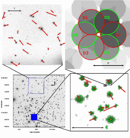
Figure 1.— The layout of a VIRUS-P observation and the quality of a guider-based astrometric solution. Bottom left: The footprints of the spectroscopic science FOV and the northernly offset guider FOV overlayed on a Digital Sky Survey (DSS) image of the open cluster M67. This type of field is used to calibrate the astrometry of the guider and the fibers as discussed in §2.3. Top left: An expanded view of the VIRUS-P guider field with residuals from the astrometric model. The residuals are shown as red vectors scaled by 60$\times$. The rms is 0$\farcs$42. Bottom right: An expanded view of the science FOV. The continuum map is generated from the IFS data summed over 4100Å$<\lambda<$5700Å. Fibers that have significant flux and border other significant fibers are highlighted with green circles and bunched as point source detections for the astrometric fit. The residuals are shown as red vectors scaled by 60$\times$. The rms is 0$\farcs$21. The residuals in the IFU are less than the residuals in the guider as both fields have a similar number of degrees of freedom, but the guider has more datapoints. Top right: The expanded view of one fiber moving through the six dither positions. The pattern, marked with D1-D6, gives very nearly an oversampling of two. The small offsets necessary to complete the dither patterns are controlled by sending offsets to the guider.

Figure 2.— Left The 5$\sigma$ detection limit under photometric conditions for an emission-line object perfectly centered in a fiber in three 20 minute exposures. Different source positions can improve or decrease this limit by $\sim$15% which is captured in our completeness calculation. In both figures, curves are given for the two focal reducers, FR1 and FR2. Right The 5$\sigma$ luminosity limit under photometric conditions for objects detected in the Ly$\alpha$ line.

Figure 3.— Left: The positional offsets from catalog emission-line detection positions and broadband counterpart image positions divided into two S/N bins. The residual correction discussed in §2.3 has been applied. The 1$\sigma$ astrometric error budget for each bin is also drawn with radii 0$\farcs$95 for $5<S/N<10$ and 0$\farcs$84 for $10<S/N<25$. Right: A histogram of the same data shown with a Rayleigh distribution. The same dispersions are used to demonstrate the appropriate characterization of the astrometric error as a two-dimensional Gaussian function.

Figure 4.— The distribution of zeropoint offsets due to non-photometric transparency as measured with the guider camera. This distribution represents the best 60${}^{\mbox{th}}$ percentile of the observing allocation with the remaining 40% being too poor to guide or requiring dome closure.

Figure 5.— The total system throughput of VIRUS-P, the 2.7m telescope, and the atmosphere at an airmass of one. Curves are given for the two eras of focal reducers, FR1 and FR2.

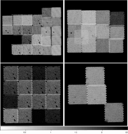
Figure 6.— Sensitivity maps (1$\sigma$ per detection element) at 4500Å in 10^-17 erg s^-1 cm^-2. The three broken fibers in fiber bundle IFU-1 are evident. Top left: COSMOS, Top right: GOODS-N, Bottom left: MUNICS, Bottom right: XMM-LSS.

Figure 7.— A histogram of the ratio between the reduced data and error for all 87.8M indepedent spectral elements in this survey. Most elements only see the sky background with residuals consistent to a normally distribution noise model. A small but obvious fraction of the elements also see bright, positive signal from continuum sources. The normalized Gaussian function shows the expected distribution in the absence of signal and systematics. The influence of the fiber throughput systematic (§3.6) likely broadens the distribution. This is most evident on the negative side which becomes nearer the normal distribution after background subtraction. The distribution after continuum subtraction appears much more symmetric and with a better matching width. The data wings at high and low ends represent the fiber positions with strong continuum. The boxcar-based continuum fitting is a rather crude tool that does not characterize all the continuum signal, but the emission line catalog is uncompromised by its use.

Figure 8.— The fractional contamination to the LAE sample by S/N cut. The detection method used is described in detail in §4.1. The LAE predictions are the same as in §2.4. Curves are given for differently sized collections of neighboring fibers. The growth of apertures was allowed whenever the S/N was increased by $>0.3$ with the inclusion of another fiber. At a high, constant S/N, the greatest contamination is produced by large apertures. The optimum sized aperture for a point source under all dither-source geometries is two at median. To optimize our selection, we make a staggered series of S/N cuts based on the number of fibers used, $N$, as S/N$>5.0+0.3\times(N-1)$. The horizontal and vertical lines show the evaluation points of this cut to the simulation curves. This procedure predicts 10%$\pm$1.6% noise contamination.

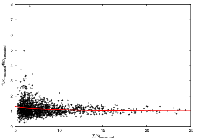
Figure 9.— The ratio of measured and input fluxes from point source simulation and a least-squares fit (§4.3). The curve-of-growth method is used here to measure emission line flux. The upturn at low S/N is expected from the Eddington bias. This ratio can be applied to the LAE flux measurements of Table 3 for some applications. The average correction is fit as flux${}_{\mbox{measured}}$/flux${}_{\mbox{true}}=$0.98+0.74/(S/N)${}_{\mbox{measured}}$+4.27/(S/N)${}_{\mbox{measured}}^{2}$

Figure 10.— The survey’s catalog completeness function for multiples of the flux limit. When combined, this function, the survey’s photometric wavelength-based flux limit in Figure 2, and the actual mosaic pattern with photometric calibration in Figure 6 define the limits necessary for volume and luminosity function calculation (Blanc et al., 2010).

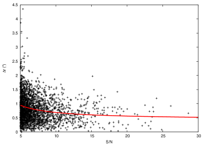
Figure 11.— The distribution of simulated source positional errors under VIRUS-P sampling patterns with a fit to the dispersion as a function of measured S/N. The maximum liklihood fit to the peak of a Rayleigh distribution gives $\sigma=0\farcs 348+2\farcs 04/(S/N)$.

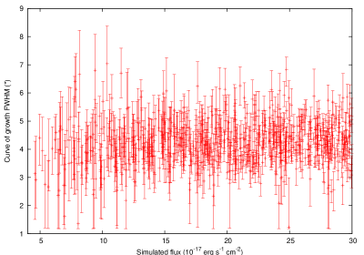
Figure 12.— The distribution of measured source sizes in simulated data. The simulation input source sizes were drawn from the survey seeing distribution. The large fiber sizes set a large resolution threshold. Based on the 99.7% confidence interval, we only claim significantly resolved measurements for curve-of-growth FWHM sizes $>6.81$″.

Figure 13.— The data, fits, and final evaluation for the curve of growth line flux measurements of a LAE (top) and an [OII] emitter (bottom). In both, the open square symbols display the cumulative sampling factor on the right hand scale. The sampling factor is written in Equation 3 as $N(\Delta r<r_{fib},r,\theta)$ and is the average number of fibers overlaying the surface enclosed in radius $r$. The points with errors show the estimated cumulative flux on the left hand scale. The vertical dotted lines mark where the fit is truncated. This threshold has been selected with consideration towards being significantly larger than the widest objects found and small enough to limit unnecessary noise. The vertical solid line marks the radius to the fit where 90% of the flux in enclosed. The horizontal solid lines show the 1$\sigma$ confidence of the fit’s normalization. The top fit returns a total flux of $24^{+3.6}_{-3.0}\times 10^{-17}$ erg s^-1 cm^-2. The bottom fit returns a total flux of $19^{+6.0}_{-4.3}\times 10^{-17}$ erg s^-1 cm^-2. The errors are correlated on the displayed scale, but the Monte Carlo fit varies the data from each fiber independently to generate proper errors.

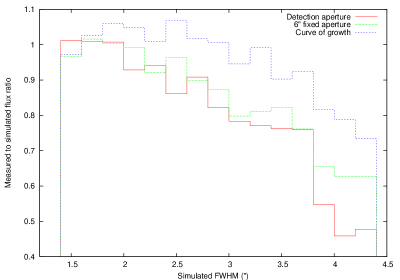
Figure 14.— Binned ratios of measured and input fluxes for simulated data under a range of source sizes. The curve-of-growth flux estimator is preferred as the least biased for extended sources compared to either the detection set of fibers or a fixed radius set of fibers as the photometry aperture.

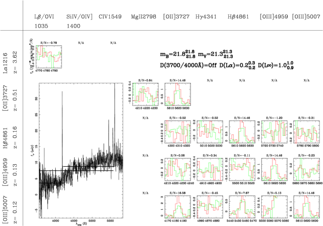
Figure 15.— The attempts to find matching lines to an [OIII]5007 detection in index 323 of Table 3. The detection is formed from two fibers represented independently with the red and green lines. The leftmost column shows the prospective identifications of our originally detected line at 5619Å. For each prospective identification, we attempt fits to the emission-line possibilities in the top row. In this case, matches to [OII] and H$\beta$ both give a clear identification. The [OIII]4959 is detected but overlapping with the mask around 5577Å. This technique only rarely gives positive evidence for Ly$\alpha$ classification by ruling out low$-z$ emission line combinations because our wavelength bandpass is not much larger than common bright optical emission-line spacings. However, is often useful in classifying transitions between low redshift options as in this case. The full spectrum is shown in the large window to the left. Various continuum regions are evaluated by assuming the primary emission line to be Ly$\alpha$ and [OII] shown by the horizontal lines. The continuum fits are used to look for various breaks as calculated in the upper right. This galaxy is also identified by significant detections of H$\beta$, [OIII]4959, and [OII] in entries 325, 326, and 327 of Table 3.

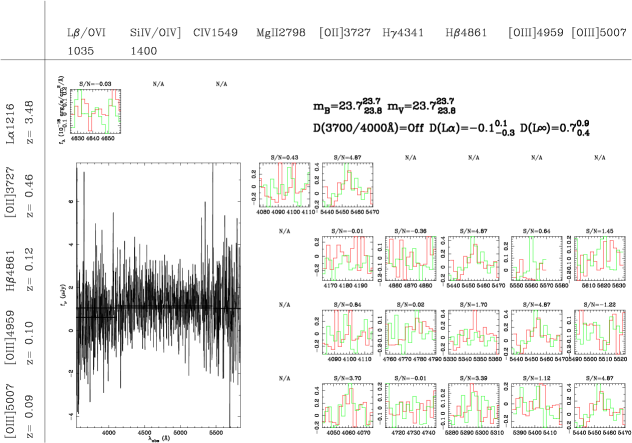
Figure 16.— The automated search for multiple emission line in index 430. The format is the same as in Figure 15. This is one of the few cases where the consideration of marginally significant counterpart lines aids the classification. The primary detection is revealed to be [OIII]5007, with marginal detections in [OII] and H$\beta$ that did not make the primary emission line catalog.

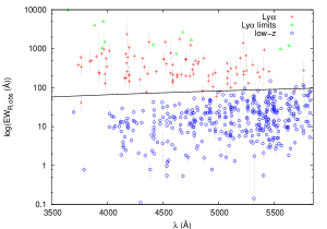
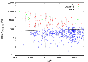
Figure 17.— The distribution of observed wavelength and observed EW. The line marks the usual EW cut used in narrowband imaging and adopted here. Exceptions to the EW selection are discussed in §5.2. Left Continuum estimated only from the $R$-band photometry (or the i’-band in MUNICS). Right Continuum estimated from interpolation with the two nearest filters bounding each emission line’s wavelength.

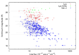
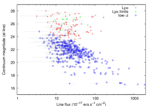
Figure 18.— The distribution of emission line flux and broadband magnitude. Left Continuum estimated only from the $R$-band photometry (or the i’-band in MUNICS). Right Continuum estimated from interpolation with the two nearest filters bounding each emission line’s wavelength.

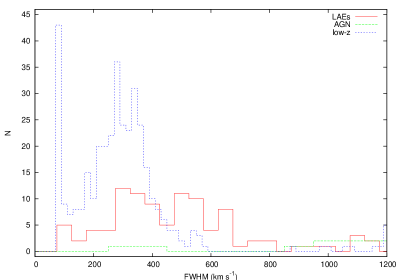
Figure 19.— The line width distributions for all survey objects. We have subtracted an instrumental resolution of 300 km s^-1 in quadrature. There is significant overlap between all populations making width-based classification impossible. No attempts have been made here to deconvolve the blended [OII] doublet. The low-$z$ objects are generally contained to low widths, but the LAE distribution overlaps heavily with both the AGN and low-$z$ distributions.

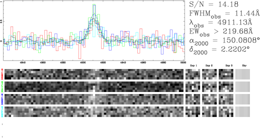
Figure 20.— The VIRUS-P emission-line detection image for index 229 which lies in the COSMOS field. This object is undoubtably a real detection with one of the largest S/N ratios we find for any high-$z$ object. In this case, the aperture is grown to include four fibers. The four rows in the Figure’s bottom half show the spectra from the four detection fibers. The right side, square cut-outs show the spectra from individual 20-minute exposures and the sky model. The three exposures in each fiber are then biweight combined into the two-dimensional, bottom-left spectra and the one-dimensional spectra in the upper-left line plot. The collapsed, one-dimensional spectra are color-coded by fiber number. The Gaussian fits to each fiber are given by dotted curves. For visual clarity, the spectra are resampled and stacked into the black histogram. Continuum is not detected within a 200Å boxcar around the line, and the high level of flux permits the Ly$\alpha$ classification from the spectrum alone in this rare case. The tabulated EW instead is based on the flux density of the imaging counterpart. The quoted central wavelength in this figure has not yet had the heliocentric and vacuum corrections applied as is done with the tabulated values.

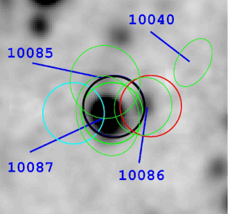
Figure 21.— The ground-based, $V_{j}$ imaging cutout for the Table 3 index 229. The four color circles represent fiber positions and are color coded in accordance with the spectra of Figure 20. The black circle indicates the emission line centroid. The Kron apertures from the imaging catalog are drawn as green, numbered ellipses. The best centered and brightest source is #10087 with an association likelihood of 87% and r⁺=23.4. The next two most likely counterparts are #10085 at 6% and r⁺=25.1 and #10087 at 5% and r⁺=24.9. Either of these would also make the LAE EW cut, and it is possible that one or more LAEs at similar redshifts are jointly contributing to the emission-line flux, but this is unlikely.

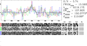
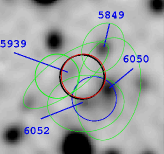
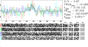
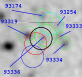
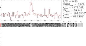
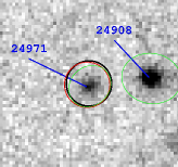
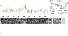
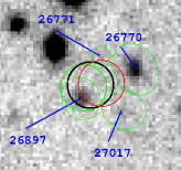
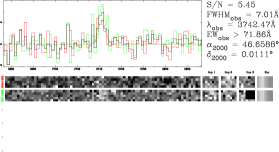
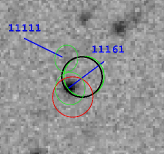
Figure 22.— Five example detections of LAEs with the same formats as Figures 20 and 21. The first two lie in the COSMOS field, the next two lie in the GOODS-N field with the first redshift previously measured and the second new, and the final one lies in the MUNICS field. The entries from Table 3 for these five are indicies 223, 160, 341, 402, and 62. The best continuum counterpart matches are to #’s 5939, 93336, 24971, 26897, and 11161.

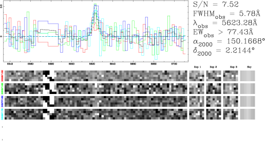
Figure 23.— The emission-line source detection for index 308 which lies in the COSMOS field. The format is the same as in Figure 20. The spectrum-based EW does not go deep enough to discriminate between the classifications. This source neither shows alternate emission lines nor has an X-ray counterpart.

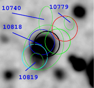
Figure 24.— The ground-based, $V_{j}$ imaging cutout for the Table 3 index 308. The detection spectra are given in Figure 23. The format is the same as in Figure 21. The counterpart #10818 at r⁺=22.1 has a 99.5% likelihood of being associated. The observed EW of $30.9_{-9.5}^{+14.9}$Å leads to a firm low-$z$ classification, presumably for [OII].

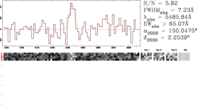
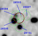
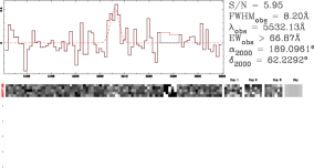
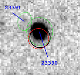
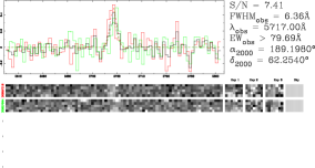
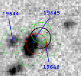
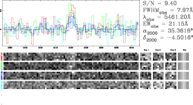
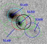
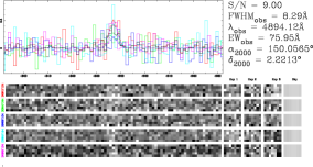
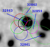
Figure 25.— Five example detections of low-$z$ objects with the format of Figure 23. The first and fifth lie in the COSMOS field, the second and third lie in the GOODS-N field both with previously measured redshifts, and the fourth lies in the XMM-LSS field. The entries from Table 3 for these five are indicies 178, 351, 406, 33, and 192. The best continuum counterpart matches are to #’s 28595, 23390, 19645, 5150, and 32863.

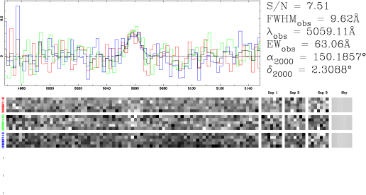
Figure 26.— The emission-line source detection for index 322 which lies in the COSMOS field. The spectrum-based EW suggests a low-$z$ classification. The format is the same as in Figure 20. Note that the emission line is broadened compared to the instrumental resolution.

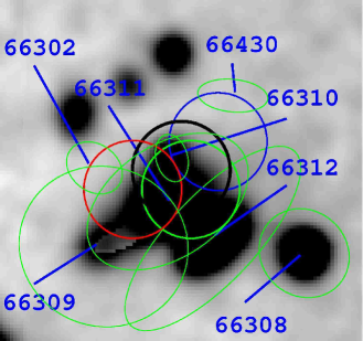
Figure 27.— The ground-based, $V_{j}$ imaging cutout for the Table 3 index 322. The detection spectra are given in Figure 26. The format is the same as in Figure 21. The counterpart #66311 at r⁺=21.1 has a 84% likelihood in association. The counterpart #66312 is already assigned to the VIRUS-P detection of Table 3 index 310 at $\lambda_{\mbox{obs}}=4948.2$Å. The counterpart #66310 at r⁺=24.9 would be a LAE based on EW and looks like a reasonable candidate system resolved from #66311 in the HST image, but it only holds a 6% chance of association. This source is associated to #66311 as an [OII] emitter in the catalog.

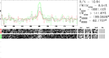
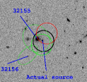
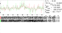
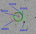
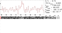
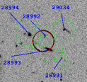
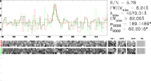
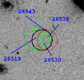
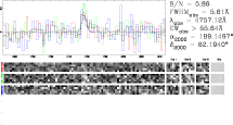
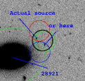
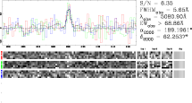
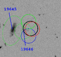
Figure 28.— The spectral detection and HST ACS F606W (Giavalisco et al., 2004) cutouts for six of the twelve new, high-$z$ redshift measurements in GOODS-N. From top to bottom, the objects are indicies 334, 338, 360, 372, 373, and 403 in Table 4. The first and fifth objects do not have identified counterparts in the ground-based images due to blending, although likely counterparts are identified in the HST data. The best counterparts for the second, third, fourth, and sixth objects are #’s 32321, 28992, 26519, and 19646.

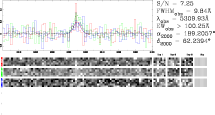
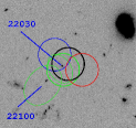
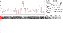
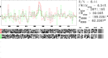
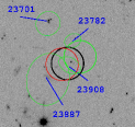
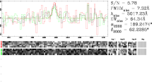
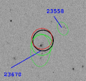
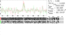
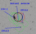
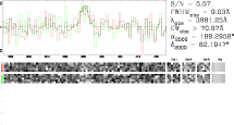
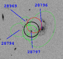
Figure 29.— The spectral detection and HST ACS F606W (Giavalisco et al., 2004) cutouts for the final six of twelve new, high-$z$ redshift measurements in GOODS-N. From top to bottom, the objects are indicies 415, 426, 434, 447, 467, and 474 in Table 4. The object with index 467 does not have an identified counterpart in the ground-based images due to blending, although a likely counterpart is identified in the HST data. The best counterparts for the remaining five, in order of listing, are 22030, 19592, 23908, 23670, and 28797.

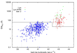
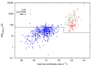
Figure 30.— The distribution of rest-frame equivalent width and line luminosity for both the LAE and low-$z$ samples. The primary classification line based on EW is drawn. The jog in the EW cut line is simply due to the cut being defined as EW${}_{\mbox{rest}}>20$Å assuming the line to be Ly$\alpha$ so the equivalent threshold in the [OII] restframe is 61Å. The drawn EW cut doesn’t strictly apply to the low-$z$ objects with emission at transitions other than [OII]. A trend between higher EW and line luminosity in the LAEs is somewhat visible but noisy over this survey’s dynamic range. The same trend is seen in surveys with lower flux limits and discussed in Cassata et al. (2010). Left Continuum estimated only from the $R$-band photometry (or the i’-band in MUNICS). Right Continuum estimated from interpolation with the two nearest filters bounding each emission line’s wavelength.

Figure 31.— The distribution of rest frame equivalent width for values with S/N$>$3 for both the LAE and low-$z$ sample by interpolating from the bounding broadband data. The LAE histogram has been scaled by 10$\times$ for visual clarity. A maximum likelihood fit was made by taking EW${}_{\mbox{rest}}>20$Å where the samples should be complete. An exponential scale length of 128$\pm$20Å fits the LAE distribution and 22$\pm$1.6Å fits the [OII] distribution. The exponential fits and error ranges are also plotted. The largest plotted bins contain all values that lie higher than the histogram range.

Figure 32.— The distribution in redshift for all the survey objects. The upper axis labels apply to the low-$z$ sample and the lower axis labels to the LAE sample. Each significantly overdense low-$z$ bin is primarily contained in one survey field. The overdensities may be early indicators of groups or clusters, but the low number statistics preclude firm classification. There are no clusters from the Koester et al. (2007b) catalog in any of this pilot survey’s area.

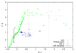
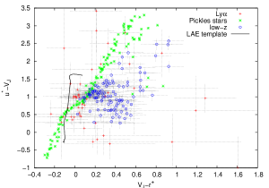
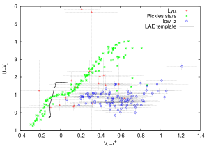
Figure 33.— Color-color plots in the photometry bands that commonly define the Lyman Break Galaxy selection. Detections are not shown for the MUNICS field where we lack $U$-band data. The LBG selection rules are sensitive to the exact filter and telescope choice, so we do not transform these filter data into systems with published LBG rules. Instead, we synthesize colors of the Gawiser et al. (2007) LAE template as the solid, black curve for $1.3<z<4.5$ and stars (Pickles, 1998). Albeit with some exceptions and frequently large color errors, the LAE sample is segregated from the low-$z$ objects and lies where expected. Top XMM-LSS objects, Middle COSMOS objects, and Bottom GOODS-N objects.

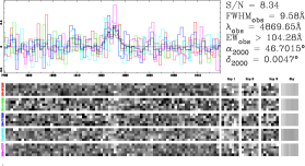
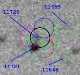
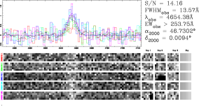
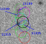
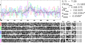
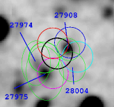
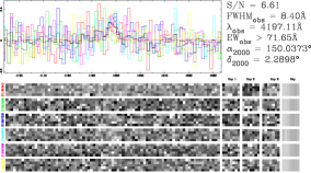
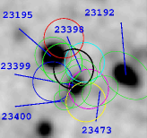
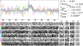
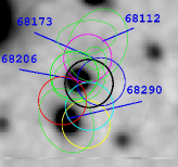
Figure 34.— The five objects significantly extended in Ly$\alpha$. Left The spectral detections. Right The $R$-band images (i’ for the first two MUNICS objects). First Index 99 in MUNICS. The best counterpart is #11720. Second Index 126 in MUNICS. The best counterpart is #11315. This source is also a high EW LAE. Third Index 162 in COSMOS. The best counterpart is #27975. This source has an X-ray detection. Fourth Index 164 in COSMOS. The best counterpart is #23399. Fifth Index 261 in COSMOS. The best counterpart is #68206. This source has an X-ray detection.

Figure 35.— The curve-of-growth plots for the five significant objects extended in Ly$\alpha$. The format is the same as in Figure 13 and described therein. Top Left Index 99 in MUNICS. The best counterpart is #11720. Top Right Index 126 in MUNICS. The best counterpart is #11315. This source is also a high EW LAE. Middle Left Index 162 in COSMOS. The best counterpart is #27975. This source has an X-ray detection. Middle Right Index 164 in COSMOS. The best counterpart is #23399. Bottom Index 261 in COSMOS. The best counterpart is #68206. This source has an X-ray detection.

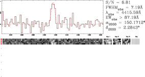
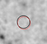
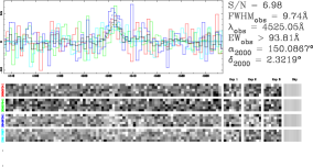
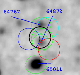
Figure 36.— The three high-significance LAEs with EW${}_{0}>$240Å. Left The spectral detection figures. Right The $R$-band images. Top Index 314 in the COSMOS field. No continuum counterpart is found. Middle Index 126 in the MUNICS field. The best counterpart is listed as #11815. The emission line is also significantly spatially extended. Bottom Index 231 in the COSMOS field. The best counterpart is listed as #64872.

Table 1Summary of VIRUS-P Observations

Date	Number of	Fields	Median	Range of	Number of
	pointings		A${}_{\mbox{V}}$ used	A${}_{\mbox{V}}$ used	emission line
					detections
2007 Oct 04-09	3	MUNICS S2	0.29	0.18-0.44	21
2007 Nov 05-10	5	MUNICS S2;COSMOS	0.33	0.00-1.48	26
2007 Dec 04-09	6	MUNICS S2;COSMOS	0.24	0.23-0.42	36
2008 Jan 03-10	8	MUNICS S2;COSMOS	0.25	0.00-2.84	71
2008 Feb 01-12	6	MUNICS S2;COSMOS;GOODS-N	0.28	0.00-1.63	27
2008 Apr 01-07	3	COSMOS;GOODS-N	0.30	0.00-0.97	30
2008 Apr 28-May 03	3	GOODS-N	0.39	0.00-2.77	43
2008 Jun 03-09	2	GOODS-N	0.31	0.00-1.69	0
2008 Sep 24-29	2	XMM-LSS	0.36	0.19-0.51	28
2008 Nov 24-30	2	COSMOS	0.13	0.07-0.46	8
2008 Dec 22-27	4	COSMOS;XMM-LSS	0.23	0.13-0.47	40
2009 Jan 21-27	3	COSMOS;XMM-LSS	0.23	0.13-0.67	46
2009 Feb 19-23	4	COSMOS;GOODS-N	0.19	0.00-0.53	27
2009 Mar 20-25	4	COSMOS;GOODS-N	0.34	0.00-0.92	29
2009 Apr 20-25	2	GOODS-N	0.20	0.07-0.48	28
2009 May 20-25	1	GOODS-N	0.21	0.00-1.55	5
2010 Feb 09-11	1	COSMOS	0.30	0.10-0.50	0

Table 2Ancillary broadband imaging properties

Field	Central $\alpha$	Central $\delta$	E(B-V)	Filters	FWHM	Stack	BandK	Depth	VIRUS-P
	(J2000)	(J2000)							area (□′)
COSMOS	10:00:30	+02:15:04	0.018	u*,BJ,VJ,r’,i’,z’	1.33	BJr’i’	VJ	26.5	71.6
GOODS-N	12:36:51	+62:12:51	0.012	UJ,BJ,VJ,RJ,IJ,z’	1.26	BJRJI	VJ	26.6	35.5
MUNICS-S2	03:06:41	+00:01:15	0.083	BJ,g’,i’,z’	0.99	BJg’i’	g’	25.8	49.9
XMM-LSS	02:21:20	-04:30:00	0.027	u*,g’,r’,i’,z’	0.97	g’r’i’	g’	25.8	12.3

Table 3HETDEX Pilot Survey Emission Line Catalog (Abridged)

HPS Index	$\alpha$	$\delta$	$\lambda_{\mbox{det}}$	FWHM	S/N${}_{\mbox{det}}$	Flux	Spatial	Matching
	(J2000)	(J2000)	(Å)	(km s-1)		(10-17 cgs)	FWHM (″)	indices
(1)	(2)	(3)	(4)	(5)	(6)	(7)	(8)	(9)
001	02:21:11.16	-04:31:25.0	5219.16	229	8.1	17.4${}_{-3.9}^{3.5}$	4.7${}_{-0.6}^{0.8}$	..
002	02:21:12.21	-04:32:25.3	5448.72	307	5.6	12.2${}_{-4.3}^{3.6}$	4.3${}_{-1.0}^{0.8}$	..
003	02:21:14.28	-04:31:38.2	4973.93	422	7.5	19.9${}_{-3.1}^{4.7}$	4.4${}_{-0.5}^{0.8}$	..
004	02:21:14.86	-04:31:56.6	5261.37	1285	6.3	42.6${}_{-12.4}^{11.2}$	5.1${}_{-0.9}^{0.7}$	5
005	02:21:15.14	-04:31:54.0	4270.67	1841	33.1	342.1${}_{-14.3}^{16.5}$	4.8${}_{-0.1}^{0.2}$	4
006	02:21:16.26	-04:29:32.8	4591.58	399	14.8	32.7${}_{-3.6}^{3.5}$	4.6${}_{-0.2}^{0.4}$	..
007	02:21:16.35	-04:31:14.6	5161.72	293	19.5	49.4${}_{-4.4}^{2.6}$	4.7${}_{-0.2}^{0.2}$	..
008	02:21:17.25	-04:27:55.7	5820.13	118	6.7	19.1${}_{-3.2}^{5.0}$	6.6${}_{-0.6}^{0.9}$	..
009	02:21:17.25	-04:30:10.4	5464.33	78	12.1	14.1${}_{-2.5}^{1.5}$	3.6${}_{-0.4}^{0.5}$	..
010	02:21:17.47	-04:27:30.6	4808.33	357	15.9	38.9${}_{-3.6}^{3.4}$	4.6${}_{-0.3}^{0.2}$	..
011	02:21:18.48	-04:27:32.2	4590.82	441	6.6	21.2${}_{-4.6}^{4.7}$	5.9${}_{-0.7}^{0.7}$	..
012	02:21:19.20	-04:30:28.9	4398.59	344	9.9	26.4${}_{-3.9}^{4.0}$	5.7${}_{-0.5}^{0.6}$	..
013	02:21:19.22	-04:30:39.9	5250.96	378	7.8	11.7${}_{-1.9}^{2.6}$	3.6${}_{-0.5}^{0.7}$	..
014	02:21:19.47	-04:28:21.9	4863.62	328	21.8	49.6${}_{-3.8}^{2.4}$	5.5${}_{-0.2}^{0.2}$	..
015	02:21:19.48	-04:29:34.0	4919.31	243	21.7	36.2${}_{-2.8}^{2.8}$	4.9${}_{-0.3}^{0.2}$	..
016	02:21:19.83	-04:28:08.8	4901.07	397	5.9	13.7${}_{-3.1}^{5.2}$	5.3${}_{-1.2}^{1.2}$	..
017	02:21:19.85	-04:27:43.4	4588.13	93	5.9	13.2${}_{-3.4}^{3.9}$	5.3${}_{-0.9}^{1.1}$	..
018	02:21:20.77	-04:30:56.6	5655.44	972	8.2	45.4${}_{-7.5}^{8.4}$	5.6${}_{-0.6}^{0.4}$	19
019	02:21:20.78	-04:30:56.4	5452.07	438	26.8	83.6${}_{-4.0}^{4.2}$	5.6${}_{-0.1}^{0.1}$	18
020	02:21:21.27	-04:27:44.6	5788.83	303	8.9	21.8${}_{-3.9}^{3.9}$	5.1${}_{-0.6}^{0.8}$	..
021	02:21:22.13	-04:30:35.0	5448.33	277	8.6	8.8${}_{-1.9}^{2.4}$	3.3${}_{-0.8}^{0.7}$	..
022	02:21:22.84	-04:29:25.2	4586.30	603	7.4	17.7${}_{-4.3}^{5.5}$	5.2${}_{-0.9}^{0.8}$	..
023	02:21:22.88	-04:29:44.3	4540.36	323	9.4	18.5${}_{-4.1}^{3.2}$	4.6${}_{-0.6}^{0.7}$	..
024	02:21:23.28	-04:29:22.3	4592.57	204	8.8	14.3${}_{-2.5}^{3.7}$	4.0${}_{-0.5}^{0.6}$	..
…
033	02:21:26.83	-04:30:05.8	5460.20	343	9.4	25.4${}_{-4.6}^{3.6}$	5.0${}_{-0.6}^{0.5}$	..
051	03:06:34.61	-00:00:49.6	4980.74	428	5.2	9.1${}_{-4.0}^{5.0}$	3.5${}_{-1.7}^{1.4}$	..
062	03:06:38.12	+00:00:40.0	3741.83	392	5.5	67.7${}_{-21.0}^{22.9}$	3.4${}_{-1.0}^{1.3}$	..
085	03:06:41.48	+00:01:10.8	3699.08	2323	7.5	288.3${}_{-59.8}^{90.6}$	3.5${}_{-0.7}^{0.7}$	86
092	03:06:44.44	+00:01:46.7	5682.19	363	6.0	13.2${}_{-4.3}^{4.2}$	4.4${}_{-0.7}^{1.0}$	..
094	03:06:46.23	+00:02:18.3	5767.11	370	22.7	134.7${}_{-11.4}^{9.6}$	6.0${}_{-0.4}^{0.2}$	..
099	03:06:48.36	+00:00:17.0	4868.35	505	8.3	33.0${}_{-5.3}^{8.3}$	7.4${}_{-0.6}^{0.7}$	..
126	03:06:55.26	+00:00:33.8	4653.11	815	14.2	167.1${}_{-13.8}^{14.8}$	7.5${}_{-0.3}^{0.5}$	..
160	10:00:08.61	+02:17:38.6	4175.32	663	6.0	17.1${}_{-6.4}^{10.5}$	5.2${}_{-1.6}^{1.5}$	..
162	10:00:08.73	+02:15:32.0	4167.83	1063	7.3	76.4${}_{-11.5}^{14.6}$	8.3${}_{-0.9}^{1.3}$	..
164	10:00:08.95	+02:17:23.2	4196.31	482	6.6	25.4${}_{-12.9}^{13.7}$	11.0${}_{-3.3}^{3.3}$	..
178	10:00:11.39	+02:15:14.1	5484.87	283	5.8	10.1${}_{-2.6}^{3.5}$	4.8${}_{-0.7}^{0.8}$	..
192	10:00:13.57	+02:13:16.6	4893.46	406	9.0	23.6${}_{-4.9}^{3.9}$	5.4${}_{-0.6}^{0.6}$	..
223	10:00:18.56	+02:14:59.8	4018.61	1102	5.7	39.0${}_{-9.4}^{11.5}$	6.4${}_{-0.9}^{1.0}$	..
229	10:00:19.39	+02:13:12.6	4910.43	625	14.2	41.6${}_{-5.0}^{4.2}$	5.4${}_{-0.3}^{0.5}$	..
231	10:00:20.80	+02:19:18.8	4524.17	551	7.0	30.8${}_{-7.6}^{8.0}$	6.3${}_{-0.7}^{1.1}$	..
234	10:00:21.49	+02:13:51.5	5465.91	78	14.1	24.4${}_{-3.0}^{3.6}$	4.5${}_{-0.4}^{0.4}$	..
261	10:00:28.57	+02:17:48.4	3763.70	886	9.8	143.7${}_{-10.1}^{23.2}$	8.3${}_{-0.6}^{0.9}$	..
289	10:00:35.24	+02:18:07.3	5235.12	428	6.4	17.1${}_{-4.5}^{4.5}$	6.5${}_{-1.3}^{1.2}$	..
308	10:00:40.04	+02:12:51.7	5622.45	157	7.5	18.4${}_{-4.2}^{3.5}$	5.4${}_{-0.9}^{0.8}$	..
310	10:00:40.70	+02:17:41.5	4948.20	532	7.7	10.7${}_{-2.4}^{2.9}$	4.0${}_{-0.6}^{0.7}$	..
313	10:00:40.78	+02:18:23.6	3765.58	249	5.9	25.1${}_{-10.1}^{12.4}$	5.0${}_{-1.3}^{1.8}$	..
314	10:00:41.09	+02:17:03.6	4414.31	352	6.8	14.4${}_{-2.9}^{5.7}$	3.7${}_{-0.7}^{1.1}$	..
322	10:00:44.57	+02:18:31.6	5057.65	486	7.5	16.7${}_{-3.3}^{4.4}$	4.7${}_{-0.8}^{0.9}$	..
323	10:00:45.12	+02:18:22.0	5617.75	213	15.3	36.7${}_{-2.8}^{3.9}$	5.1${}_{-0.3}^{0.4}$	324,325,326
341	12:36:17.52	+62:13:10.0	4778.04	298	9.3	12.8${}_{-2.8}^{4.1}$	3.8${}_{-0.6}^{0.8}$	..
351	12:36:23.05	+62:13:45.0	5530.63	352	6.0	33.7${}_{-12.1}^{13.8}$	7.1${}_{-1.4}^{1.5}$	..
356	12:36:29.24	+62:11:53.4	5698.97	315	9.0	25.6${}_{-6.1}^{7.2}$	7.1${}_{-0.7}^{1.0}$	..
371	12:36:35.34	+62:14:23.4	4660.93	957	6.0	13.9${}_{-5.5}^{4.1}$	3.7${}_{-1.4}^{1.1}$	..
400	12:36:46.37	+62:14:08.4	5651.77	76	7.2	5.9${}_{-2.0}^{1.7}$	2.5${}_{-1.4}^{1.0}$	..
402	12:36:46.86	+62:12:27.4	4821.05	630	8.3	16.8${}_{-3.2}^{1.7}$	3.9${}_{-0.5}^{0.5}$	..
406	12:36:47.53	+62:15:14.3	5715.47	209	7.4	10.6${}_{-2.3}^{1.2}$	4.1${}_{-0.7}^{0.8}$	..
430	12:36:52.03	+62:11:25.9	5452.19	79	5.9	6.6${}_{-1.9}^{2.3}$	4.3${}_{-1.2}^{1.1}$	..
439	12:36:56.87	+62:11:52.0	5760.95	232	6.5	8.4${}_{-2.6}^{3.0}$	4.2${}_{-0.9}^{1.2}$	..
447	12:36:59.37	+62:13:42.6	5016.05	318	5.8	7.2${}_{-1.2}^{2.1}$	4.4${}_{-0.9}^{0.9}$	..

Note. — Table 3 is published in its entirety in the electronic edition of the ApJS. A portion is shown here to display its form and content.

Table 4HETDEX Pilot Survey Emission Line Classifications (Abridged)

HPS Index	Counter-	Counter-	Counter-	EW${}_{\mbox{R,rest}}$	EW${}_{\mbox{interp,rest}}$	Trans-	$z_{\mbox{est}}$	Ly$\alpha$	X-ray
	part	part m${}_{\mbox{R}}$	part P	(Å)	(Å)	ition		P	counterpart
(1)	(2)	(3)	(4)	(5)	(6)	(7)	(8)	(9)	(10)
001	J0221112-043126	23.05	0.93	51.9${}_{-14.6}^{14.7}$	62.9${}_{-17.4}^{17.0}$	[OII]	0.4004	0.07	..
002	J0221122-043225	23.17	0.96	42.0${}_{-16.3}^{14.9}$	59.8${}_{-23.0}^{20.5}$	[OII]	0.4620	0.04	..
003	J0221143-043138	24.31	0.98	58.8${}_{-15.1}^{22.2}$	109.0${}_{-26.5}^{36.8}$	Ly$\alpha$	3.0915	1.00	..
004	J0221150-043156	21.05	0.98	10.4${}_{-3.5}^{3.4}$	7.1${}_{-2.4}^{2.3}$	CIII]1909	1.7561	0.02	J0221151-043156
005	J0221150-043156	21.05	1.00	54.9${}_{-9.7}^{10.9}$	55.1${}_{-9.2}^{9.9}$	CIV1549	1.7570	0.00	J0221151-043156
006	J0221164-042933	23.82	0.89	56.7${}_{-11.5}^{12.6}$	74.1${}_{-14.8}^{15.8}$	Ly$\alpha$	2.7770	1.00	..
007	J0221163-043116	21.38	0.98	31.2${}_{-6.0}^{6.2}$	48.3${}_{-8.9}^{8.8}$	[OII]	0.3850	0.02	..
008	J0221171-042757	22.82	0.67	51.2${}_{-12.1}^{16.8}$	57.4${}_{-13.3}^{18.3}$	[OII]	0.5616	0.01	..
009	J0221174-043001	23.21	0.98	51.0${}_{-12.4}^{11.2}$	49.0${}_{-11.6}^{9.9}$	[OII]	0.4661	0.02	..
010	J0221174-042729	21.43	0.99	24.0${}_{-4.6}^{5.1}$	39.1${}_{-7.5}^{8.2}$	[OII]	0.2901	0.01	..
011	J0221185-042734	23.93	0.56	40.8${}_{-11.1}^{12.2}$	39.3${}_{-10.6}^{11.3}$	Ly$\alpha$	2.7764	1.00	..
012	J0221194-043029	20.27	1.00	5.1${}_{-1.1}^{1.3}$	14.3${}_{-3.1}^{3.4}$	[OII]	0.1802	0.00	..
013	J0221193-043039	24.91	0.70	62.9${}_{-17.5}^{26.5}$	92.3${}_{-23.3}^{31.4}$	Ly$\alpha$	3.3194	1.00	..
014	J0221194-042822	21.69	1.00	39.3${}_{-7.3}^{7.8}$	55.5${}_{-10.3}^{10.9}$	[OII]	0.3050	0.00	..
015	J0221196-042934	20.62	1.00	10.7${}_{-2.0}^{2.2}$	18.8${}_{-3.5}^{3.8}$	[OII]	0.3199	0.00	..
016	J0221198-042801	22.17	0.84	17.0${}_{-4.8}^{7.3}$	25.8${}_{-7.2}^{11.1}$	[OII]	0.3150	0.00	..
017	J0221199-042743	24.33	0.96	36.4${}_{-11.3}^{13.7}$	34.2${}_{-10.4}^{12.0}$	Ly$\alpha$	2.7742	1.00	..
018	J0221208-043057	20.49	0.74	14.4${}_{-3.4}^{3.9}$	20.4${}_{-4.7}^{5.3}$	[NeIII]3869	0.4617	0.00	..
019	J0221208-043057	20.48	0.75	24.3${}_{-4.3}^{4.8}$	41.1${}_{-7.0}^{7.5}$	[OII]	0.4629	0.00	..
020	J0221211-042744	21.80	0.99	22.7${}_{-5.6}^{6.0}$	27.0${}_{-6.6}^{6.9}$	[OII]	0.5532	0.01	..
021	J0221223-043034	23.13	0.60	29.5${}_{-7.9}^{10.1}$	40.2${}_{-10.6}^{13.2}$	[OII]	0.4619	0.03	..
022	J0221230-042925	25.14	0.81	103.4${}_{-42.9}^{122.1}$	682.6${}_{-328.6}^{1000.0}$	Ly$\alpha$	2.7727	1.00	..
023	J0221229-042944	22.44	1.00	27.1${}_{-7.5}^{7.1}$	44.1${}_{-12.1}^{11.1}$	[OII]	0.2182	0.00	..
024	J0221233-042923	22.03	1.00	14.6${}_{-3.5}^{4.8}$	21.2${}_{-5.0}^{6.8}$	[OII]	0.2322	0.00	..
…
033	J0221269-043006	22.59	0.54	51.6${}_{-12.7}^{12.4}$	69.2${}_{-16.6}^{15.5}$	[OII]	0.4650	0.01	..
051	J0306348-000051	23.67	0.47	14.8${}_{-7.0}^{9.3}$	26.3${}_{-12.3}^{15.5}$	Ly$\alpha$	3.0971	0.52	..
062	J0306382+000039	24.11	0.95	125.3${}_{-44.5}^{52.1}$	205.9${}_{-73.0}^{84.9}$	Ly$\alpha$	2.0780	1.00	..
085	J0306417+000108	19.53	0.99	17.8${}_{-4.7}^{6.6}$	37.1${}_{-9.9}^{13.9}$	MgII2798	0.3220	0.01	J0306417+000109
092	J0306444+000146	23.33	0.98	18.0${}_{-6.6}^{7.2}$	29.7${}_{-10.8}^{11.1}$	Ly$\alpha$	3.6741	1.00	..
094	J0306463+000219	21.03	0.99	68.9${}_{-13.1}^{14.1}$	105.9${}_{-19.3}^{19.7}$	[OII]	0.5474	0.01	..
099	J0306484+000017	24.75	0.55	142.8${}_{-39.7}^{63.9}$	401.3${}_{-114.5}^{190.1}$	Ly$\alpha$	3.0047	1.00	..
126	J0306554+000033	24.31	0.77	461.7${}_{-109.9}^{156.3}$	5461.0${}_{-2730.5}^{1000.0}$	Ly$\alpha$	2.8276	1.00	..
160	J1000086+021739	27.35	0.61	698.3${}_{-333.5}^{1000.0}$	1034.3${}_{-559.0}^{1000.0}$	Ly$\alpha$	2.4346	1.00	..
162	J1000088+021529	24.45	0.20	214.4${}_{-39.0}^{52.8}$	564.3${}_{-114.8}^{165.4}$	Ly$\alpha$	2.4284	1.00	J100008.8+021528
164	J1000089+021721	24.32	0.31	63.3${}_{-32.3}^{35.6}$	126.4${}_{-64.5}^{70.5}$	Ly$\alpha$	2.4518	1.00	..
178	J1000115+021513	23.27	0.64	38.5${}_{-10.4}^{14.4}$	59.7${}_{-16.1}^{22.3}$	[OII]	0.4717	0.36	..
192	J1000135+021317	22.02	0.99	25.3${}_{-5.6}^{5.2}$	44.1${}_{-9.4}^{8.2}$	[OII]	0.3130	0.01	..
223	J1000187+021460	25.46	0.31	268.2${}_{-86.7}^{157.1}$	1919.9${}_{-959.9}^{1000.0}$	Ly$\alpha$	2.3057	1.00	..
229	J1000194+021312	23.37	0.87	50.7${}_{-7.5}^{7.8}$	71.3${}_{-9.6}^{9.2}$	Ly$\alpha$	3.0393	1.00	..
231	J1000208+021918	26.02	0.74	400.3${}_{-118.3}^{168.7}$	1633.7${}_{-816.9}^{1000.0}$	Ly$\alpha$	2.7215	1.00	..
234	J1000215+021350	23.37	0.63	136.8${}_{-20.6}^{26.0}$	133.8${}_{-20.1}^{25.4}$	[OIII]5007	0.0917	0.37	..
261	J1000286+021749	23.76	0.87	193.4${}_{-21.9}^{38.9}$	536.7${}_{-92.4}^{157.8}$	Ly$\alpha$	2.0960	1.00	J100028.6+021745
289	J1000351+021806	23.37	0.63	68.4${}_{-18.7}^{20.2}$	146.0${}_{-39.6}^{41.9}$	[OII]	0.4046	0.37	..
308	J1000401+021251	22.11	1.00	24.8${}_{-6.0}^{5.6}$	26.6${}_{-6.4}^{5.7}$	[OII]	0.5086	0.00	..
310	J1000407+021741	24.92	0.72	54.7${}_{-13.7}^{18.7}$	79.5${}_{-18.6}^{24.0}$	Ly$\alpha$	3.0703	0.98	..
313	J1000408+021823	22.75	0.98	13.4${}_{-5.4}^{6.9}$	23.9${}_{-9.7}^{12.3}$	Ly$\alpha$	2.0975	1.00	..
314	..	..	0.97	435.4${}_{-87.7}^{173.4}$	435.4${}_{-87.7}^{173.4}$	Ly$\alpha$	2.6312	1.00	..
322	J1000446+021830	21.14	0.84	8.2${}_{-1.8}^{2.4}$	27.9${}_{-5.8}^{8.0}$	[OII]	0.3570	0.08	..
323	J1000453+021822	19.88	0.89	8.5${}_{-1.0}^{1.3}$	9.9${}_{-1.0}^{1.4}$	[OIII]5007	0.1220	0.11	..
341	J1236175+621301	24.81	0.97	57.1${}_{-14.6}^{23.4}$	87.1${}_{-22.8}^{37.3}$	Ly$\alpha$	2.9304	1.00	..
351	J1236231+621346	21.10	1.00	17.5${}_{-6.4}^{7.6}$	33.2${}_{-12.0}^{14.2}$	[OII]	0.4839	0.00	J1236230+621347
356	J1236292+621153	22.84	0.98	68.2${}_{-16.9}^{21.1}$	106.6${}_{-25.9}^{31.4}$	[OII]	0.5291	0.02	..
371	J1236356+621424	23.45	0.36	22.2${}_{-9.0}^{7.1}$	30.5${}_{-12.3}^{9.7}$	CIV1549	2.0090	0.27	J1236356+621424
400	J1236465+621408	23.75	0.59	48.1${}_{-16.9}^{15.3}$	50.2${}_{-17.6}^{15.4}$	[OIII]	0.1290	0.01	J1236463+621405
402	J1236470+621226	25.27	0.43	115.5${}_{-29.2}^{35.8}$	220.0${}_{-65.2}^{108.5}$	Ly$\alpha$	2.9658	1.00	..
406	J1236478+621513	21.69	0.90	9.9${}_{-2.3}^{1.6}$	15.9${}_{-3.6}^{2.2}$	[OII]	0.5335	0.10	..
430	J1236519+621125	21.88	1.00	9.3${}_{-2.7}^{3.4}$	11.5${}_{-3.3}^{4.2}$	[OIII]5007	0.0889	0.00	..
439	J1236573+621153	24.17	0.54	77.0${}_{-25.3}^{33.4}$	92.5${}_{-29.0}^{34.8}$	[OII]	0.5457	0.46	..
447	J1236595+621341	24.22	0.93	19.7${}_{-4.3}^{7.5}$	31.3${}_{-5.9}^{10.1}$	Ly$\alpha$	3.1262	1.00	..

Note. — Table 4 is published in its entirety in the electronic edition of the ApJS. A portion is shown here to display its form and content.

Table 5Emission line/X-ray counterpart statistics

Field	Low-z counterparts	High-z counterparts	Depth
COSMOS	2/112	4/55	0.73
GOODS-N	27/94	2/25	0.14
XMM-LSS	1/24	0/8	$\sim$27
MUNICS	4/63	0/16	$\sim$20

References

- Adams et al. (2008) Adams, J. J., Hill, G. J., & MacQueen, P. J. 2008, in Society of Photo-Optical Instrumentation Engineers (SPIE) Conference Series, Vol. 7014, 232
- Adelman-McCarthy et al. (2008) Adelman-McCarthy, J. K., et al. 2008, ApJS, 175, 297
- Alexander et al. (2003) Alexander, D. M., et al. 2003, AJ, 126, 539
- Allen (1973) Allen, C. W. 1973, Astrophysical quantities, ed. Allen, C. W.
- Barden et al. (1998) Barden, S. C., Sawyer, D. G., & Honeycutt, R. K. 1998, in Presented at the Society of Photo-Optical Instrumentation Engineers (SPIE) Conference, Vol. 3355, Society of Photo-Optical Instrumentation Engineers (SPIE) Conference Series, ed. S. D’Odorico, 892–899
- Barger et al. (2008) Barger, A. J., Cowie, L. L., & Wang, W. 2008, ApJ, 689, 687
- Becker (2002) Becker, T. 2002
- Beers et al. (1990) Beers, T. C., Flynn, K., & Gebhardt, K. 1990, AJ, 100, 32
- Bertin & Arnouts (1996) Bertin, E., & Arnouts, S. 1996, A&AS, 117, 393
- Blanc et al. (2010) Blanc, G., et al. 2010, ApJ, in prep.
- Bond et al. (2010) Bond, N. A., Feldmeier, J. J., Matković, A., Gronwall, C., Ciardullo, R., & Gawiser, E. 2010, ApJ, 716, L200
- Bongiovanni et al. (2010) Bongiovanni, É., et al. 2010, A&A, 519, L4+
- Bower et al. (2004) Bower, R. G., Morris, S. L., Bacon, R., Wilman, R. J., Sullivan, M., Chapman, S., Davies, R. L., de Zeeuw, P. T., & Emsellem, E. 2004, MNRAS, 351, 63
- Brammer et al. (2008) Brammer, G. B., van Dokkum, P. G., & Coppi, P. 2008, ApJ, 686, 1503
- Capak et al. (2004) Capak, P., et al. 2004, AJ, 127, 180
- Capak et al. (2007) —. 2007, ApJS, 172, 99
- Cappelluti et al. (2007) Cappelluti, N., et al. 2007, ApJS, 172, 341
- Cappelluti et al. (2009) —. 2009, A&A, 497, 635
- Cassata et al. (2010) Cassata, P., et al. 2010, ArXiv e-prints
- Charlot & Fall (1993) Charlot, S., & Fall, S. M. 1993, ApJ, 415, 580
- Cowie & Hu (1998) Cowie, L. L., & Hu, E. M. 1998, AJ, 115, 1319
- Daddi et al. (2004) Daddi, E., Cimatti, A., Renzini, A., Fontana, A., Mignoli, M., Pozzetti, L., Tozzi, P., & Zamorani, G. 2004, ApJ, 617, 746
- Dickinson et al. (2003) Dickinson, M., Giavalisco, M., & GOODS Team. 2003, in The Mass of Galaxies at Low and High Redshift, ed. R. Bender & A. Renzini, 324–+
- Dierckx (1993) Dierckx, P. 1993, Curve and surface fitting with splines (Monographs on Numerical Analysis, Oxford: Clarendon, —c1993)
- Drory et al. (2001) Drory, N., Feulner, G., Bender, R., Botzler, C. S., Hopp, U., Maraston, C., Mendes de Oliveira, C., & Snigula, J. 2001, MNRAS, 325, 550
- Eddington (1913) Eddington, A. S. 1913, MNRAS, 73, 359
- Eddington (1940) Eddington, Sir, A. S. 1940, MNRAS, 100, 354
- Elvis et al. (2009) Elvis, M., et al. 2009, ApJS, 184, 158
- Fernández-Soto et al. (1999) Fernández-Soto, A., Lanzetta, K. M., & Yahil, A. 1999, ApJ, 513, 34
- Filippenko (1982) Filippenko, A. V. 1982, PASP, 94, 715
- Finkelstein et al. (2009) Finkelstein, S. L., Rhoads, J. E., Malhotra, S., & Grogin, N. 2009, ApJ, 691, 465
- Francis et al. (2001) Francis, P. J., et al. 2001, ApJ, 554, 1001
- Furusawa et al. (2008) Furusawa, H., et al. 2008, ApJS, 176, 1
- Gallego et al. (2002) Gallego, J., García-Dabó, C. E., Zamorano, J., Aragón-Salamanca, A., & Rego, M. 2002, ApJ, 570, L1
- Gawiser et al. (2006) Gawiser, E., et al. 2006, ApJ, 642, L13
- Gawiser et al. (2007) —. 2007, ApJ, 671, 278
- Giavalisco et al. (2004) Giavalisco, M., et al. 2004, ApJ, 600, L93
- Gilbank et al. (2010) Gilbank, D. G., Balogh, M. L., Glazebrook, K., Bower, R. G., Baldry, I. K., Davies, G. T., Hau, G. K. T., Li, I. H., & McCarthy, P. 2010, MNRAS, 405, 2419
- Greisen & Calabretta (1993) Greisen, E. W., & Calabretta, M. 1993, in Bulletin of the American Astronomical Society, Vol. 25, Bulletin of the American Astronomical Society, 808–+
- Gronwall et al. (2007) Gronwall, C., et al. 2007, ApJ, 667, 79
- Guaita et al. (2010) Guaita, L., et al. 2010, ApJ, 714, 255
- Hammer et al. (1997) Hammer, F., Flores, H., Lilly, S. J., Crampton, D., Le Fevre, O., Rola, C., Mallen-Ornelas, G., Schade, D., & Tresse, L. 1997, ApJ, 481, 49
- Hayashino et al. (2004) Hayashino, T., et al. 2004, AJ, 128, 2073
- Hill et al. (2004) Hill, G. J., Gebhardt, K., Komatsu, E., & MacQueen, P. J. 2004, in American Institute of Physics Conference Series, Vol. 743, The New Cosmology: Conference on Strings and Cosmology, ed. R. E. Allen, D. V. Nanopoulos, & C. N. Pope, 224–233
- Hill et al. (2008a) Hill, G. J., et al. 2008a, in Astronomical Society of the Pacific Conference Series, Vol. 399, Astronomical Society of the Pacific Conference Series, ed. T. Kodama, T. Yamada, & K. Aoki, 115–+
- Hill et al. (2008b) Hill, G. J., et al. 2008b, in Society of Photo-Optical Instrumentation Engineers (SPIE) Conference Series, Vol. 7014, 231
- Hill et al. (2010) Hill, G. J., et al. 2010, in Society of Photo-Optical Instrumentation Engineers (SPIE) Conference Series, Vol. 7735, 21
- Hogg et al. (1998) Hogg, D. W., Cohen, J. G., Blandford, R., & Pahre, M. A. 1998, ApJ, 504, 622
- Hu et al. (2004) Hu, E. M., Cowie, L. L., Capak, P., McMahon, R. G., Hayashino, T., & Komiyama, Y. 2004, AJ, 127, 563
- Hu et al. (2009) Hu, E. M., Cowie, L. L., Kakazu, Y., & Barger, A. J. 2009, ApJ, 698, 2014
- Hu & McMahon (1996) Hu, E. M., & McMahon, R. G. 1996, Nature, 382, 231
- Ilbert et al. (2009) Ilbert, O., et al. 2009, ApJ, 690, 1236
- Jeong & Komatsu (2006) Jeong, D., & Komatsu, E. 2006, ApJ, 651, 619
- Jeong & Komatsu (2009) —. 2009, ApJ, 691, 569
- Kakazu et al. (2007) Kakazu, Y., Cowie, L. L., & Hu, E. M. 2007, ApJ, 668, 853
- Kelson (2003) Kelson, D. D. 2003, PASP, 115, 688
- Kennicutt (1992) Kennicutt, Jr., R. C. 1992, ApJ, 388, 310
- Koehler et al. (2007) Koehler, R. S., Schuecker, P., & Gebhardt, K. 2007, A&A, 462, 7
- Koester et al. (2007a) Koester, B. P., et al. 2007a, ApJ, 660, 239
- Koester et al. (2007b) —. 2007b, ApJ, 660, 239
- Kornei et al. (2010) Kornei, K. A., Shapley, A. E., Erb, D. K., Steidel, C. C., Reddy, N. A., Pettini, M., & Bogosavljević, M. 2010, ApJ, 711, 693
- Kron (1980) Kron, R. G. 1980, ApJS, 43, 305
- Kurtz & Mink (1998) Kurtz, M. J., & Mink, D. J. 1998, PASP, 110, 934
- Lemaux et al. (2009) Lemaux, B. C., Lubin, L. M., Sawicki, M., Martin, C., Lagattuta, D. J., Gal, R. R., Kocevski, D., Fassnacht, C. D., & Squires, G. K. 2009, ApJ, 700, 20
- Lilly et al. (2009) Lilly, S. J., et al. 2009, ApJS, 184, 218
- Lowenthal et al. (1997) Lowenthal, J. D., Koo, D. C., Guzman, R., Gallego, J., Phillips, A. C., Faber, S. M., Vogt, N. P., Illingworth, G. D., & Gronwall, C. 1997, ApJ, 481, 673
- Luo et al. (2010) Luo, B., et al. 2010, ApJS, 187, 560
- Ly et al. (2007) Ly, C., Malkan, M. A., Kashikawa, N., Shimasaku, K., Doi, M., Nagao, T., Iye, M., Kodama, T., Morokuma, T., & Motohara, K. 2007, ApJ, 657, 738
- Maraston (2005) Maraston, C. 2005, MNRAS, 362, 799
- Martin et al. (2008) Martin, C. L., Sawicki, M., Dressler, A., & McCarthy, P. 2008, ApJ, 679, 942
- Martin et al. (2005) Martin, D. C., et al. 2005, ApJ, 619, L1
- Massey et al. (1988) Massey, P., Strobel, K., Barnes, J. V., & Anderson, E. 1988, ApJ, 328, 315
- Matsuda et al. (2006) Matsuda, Y., Yamada, T., Hayashino, T., Yamauchi, R., & Nakamura, Y. 2006, ApJ, 640, L123
- Matsuda et al. (2004) Matsuda, Y., et al. 2004, AJ, 128, 569
- Meurer et al. (2007) Meurer, G. R., et al. 2007, AJ, 134, 77
- Monet et al. (2003) Monet, D. G., et al. 2003, AJ, 125, 984
- Murphy et al. (2008) Murphy, J. D., MacQueen, P. J., Hill, G. J., Grupp, F., Kelz, A., Palunas, P., Roth, M., & Fry, A. 2008, in Society of Photo-Optical Instrumentation Engineers (SPIE) Conference Series, Vol. 7018, 2
- Nilsson et al. (2007) Nilsson, K. K., Møller, P., Möller, O., Fynbo, J. P. U., Michałowski, M. J., Watson, D., Ledoux, C., Rosati, P., Pedersen, K., & Grove, L. F. 2007, A&A, 471, 71
- Nilsson et al. (2010) Nilsson, K. K., Östlin, G., Møller, P., Möller-Nilsson, O., Tapken, C., Freudling, W., & Fynbo, J. P. U. 2010, ArXiv e-prints
- Nilsson et al. (2009) Nilsson, K. K., Tapken, C., Møller, P., Freudling, W., Fynbo, J. P. U., Meisenheimer, K., Laursen, P., & Östlin, G. 2009, A&A, 498, 13
- O’Donnell (1994) O’Donnell, J. E. 1994, ApJ, 422, 158
- Oke & Gunn (1983) Oke, J. B., & Gunn, J. E. 1983, ApJ, 266, 713
- Ouchi et al. (2003) Ouchi, M., et al. 2003, ApJ, 582, 60
- Ouchi et al. (2008) —. 2008, ApJS, 176, 301
- Palunas et al. (2004) Palunas, P., Teplitz, H. I., Francis, P. J., Williger, G. M., & Woodgate, B. E. 2004, ApJ, 602, 545
- Pickles (1998) Pickles, A. J. 1998, PASP, 110, 863
- Pierre et al. (2004) Pierre, M., et al. 2004, Journal of Cosmology and Astro-Particle Physics, 9, 11
- Pirzkal et al. (2004) Pirzkal, N., et al. 2004, ApJS, 154, 501
- Press et al. (1992) Press, W. H., Teukolsky, S. A., Vetterling, W. T., & Flannery, B. P. 1992, Numerical recipes in FORTRAN. The art of scientific computing, ed. Press, W. H., Teukolsky, S. A., Vetterling, W. T., & Flannery, B. P.
- Ramsey et al. (1998) Ramsey, L. W., et al. 1998, in Society of Photo-Optical Instrumentation Engineers (SPIE) Conference Series, Vol. 3352, Society of Photo-Optical Instrumentation Engineers (SPIE) Conference Series, ed. L. M. Stepp, 34–42
- Rauch et al. (2008) Rauch, M., et al. 2008, ApJ, 681, 856
- Rhoads et al. (2000) Rhoads, J. E., Malhotra, S., Dey, A., Stern, D., Spinrad, H., & Jannuzi, B. T. 2000, ApJ, 545, L85
- Saito et al. (2008) Saito, T., Shimasaku, K., Okamura, S., Ouchi, M., Akiyama, M., Yoshida, M., & Ueda, Y. 2008, ApJ, 675, 1076
- Sánchez (2006) Sánchez, S. F. 2006, Astronomische Nachrichten, 327, 850
- Sandin et al. (2010) Sandin, C., Becker, T., Roth, M. M., Gerssen, J., Monreal-Ibero, A., Böhm, P., & Weilbacher, P. 2010, A&A, 515, A35
- Santos et al. (2004) Santos, M. R., Ellis, R. S., Kneib, J., Richard, J., & Kuijken, K. 2004, ApJ, 606, 683
- Savage et al. (2010) Savage, R., et al. 2010, in Society of Photo-Optical Instrumentation Engineers (SPIE) Conference Series, Vol. 7733, 149
- Sawicki et al. (2008) Sawicki, M., Lemaux, B. C., Guhathakurta, P., Kirby, E. N., Konidaris, N. P., Martin, C. L., Cooper, M. C., Koo, D. C., Newman, J. A., & Weiner, B. J. 2008, ApJ, 687, 884
- Schechter (1976) Schechter, P. 1976, ApJ, 203, 297
- Schlegel et al. (1998) Schlegel, D. J., Finkbeiner, D. P., & Davis, M. 1998, ApJ, 500, 525
- Scoville et al. (2007) Scoville, N., et al. 2007, ApJS, 172, 1
- Severgnini et al. (2005) Severgnini, P., et al. 2005, A&A, 431, 87
- Shoji et al. (2009) Shoji, M., Jeong, D., & Komatsu, E. 2009, ApJ, 693, 1404
- Smart & Green (1977) Smart, W. M., & Green, R. M. 1977, Textbook on Spherical Astronomy, ed. Smart, W. M. & Green, R. M.
- Smith & Jarvis (2007) Smith, D. J. B., & Jarvis, M. J. 2007, MNRAS, 378, L49
- Smith et al. (2008) Smith, M. P., Hill, G. J., MacQueen, P. J., Altmann, W., Goertz, J. A., Good, J. M., Segura, P. R., & Wesley, G. L. 2008, in Society of Photo-Optical Instrumentation Engineers (SPIE) Conference Series, Vol. 7014, Society of Photo-Optical Instrumentation Engineers (SPIE) Conference Series, 233
- Somerville et al. (2004) Somerville, R. S., Lee, K., Ferguson, H. C., Gardner, J. P., Moustakas, L. A., & Giavalisco, M. 2004, ApJ, 600, L171
- Steidel et al. (1999) Steidel, C. C., Adelberger, K. L., Giavalisco, M., Dickinson, M., & Pettini, M. 1999, ApJ, 519, 1
- Steidel et al. (2000) Steidel, C. C., Adelberger, K. L., Shapley, A. E., Pettini, M., Dickinson, M., & Giavalisco, M. 2000, ApJ, 532, 170
- Steidel et al. (2003) —. 2003, ApJ, 592, 728
- Steidel et al. (1996) Steidel, C. C., Giavalisco, M., Dickinson, M., & Adelberger, K. L. 1996, AJ, 112, 352
- Stern et al. (2000) Stern, D., Bunker, A., Spinrad, H., & Dey, A. 2000, ApJ, 537, 73
- Stetson (1990) Stetson, P. B. 1990, PASP, 102, 932
- Sullivan et al. (2000) Sullivan, M., Treyer, M. A., Ellis, R. S., Bridges, T. J., Milliard, B., & Donas, J. 2000, MNRAS, 312, 442
- Sutherland & Saunders (1992) Sutherland, W., & Saunders, W. 1992, MNRAS, 259, 413
- Teplitz et al. (2003) Teplitz, H. I., Collins, N. R., Gardner, J. P., Hill, R. S., & Rhodes, J. 2003, ApJ, 589, 704
- Tilvi et al. (2010) Tilvi, V., et al. 2010, ApJ, 721, 1853
- Treyer et al. (1998) Treyer, M. A., Ellis, R. S., Milliard, B., Donas, J., & Bridges, T. J. 1998, MNRAS, 300, 303
- Tufts et al. (2008) Tufts, J. R., MacQueen, P. J., Smith, M. P., Segura, P. R., Hill, G. J., & Edmonston, R. D. 2008, in Society of Photo-Optical Instrumentation Engineers (SPIE) Conference Series, Vol. 7021, 9
- Tull et al. (1995) Tull, R. G., MacQueen, P. J., Sneden, C., & Lambert, D. L. 1995, PASP, 107, 251
- Turner et al. (2006) Turner, J. E. H., Miller, B. W., Beck, T. L., Song, I., Cooke, A. J., Seaman, R. L., & Valdés, F. G. 2006, New Astronomy Reviews, 49, 655
- Valdes (1992) Valdes, F. 1992, in Astronomical Society of the Pacific Conference Series, Vol. 25, Astronomical Data Analysis Software and Systems I, ed. D. M. Worrall, C. Biemesderfer, & J. Barnes, 417–+
- van Breukelen et al. (2005) van Breukelen, C., Jarvis, M. J., & Venemans, B. P. 2005, MNRAS, 359, 895
- Venemans et al. (2005) Venemans, B. P., et al. 2005, A&A, 431, 793
- Watson et al. (2009) Watson, M. G., et al. 2009, A&A, 493, 339
- Williams et al. (1996) Williams, R. E., et al. 1996, AJ, 112, 1335
- Wirth et al. (2004) Wirth, G. D., et al. 2004, AJ, 127, 3121
- Xu et al. (2007) Xu, C., et al. 2007, AJ, 134, 169
- Yang et al. (2010) Yang, Y., Zabludoff, A., Eisenstein, D., & Davé, R. 2010, ApJ, 719, 1654
- Zacharias et al. (2005) Zacharias, N., Monet, D. G., Levine, S. E., Urban, S. E., Gaume, R., & Wycoff, G. L. 2005, VizieR Online Data Catalog, 1297, 0
- Zanichelli et al. (2005) Zanichelli, A., et al. 2005, PASP, 117, 1271