The magnetic field in the NGC 2024 FIR 5 dense core

Abstract

We used the Submillimeter Array (SMA) to observe the thermal polarized dust emission from the protostellar source NGC 2024 FIR 5. The polarized emission outlines a partial hourglass morphology for the plane-of- sky component of the core magnetic field. Our data are consistent with previous BIMA maps, and the overall magnetic field geometries obtained with both instruments are similar. We resolve the main core into two components, FIR 5A and FIR 5B. A possible explanation for the asymmetrical field lies in depolarization effects due to the lack of internal heating from FIR 5B source, which may be in a prestellar evolutionary state. The field strength was estimated to be 2.2 mG, in agreement with previous BIMA data. We discuss the influence of a nearby Hii region over the field lines at scales of $\sim 0.01$ pc. Although the hot component is probably compressing the molecular gas where the dust core is embedded, it is unlikely that the radiation pressure exceeds the magnetic tension. Finally, a complex outflow morphology is observed in CO (3 $\rightarrow$ 2) maps. Unlike previous maps, several features associated with dust condensations other than FIR 5 are detected.

1 Introduction

Understanding the evolution of molecular clouds and protostellar cores is one of the outstanding concerns of modern astrophysics. Particularly, efforts are concentrated in determining which physical agents are mainly responsible for controlling the dynamical properties of the dense cores. It is widely accepted by the astronomical community that magnetic fields must be taken into account in evolutionary models of collapsing protostellar cores (Shu et al., 1999). Although some theories claim that turbulent supersonic flows drives star formation in the interstellar medium (Elmegreen & Scalo, 2004; Mac Low & Klessen, 2004), others demonstrate that the ambipolar diffusion collapse theory reproduces properly observed molecular cloud lifetimes and star formation timescales (Tassis & Mouschovias, 2004; Mouschovias et al., 2006).

One way to resolve these open issues in star forming theory is to increase the number of high-quality observations which resolve the core collapse structure. Sampling several protostellar cores with distinct physical properties can provide better constraints to improve simulations. Particularly, the number of observations of magnetic fields in molecular clouds and dense cores has been increasing rapidly with the advent of new instruments with high sensitivity. In polarimetry, it is globally accepted that non-spherical dust grains are aligned perpendicular to field lines (Davis & Greenstein, 1951) producing linearly polarized thermal continuum emission (Hildebrand, 1988). Which mechanism mainly contributes to the alignment of interstellar dust grains is still a matter of debate (Lazarian, 2007). However, very recently Hoang & Lazarian (2008, 2009) have successfully modeled the polarization by radiative torques propelled by anisotropic radiation fluxes. Those torques act to align spinning non-spherical dust grains with their largest moment of inertia axis parallel to the field lines. The polarized flux is usually only a small fraction of the total intensity (usually a few percent) and for this reason the study of the magnetic field is highly limited by the instrumental sensitivity.

Cold dust emits mainly at far-IR and submm wavelengths. In the submm regime, the emission is optically thin and, therefore, it is not affected by scattering or absorption. For this reason, the SMA has been extensively used to study thermal emission from dust and cool gas. Several authors reported polarization observations of different classes of protostellar cores. The textbook case is the low mass young stellar system NGC 1333 IRAS 4A (Girart et al., 2006). The supercritical state is reflected in the SMA polarization maps which indicates a clear hourglass morphology for the plane-of-sky magnetic field component in a physical scale of 300-1000 AU. This remarkable result not only was predicted by theories of collapse of magnetized clouds (Fiedler & Mouschovias, 1993; Galli & Shu, 1993) but is commonly used to test models of low-mass collapsing cores (Shu et al., 2006; Gonçalves et al., 2008; Rao et al., 2009). In the regime of high mass protostars, recent investigations performed with the SMA also provided observational constraints on the physics involved during the core collapse stage. Two recent works exemplify distinct magnetic field features within this class of objects. The polarimetric properties of G5.89–0.39 are consistent with a complex, less ordered field likely disturbed by an ionization front (Tang et al., 2009), while the hourglass morphology expected for magnetically supported regimes was observed at large physical scales ($\sim$ 10⁴ AU) for the protostellar core G31.41+03 (Girart et al., 2009). Despite the distinct energy balance and timescales of the two regimes (low and high mass), both results imply that the magnetic support must not be ignored in the models.

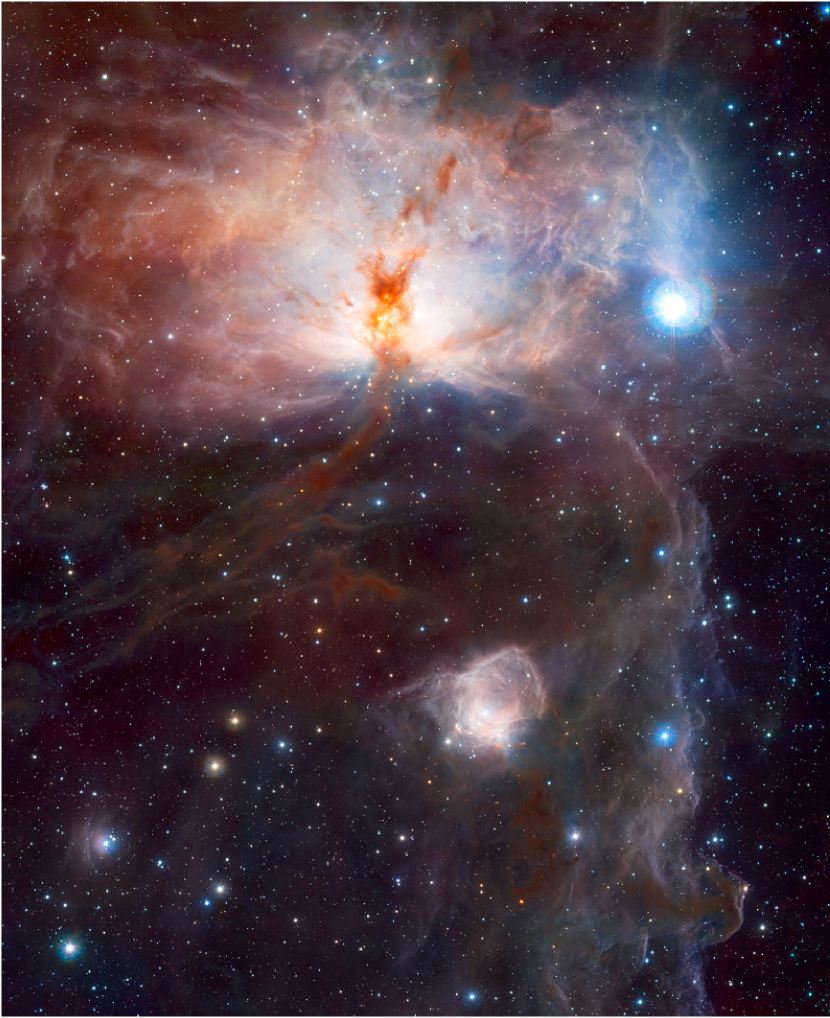
Figure 1: VISTA image of the Flame Nebula (NGC 2024). The obscuring dust lane that exists foreground to the bright Hii emission is seen almost transparent in this near infra-red image. The glow of NGC 2023 and the Horsehead Nebula are seen in the lower portion of the image.

NGC 2024 is the most active star forming region in the Orion B giant molecular cloud. The gas structure in this region has an ionized component surrounded by a background dense molecular ridge and a foreground dust and molecular component visible in the optical images as a dark lane. Recently, the new ESO telescope VISTA (Visible and Infrared Survey Telescope for Astronomy) released a high sensitivity near-infrared image of NGC 2024 (Figure 1). In this large scale view, the foreground dust lane which optically obscures the Hii region is almost transparent. Scattered light produced by the ionization front is seen as bright emission in the top of the image, and a cluster of hot young stars is revealed. Kandori et al. (2007) used near-infrared polarimetry to study the scattered light from the Hii region. Several reflection nebulae associated with young stellar objects (YSO) were discovered in their polarization maps. The overall centro-symmetric pattern suggests that the ionizing source is IRS 2b, a massive star located $5^{\prime\prime}$ north-west of IRS 2, in agreement with a previous near-infrared photometric study carried out by Bik et al. (2003). The submillimeter continuum emission arising from the dense molecular ridge was first observed by Mezger et al. (1988, 1992). Several far infrared cores (so the acronym “FIR”) at distinct evolutionary stages were identified and catalogued in a North-South (NS) distribution. In fact, the chain of FIR cores could have been generated by the interaction between the nearby Hii region and the surrounding molecular cloud. Fukuda & Hanawa (2000) performed numerical simulations of sequential star formation trigged by an expanding Hii region near a filamentary cloud. In their models, isothermal expansion and magnetohydrodynamic effects are considered. Their simulations preview that a chain of cores is formed from this interaction, each pair of cores belonging to a distinct generation though. Comparison between model and the dynamical parameters observed in NGC 2024 are quite good. In particular, they state that FIR 4 and FIR 5 belong to the first generation of cores, what is confirmed by the observed dynamical ages of their outflows. In this paper, we center our discussion on FIR 5, the brightest and most evolved of them, with a strong and collimated unipolar outflow (Richer et al., 1992). Continuum observations at 3 mm performed by Wiesemeyer et al. (1997) suggest that FIR 5 is a double core embedded in an envelope. However, higher angular resolution observations from Lai et al. (2002) (LCGR02 from now on) resolved the dust emission in one strong component surrounded by several weaker components in a radius of a few arcseconds.

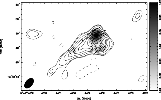
Figure 4: Contour map of the dust continuum emission overlapped with the linear polarization vectors (black vectors) towards NGC 2024 FIR 5. Gray scale correspond to the polarized dust intensity. Contours levels are $-3$, 3, 4, 7, 11, 16, 22, 32, 42, 52, 62–$\times$ the rms noise of the dust emission ($\sim 19$ mJy beam^-1). The length of each segment is proportional to the degree of polarization (the length corresponding to a polarization level of 10% is indicated at the image bottom) . The synthesized beam is of $2\farcs 45\times 1\farcs 48$ with a position angle of $-40\arcdeg$. Vectors are sampled as 2/3 of a beam.

Several authors have conducted polarimetric investigations toward FIR 5. Crutcher et al. (1999) used the Very Large Array (VLA) to carry out Zeeman observations of OH and Hi absorption lines in order to trace the line-of-sight (LOS) component of the magnetic field. These authors found a LOS field gradient of $\sim 100~{}\mu$G across the northeast-southwest direction. Dust emission polarization in the surroundings of FIR 5 was mapped in 100 $\mu$m by Hildebrand et al. (1995) and Dotson et al. (2000) with the Kuiper Airborne Observatory. At longer wavelengths, Matthews et al. (2002) used the SCUBA polarimeter to observe the 850 $\mu$m emission with at the James Clerk Maxwell Telescope (JCMT) and obtained polarization patterns consistent with those derived with the 100 $\mu$m data. Their single-dish dust polarization maps trace a relatively ordered magnetic field along the ridge of emission containing FIR 4 and FIR 5 (Fig. 4 in their paper). Based on the spatial coverage of their observations, this ordered field must extend over a distance of at least $\sim 0.5$ pc (for the assumed distance of 415 pc to the Orion B cloud). Matthews et al. (2002) modeled this field using a helical-field geometry threading a curved filament, since this configuration suited fairly to a 2-dimensional projection accordingly to the SCUBA maps. However, they found that this geometry is not consistent with the LOS Zeeman data of Crutcher et al. (1999) because no reversed fields are seen at both sides of the chain of cores. Instead, those authors offer another interpretation based on a compression zone created due to the expansion of the foreground ionization front. In this scenario, the magnetic field lines are stretched around the ridge of dense cores in a physical morphology consistent with LOS field gradient observed in the Zeeman data of Crutcher et al. (1999).

Concerning the local field associated with FIR 5, the work of Lai et al. (2002, hereafter LCGR02) has the best resolution for the dust continuum emission so far. These authors used the Berkeley-Illinois-Maryland-Association (BIMA array) interferometer and obtained an angular resolution of $2\farcs 4\times 1\farcs 4$. The polarized flux of the BIMA maps extends in a N-S direction, perpendicular to the putative protostellar disk. The corresponding field lines were fitted with a geometric model consisting of a set of concentric parabolas, indicating that the polarized flux trace a partial hourglass morphology for the magnetic field. In this paper, we report SMA dust continuum polarization toward FIR 5. The higher sensitivity of this instrument provides new information on the detailed field morphology of the FIR 5 core.

2 Observations and Data Reduction

The high angular resolution of the SMA allows us to trace the thermal emission of dust grains at physical scales of few hundred astronomical units (for objects in the Orion molecular cloud complex) and, therefore, is able to spatially resolve compact dust cores. A detailed description of SMA is given in Ho et al. (2004). The observations were carried out in 2007 November 24 and December 19 with the SMA in its compact configuration. The number of antennas available for the observations were 7 and 6, respectively. The atmospheric opacity at 225 GHz was 0.11 and 0.07 for the first and second day, respectively (values measured by the Caltech Submillimeter Observatory tau meter). Observations were done in the 345 GHz atmospheric window, what corresponds to a wavelength of 870 $\mu$m. The SMA receivers operate in two sidebands separated by $\sim 10$ GHz. The central observed frequencies for the lower and upper side bands were 336.5 GHz and 346.5 GHz, respectively. The SMA correlator had a bandwidth of 1.9 GHz (for each sideband) divided in 24 “chunks” of 128 channels each. In total, the full-band spectrum contains 3072 channels for each sideband and a spectral resolution of 0.62 MHz, which corresponds to a velocity resolution of 0.7 km s^-1. SMA receivers are single linearly polarized. By using a quarter-wave plate in front of each receiver, the incoming radiation is converted into circular polarization (L, R). The SMA correlator combines the signal into circular polarization vectors: RR, LL, RL, LR. In order to obtain the full four Stokes parameters for all the baselines, the visibilities have to be averaged on a time scale of 5 minutes. A description of the SMA polarimeter and the discussion of the methodology (both hardware and software aspects) are available in Marrone et al. (2006) and Marrone & Rao (2008).

The phase center ($\alpha_{2000}=05^{\mathrm{h}}41^{\mathrm{m}}44\fs 3$, $\delta_{2000}=-01\arcdeg 55^{\prime}40\farcs 8$) was set according to the peak of emission obtained for FIR 5 in LCGR02. Uranus and Titan were observed as flux calibrators in both tracks. The resulting visibility function for each calibrator is consistent with the expected flux estimated by the SMA Planetary Visibility Function Calculator during the observing runs. The quasar J0528+134 was used as the gain calibrator. The quasar 3c454.3 was used for bandpass and polarization calibration. The first track had a much better parallactic angle coverage for 3c454.3 than the second track, thus the 3c454.3 data from the first track were used to solve for the instrumental polarization or “leakages”. The minimum and maximum UV distance for both tracks was 16 and 88 k$\lambda$, respectively. Antenna 3 was used only in the second track, so no leakage solution could be derived. Thus, antenna 3 was not used to obtain Stokes Q and U maps. After the calibration steps, data from upper and lower sidebands for each track were synthesized into a single data set. Calibrated visibilities for each track were combined into a final data set. Removal of continuum contamination from the line data set was done. The main contribution arose from the CO ($3\rightarrow 2$) transition at the chunk # 4 of the upper sideband ($\sim 345.76$ GHz).

All the calibration and reduction steps were done with MIRIAD configured for SMA data (Wright & Sault, 1993). The science target was strong enough and self-calibration was performed in order to increase the signal-to-noise ratio in the final maps. Imaging of the Stokes parameters I, Q and U was performed. Maps of polarized intensity ($I_{P}$), polarized fraction ($P$) and position of polarization angles ($\theta$) were obtained by combining Q and U images in such a way that $P=\frac{I_{P}}{\mathrm{I}}=\frac{\sqrt{Q^{2}+U^{2}}}{\mathrm{I}}$ and $\theta=\frac{1}{2}\mathrm{tan}^{-1}(\frac{U}{Q})$. The resulting synthesized beam of Stokes I maps has $2\farcs 45\times 1\farcs 48$, with a position angle (PA) of $-39.8\arcdeg$. Table 1 summarizes the technical parameters of continuum and line observations.

3 Results

3.1 Dust Continuum Emission

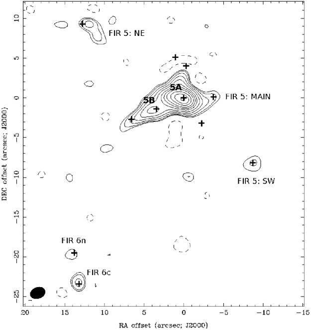
Figure 2: Dust continuum map of FIR 5 with quasi-uniform weighting ($robust=-1$). Contours are drawn at $-3$, 3, 4, 6, 9, 13, 19, 25, 32, 42, 52, 62 $\sigma$ (1–$\sigma\simeq 18$ mJy beam^-1). The half power beam width (HPBW) of the synthesized beam is $1\farcs 96\times 1\farcs 41$ and the position angle is $-70.6\arcdeg$. The crosses indicate the dust continuum sources detected by Lai et al. (2002) with BIMA.

Figure 2 shows the contour map of the 878 $\mu$m dust emission in FIR 5 obtained with a quasi-uniform weighting (a robust of $-1$), which provides a better angular resolution of $1\farcs 96\times 1\farcs 41$. The overall submillimeter emission resembles the 1.3 mm dust continuum maps obtained with BIMA by LCGR02, although the latter has a $rms$ a factor of 3 lower. Our observations (with shortest baseline equal to 16 k$\lambda$) allow us to only measure structures smaller than $\sim$ 5.7 arcseconds (see Equation A.5 of Palau et al. (2010)). In LCGR02, they find extended emission at scales of 5-7 arcseconds with BIMA. The brightest emission arises around FIR 5: Main (following LCGR02 notation), which is resolved into two components, 5A and 5B. Those components correspond to the double source detected in 3 mm by Wiesemeyer et al. (1997) and indentified as FIR 5-w and FIR 5-e. However, not all the fainter sources observed in the FIR 5: Main core of LCGR02 have been detected with the SMA. FIR 5: Main appears more extended in the BIMA maps, attributable to the better sampling of shorter baselines with the BIMA array. In particular, the N-S direction contains emission of the dust condensations LCGR2, LCGR3 and LCGR5 (according to LCGR02 nomenclature). These sources are missing in our SMA maps probably due to the absence of antenna 3 in the deconvolved maps (see section 2). Antennas 3 and 6 cover a short baseline in the UV plane which is parallel to the U axis and close to $V=0$ k$\lambda$. In equatorial coordinates, it corresponds to features parallel to the declination axis, and close to the phase center. Therefore, by flagging antenna 3 we lost this flux component which should be produced by the missing sources. In addition, different visibility sampling between the two aperture synthesis telescopes (BIMA sampled shorter baselines) must also be considered. We also detect several faint peaks (at the 4 and 7–$\sigma$ level; 1 $\sigma=18$ mJy beam^-1) also seen by LCGR02.

Tables  2 and 3 give the dust emission properties for the two condensations associated with FIR 5: Main and for the fainter dust condensations, respectively. The intensity peak and the position of the sources were derived using the Miriad task “maxfit”. For the two bright sources associated with FIR 5: Main, a two Gaussian fit (using the AIPS’s “imfit” task) was used to estimate the flux density of each component and its size. The two sources appear resolved but in different directions. Thus, source 5A has a full width half maximum (FWHM) size of $2\farcs 8\times 2\farcs 4$ elongated close to the NE–SW axis ($PA=67\arcdeg$), whereas source 5B has a deconvolved FWHM size of $3\farcs 6\times 2\farcs 8$ but is elongated along the SE–NW direction ($PA=124\arcdeg$).

In order to estimate the column density and mass of the cores, we need to assume a value for the cores’ temperatures. Different molecular line observations have established that the NGC 2024 cores are warm with temperatures between 40 and 85 K (Ho et al., 1993; Mangum et al., 1999; Watanabe & Mitchell, 2008; Emprechtinger et al., 2009). Here we adopt a temperature of 60 K. We assume a dust opacity at 878 $\mu$m of 1.5 cm² g^-1, which approximately is the expected value for dust grains with thin dust mantles at densities of $\sim 10^{6}$ cm^-3 (Ossenkopf & Henning, 1994). Using the previous FWHM sizes derived from the Gaussian fit, a beam-averaged column density of $\sim 4.7\times 10^{23}$ and $2.2\times 10^{23}$ cm^-2 for sources 5A and 5B were derived, respectively. Similarly, masses for these two components are 1.09 and 0.38 M_⊙, respectively. The total mass of FIR 5:Main, 1.5 M_⊙, is consistent with the value derived by Chandler & Carlstrom (1996).

3.2 Distribution of the polarized flux

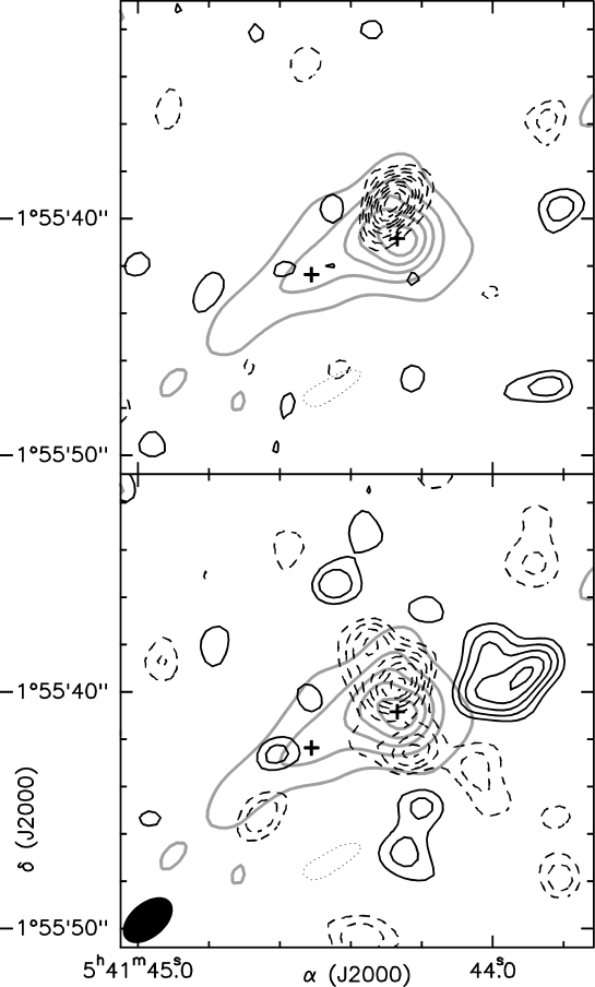
Figure 3: Maps of Stokes $Q$ (top panel) and $U$ (bottom panel) emission. Dashed and solid thin contours correspond to negative and positive polarized emission, repectively. The contours start at $-2$–$\sigma$ and 2–$\sigma$ level with steps of 1–$\sigma$ (1–$\sigma=5.3$ mJy beam^-1). The absolute $Q$ and $U$ peak fluxes are 0.056 Jy beam^-1and 0.047 Jy beam^-1, respectively. The thick grey contours show the Stokes I emission. Crosses indicate the position of the two dust intensity peaks. The synthesized beam of the maps is shown in the bottom left corner of the bottom panel.

For better sensitivity to the weak polarized emission, maps of Stokes I, Q and U were obtained with a robust weight of 0.50. Figure 3 shows the Stokes Q and U emission, which have different distributions. The Stokes Q emission arises from a negative compact spot about one arcsecond north of source A. The Stokes U is quite extended along FIR5: Main, with the brightest emission around source 5A. Source 5B has only weak polarized emission at 3–$\sigma$ level. It is noteworthy that significant positive Stokes U emission appears west of source 5A without dust emission associated. However, this spot of polarized emission coincides with the BIMA continuum source FIR 5: LCGR 1 (catalogue of LCGR02). The non-detection by the SMA could occur because dust emission has been resolved out by the interferometer (approximately 30% of the flux is filtered out, see section 3.1). Thus, we tentatively associated this polarized spot to this source. A cutoff of 2–$\sigma$ (1– $\sigma\simeq 5$ mJy beam^-1) in polarized intensity ($\sqrt{Q^{2}+U^{2}}$) is used to obtain the linear polarization emission and to derive the position angle in the plane of the sky of the polarization vectors.

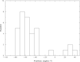
Figure 5: Histogram of position of polarization angles. The three polarized components of FIR 5 polarization map are clearly seen in this plot.

The polarization intensity and the polarization fraction in our maps achieve values as high as 54 $\pm$ 6 mJy beam^-1 and 15% $\pm$ 2%, respectively, at the northern portions of the core, where the polarized emission is brighter. Figure 4 shows the dust continuum emission from the protostar overlaid with the dust polarization vectors. Using the position of the continuum peak as reference, three main components can be distinguished: a northern component, where the highest polarization degrees are obtained, a southwestern component and an eastern component offset by $\approx 5^{\prime\prime}$ from the continuum peak. This distribution is well represented in the histogram of polarization angles shown in Figure 5. There is a change of roughly 90$\arcdeg$ in the position angles of vectors associated with FIR 5A and the eastern vectors associated with FIR 5B. Concerning only vectors associated with FIR 5A, position angles have a gradual rotation of approximately 40$\arcdeg$ from north to south. Table 4 summarizes our polarization data. Note that the distribution of the polarized flux of the SMA data is remarkably consistent with the BIMA maps of LCGR02. Although the structure of emission in both the BIMA and SMA data sets has the same overall pattern, the latter has a larger area of polarized flux. Compared to the JCMT maps of Matthews et al. (2002), the mean direction of our SMA polarization field is consistent with the lower resolution single-dish data, which do not resolve the structure of FIR 5 and traces a larger physical scale associated with the diffuse gas found at the core envelope.

3.3 CO (3 $\rightarrow$ 2) emission

Our SMA CO (3 $\rightarrow$ 2) maps reveal a very complex morphology possibly related to multiple outflows. Figure 6 shows the channel maps of the CO (3 $\rightarrow$ 2) emission with a velocity resolution of $\sim 2.1$ km s^-1. At blueshifted velocities the emission arises from an elongated but wiggling structure in the East-West direction. This blueshifted component appears to be associated with FIR 6. The distribution of the molecular gas at the cloud systemic velocity ($v_{\rm LSR}$ $\simeq 10$ km s^-1) is basically associated with the FIR 5 main core. At redshifted velocities ($v_{\rm LSR}$ $\gtrsim 14$ km s^-1) there are two main elongated features almost parallel extending in the North–South direction and observed over a wide range of velocities (up to $v_{\rm LSR}$ $\simeq 30$ km s^-1). One of these features is associated with the well-know outflow powered by FIR 5A (Sanders & Willner, 1985; Richer et al., 1992; Chandler & Carlstrom, 1996) and the other one is located about $10^{\prime\prime}$ to the west and seems to arise from FIR 5-sw. These two lobes have their brightest emission located near their associated dust components (FIR 5A and sw). The emission presents a clumpy morphology, with an average angular size of $\sim 5^{\prime\prime}$, corresponding to a physical size of 0.01 parsecs. It is worth noting that the three possible CO high velocity features have no counterpart at the opposite flow velocities. Thus, the North-South redshifted lobes have no blueshifted counterpart, and the East–West blueshifted lobe does not have a redshifted counterpart.

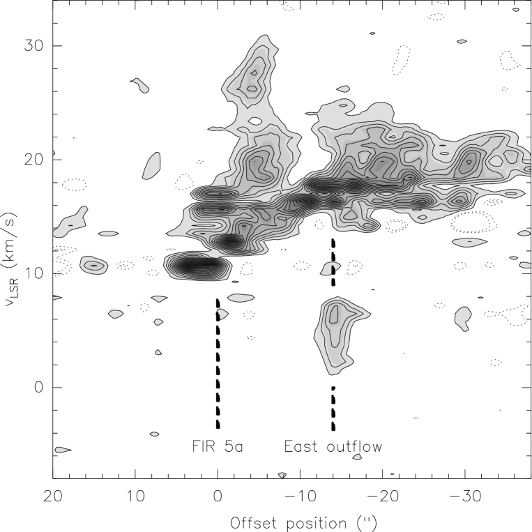
Figure 7: Position-Velocity plot of the CO ($3\rightarrow 2$) emission centered close to source FIR 5A (one arcsecond to the west) and along the North (positive offsets) to South (negative offsets) direction. Contours levels are $-5$, $-3$, 3, and then steps of 3 times 0.3 Jy beam^-1, the $rms$ noise of the channel maps where the cut was obtained. The position of the driving source of the redshifted outflow, FIR 5A, is indicated with a dashed line. The spatial overlap with the East ouftflow associated with FIR 6 is also shown with a dashed line.

Figure 7 shows the Position-Velocity (PV) diagram centered in FIR 5A with a PA = 0$\arcdeg\!$.9 (along the brightest redshifted lobe). The outflow powered by FIR 5A has a wide distribution of velocities which prevails until $\sim 30$ km s^-1. An extended spatial distribution is observed up to $\sim 35^{\prime\prime}$ south of the source, although only low velocity components are observed at such distances. No blue lobe is seen and only residual emission is measured in the northern counterpart. The blue component observed at the offset position of $-14^{\prime\prime}$ is part of the outflow associated with FIR 6. In section 4.4 we provide a detailed discussion about the molecular distribution in this region.

4 Discussion

4.1 Polarization properties

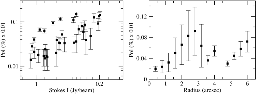
Figure 8: Distribution of polarization toward NGC 2024 FIR 5. Left panel: Polarization intensity versus total intensity. Right panel: Polarization intensity versus radius with respect to the peak of Stokes I emission.

In this section, we focus our analysis on the northern and southwestern polarization features, which are the brightest components and scientifically more interesting since a less uniform pattern is observed. At 2-$\sigma$ level, these two regions are connected and surround the peak of total intensity. From Figure 4, it can be noted that the peak of polarized and total intensities are approximately $2\farcs 6$ apart. Figure 8 shows the dependence of the polarization fraction with Stokes I flux and with respect to the distance to source A. In both cases, there is a clear depolarization toward the center, where the highest density portions of the core are located. The left panel of Figure 8 suggests that the distribution of polarization with respect to the Stokes I emission seems to be composed by two subsets: the highest polarization fraction data that has a slower growing curve and corresponds to the northern component, and the subset with a linear dependence, which arises from the southwestern component. The right panel of Figure 8 was produced by performing averaging over polarization data for concentric annuli of $0\farcs 4$ each.

The depolarization effect is observed not only at the brightest component, source A, but also for the second dust component, source B, represented by a “hole” at $r\simeq 4\farcs 5$ in the right panel of Figure 8. Those diagrams are consistent with Figure 4, where the polarization fraction increases with distance from the peak of emission, but there is a lack of overall polarized emission toward source B.

The depolarization observed at higher values of Stokes I seems to be part of a global effect observed at different wavelengths (Goodman et al., 1995; Lazarian et al., 1997). In the mm/submm range, this phenomenon was also observed in the BIMA data published by LCGR02, as well as far-infrared observations with single dishes (Schleuning, 1998; Matthews et al., 2001) . The anti-correlation between Stokes I and polarization fraction can be caused by different mechanisms. On one hand, it may be the result of changes in the grain structure at higher densities. Those changes may be responsible for a decrease in the efficiency of dust grain alignment with respect to the local magnetic field (Lazarian & Hoang, 2007). In the case of FIR 5B, the embedded source may be in a very early stage of formation, prior even to collapse (since no clear evidence of star-forming signatures like outflows has been assigned to it). In this case, the lack of internal infrared radiation could provide no radiative torque to the dust grains and, therefore, no polarized flux is observed. Another explanation for this effect could be a twisted magnetic field or the superposition of distinct field directions along the LOS resulting in a reduction of the net polarization degree (Matthews et al., 2001). Observations at higher angular resolution would be necessary to resolve the small scale structure.

4.2 Magnetic field properties

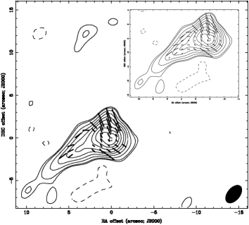
Figure 9: Plane-of-sky field geometry for NGC 2024 FIR 5. Contours, beam and vector scale are the same than in Figure 4. Vectors are plotted at 2$\sigma_{\mathrm{P}}$ level and relaxed to 1$\sigma_{\mathrm{P}}$ in the upper right corner.

In section 1 we briefly introduce the physical mechanisms associated with the alignment of dust grains with respect to the magnetic field lines. Although some works propose that grain alignment could be independent of magnetic fields (e. g.: mechanical alignment by particle flux, Gold (1952)), it has not been proven yet observationally. Dust grains are believed to have at least a small fraction of atoms containing magnetic momentum in their compositions, so some interaction with the ambient magnetic field is expected. The most stable energy state is achieved when the grain longest axis rotates perpendicularly to the field lines. Consequently, dust emission polarization vectors as observed in submillimeter polarimetry have to be rotated by 90$\arcdeg$ in order to be parallel to the plane-of-sky (POS) component of the magnetic field. The LOS field component adds no information to the 2D polarization map because the spinning dust grains produce zero polarization flux. If a strong LOS component is expected, a decrease in net polarization flux is observed, and alternative techniques must be used to measure it (e.g., Zeeman effect observations: Troland & Heiles (1982); Crutcher et al. (1993)). Therefore, the polarization map of Figure 4, when rotated by 90$\arcdeg$, traces the projection of the 3D magnetic field morphology on the plane-of-sky (see Figure 9). For FIR 5A, the field geometry is described by curved lines centered on the protostellar core. Toward the elongated emission associated with FIR 5B, the field lines are parallel to the core’s major axis, implying a 90$\arcdeg$ change in the direction with respect to the FIR 5A mean direction. By relaxing the signal-to-noise level down to 1–$\sigma$, one can see that this change in the magnetic field direction is not abrupt, and an hourglass morphology can be roughly derived for the main component (Figure 9, upper right box). Several theoretical works have performed 3D simulations of collapsing magnetized clouds. They all agree that the POS projection of the magnetic field morphology in those class of objects is a hourglass shape (Ostriker et al., 2001; Gonçalves et al., 2008). Our results, and many others (e.g. Girart et al. (2006); Rao et al. (2009)) provide observational support to these models.

So far, the CF relation developed by Chandrasekhar & Fermi (1953) is still the most straightforward method to estimate the plane-of-sky component of the magnetic field. Assuming energy equipartition between kinetic and perturbed magnetic energies as

$$\frac{1}{2}\rho\delta V^{2}_{LOS}\simeq\frac{1}{8\pi}\delta B^{2},$$ (1)

(where $\delta V_{LOS}$ is the observational rms velocity along the line-of-sight and $\rho$ is the average density), this method compares the fraction of uniform to random components of the field under effects of Alfvénic perturbations ($\delta v\propto\delta B\sqrt{\rho}$) taking into account isotropic velocity dispersions. The CF formula uses the dispersion of position of polarization angles and molecular line widths as observational inputs for the gas motions in the core. However, recent works showed that this approximation overestimates the magnetic field for coarser resolutions (Heitsch et al., 2001; Ostriker et al., 2001). These authors constrained the application of this method to data sets with relatively low dispersion of position angles ($\Delta\theta\leq 25\arcdeg$), which means strong-field cases. By statistical studies of magnetic turbulent clouds, these authors showed that the CF formula is accurate only if this condition is applied. Using the small angle approximation $\delta\phi\approx\delta B/B_{uniform}$, the CF formula can be stated as follows:

$$B_{uniform}=\xi\sqrt{4\pi\rho}\frac{\delta V_{LOS}}{\delta\phi},$$ (2)

where $\delta\phi$ is the angle dispersion. The correction factor $\xi$ ($\simeq 0.5$) arises from the previously mentioned strong field conditions to which this case applies (Ostriker et al., 2001).

Unlike LCGR02, we opted for not applying any geometric model to the observed field due to the low statistics of our data set. The observed dispersion in our data (main component in the histogram of Figure 5) is 12.2$\arcdeg$. According to $\delta\phi_{obs}=(\delta\phi^{2}_{int}+\sigma_{\theta}^{2})^{1/2}$, the observed dispersion depends on the intrinsic dispersion $\delta\phi_{int}$ plus the measurement uncertainty of the position of the polarization angles $\sigma_{\theta}$, resulting from the contributions of both effects. Since that no geometric models were used to remove the systematic field structure, changes on the large-scale field directions are included in the intrinsic dispersion, together with turbulent fields due to Alfvénic motions. In our data set, the position angle uncertainties average to 7.52$\arcdeg$, which gives us an intrinsic dispersion of 9.61$\arcdeg$. Some extra observational parameters are needed to compute the magnetic field strength with equation 2. The average density and the rms velocity in FIR 5 can be obtained from previous works. Emprechtinger et al. (2009) modeled the morphology of NGC 2024 based on APEX observations of CO isotopologues. The various line profiles obtained for different transitions are consistent with a complex structure composed by a Photo Dominated Region (PDR) foreground to the molecular gas where the far infrared cores are found. In their models, the dense molecular cloud must be warm (75 K) and dense ($9\times 10^{5}$ cm^-3) to reproduce the velocity gradients observed for distinct cloud components. These results agree with the previous work of Mangum et al. (1999), based on formaldehyde observations. These authors derived a kinetic temperature of $T_{K}>40$ K for FIR 3-7 and estimate densities at the same order of magnitude ($n_{\mathrm{H_{2}}}\approx 2\times 10^{6}$ cm^-3). We adopt $n_{\mathrm{H_{2}}}=1.5\times 10^{6}$ cm^-3 as an average value for the density. For the velocity dispersion, we adopt $\delta V_{LOS}$ of 0.87 $\pm$ 0.03 km s^-1, which is the value derived by Mangum et al. (1999) from the formaldehyde observations. This molecule is a good tracer of dense gas, and for the single-dish data of Mangum et al. (1999), it traces the gas kinetic temperature in a scale of $\sim 8000$ AU, hence it is well correlated to the turbulent motions of the core. Finally, applying those inputs to the equation 2, together with the $\delta\phi_{int}$ previously obtained, we estimate that the POS magnetic field strength is 2.2 mG, which is in good agreement with the value estimated in LCGR02. The uncertainty in the magnetic field strength is determined mainly by the error in the volume density $n$, which is a factor of $\sim$ 2 due to the distinct assumptions on the cloud temperature. This factor implies an uncertainty of 40% for the derived field strength. As mentioned earlier, the dispersion used as input in equation 2 carries the combined effects of changes on the large-scale field directions plus turbulent motions. In this case, the derived field strength is only a lower limit since the angle dispersion is not generated purely by Alfvénic motions. On the other hand, beam averaging and line-of-sight effects due to field twisting of multiple gas components usually underestimates the real value of the turbulent component, and the estimated field strength in this case would be an upper limit. So, we can assume that both effects cancel out and 2.2 mG is a fair estimation for the POS field strength.

The mass-to-flux ratio gives information on whether the magnetic field can support the cloud against the gravitational collapse and, therefore, it provides clues about the evolutionary state of the source. Specifically, this quantity compares the pressure produced by an amount of mass M in a magnetic tube of flux $\Phi$. A critical value, reached when the magnetic pressure is no longer able to support the gravitational pulling, is given by $(2\pi\sqrt{G})^{-1}$ (Nakano & Nakamura, 1978). Observationally, this parameter is defined by (Crutcher et al., 1999):

$$\lambda=\frac{(M/\Phi)_{observed}}{(M/\Phi)_{critical}}=(m{\mathrm{N(H_{2}})}A/BA)\times(2\pi\sqrt{G})=7.6\times 10^{-21}\frac{\mathrm{N(H_{2}})}{B},$$ (3)

where $(M/\Phi)_{critical}$ is the mass-to-flux ratio of an uniform disk where gravity is balanced by magnetic pressure, $m=2.8m_{H}$ allowing for He, $A$ is the cloud area covered by observations, N(H₂) is the column density and $B$ is the magnetic field strength. Applying the POS magnetic field strength obtained in the previous paragraph, $B=2.2$ mG, and the column densities derived in section 3.1, we estimate a mass-to-flux ratio for FIR 5A of 1.6 (for $T=60$ K), which corresponds to a core in a supercritical stage. In any case, those calculations are restricted to the dust envelope, without taking into account the mass contribution of the embedded protostar. We consider that the derived mass-to-flux values are only a lower limit for this quantity and therefore it is in agreement with the observed star-forming signatures.

We can also derive the ratio between turbulent and magnetic energies. From the autocorrelation function of the polarization position angles, it is possible to measure how the dispersion of PA’s varies with respect to the distinct length scales within the cloud. This function provides an indirect calculation of the turbulent to magnetic energy as (Hildebrand et al., 2009):

$$\beta_{turb}\approx 3.6\times 10^{-3}\left(\frac{\delta\phi}{1\arcdeg}\right)^{2}$$ (4)

For the angular dispersion obtained from our sample, $\delta\phi_{int}=9.61$, we compute the turbulent to magnetic energy ratio as $\beta_{turb}=0.33$. This value agrees with the ratio estimated in LCGR02, which reinforces that the turbulent motions are magnetically dominated. The turbulent-to-magnetic energy ratio found for FIR 5 is consistent with what was measured for other low-mass protostellar cores like NGC 1333 IRAS 4A and IRAS $16293-2422$ (Girart et al., 2006; Rao et al., 2009).

4.3 Magnetic field around FIR 5A: gravitational pulling or Hii compression?

In this section, we try to elucidate which mechanism is mainly responsible for the observed curved magnetic field morphology in FIR 5. One possibility is that the gravitational pulling overcomes the local magnetic support and drags the ionized material toward the center, warping the field lines in such a way that they assume an hourglass morphology. This is consistent with the previous result that the protostellar core is in the supercritical regime. However, if this is the case then only the hourglass component west of FIR 5A is observed. The lack of detected vectors east of FIR 5A could be due to the overlap in the line of sight of the dust polarization associated with both FIR 5A and FIR 5B cores. The magnetic field direction associated with FIR 5B is perpendicular to the FIR 5A main direction. Alternatively if the two cores are connected, then it could be due to an abrupt change in the magnetic field direction. In both cases, the net polarization flux is expected to decrease significantly. Another possibility is that the grain alignment efficiency associated with source B is smaller. Indeed, Figure 8b (right panel) show that the second polarization “hole” matches quite well to the position of FIR 5B. Of course, the cause could also be a combination of these possibilities.

If the tension generated by the magnetic field curvature is produced by the gravitational collapse, then we can make a rough estimation of the mass required to produce the observed curvature. This magnetic force can be expressed as $B^{2}/R$, where R is the radius of curvature of the field lines. According to the equations derived by Schleuning (1998), we have

$$\left[\frac{M}{100\mathrm{M_{\odot}}}\right]=\left[\frac{B}{1\mathrm{mG}}\right]^{2}\left[\frac{D}{0.1\mathrm{pc}}\right]^{2}\left[\frac{R}{0.5\mathrm{pc}}\right]^{-1}\left[\frac{n(\mathrm{H_{2}})}{10^{5}\mathrm{cm^{-3}}}\right]^{-1}$$ (5)

where $D$ is the distance of the field lines from the protostar. At $D=1\farcs 9$ (789 AU) the field lines have a radius of curvature R of $17^{\prime\prime}$ (7055 AU). At the selected radius of curvature, the estimation of magnetic tension force is $\sim 10^{-23}$ dyne cm^-3. Applying these values to equation 5, we find that the mass inside the radius of $1\farcs 9$ is $\simeq 2.3$ M_⊙. Although this value is almost a factor of two higher than the mass estimation done for FIR 5A in section 3.1, it is within the same order of magnitude of the first estimation, even with the large uncertainties in the assumptions of $D$ and the radius of curvature $R$. This method is an alternative approximation to test if gravitational pulling is the responsible for the magnetic field curvature.

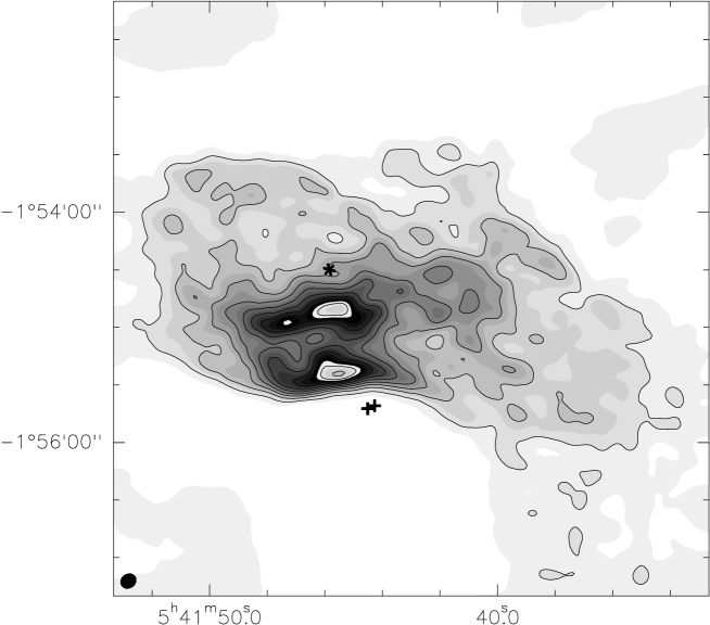
Figure 10: VLA 6 cm emission from the Hii region in NGC 2024 (data from the VLA Archive). Grey scale-filled contours are 0.5, 1.5, 2, 3, 4, 5, 6, 7, 9, 11, 13.1$\sigma$ (1$\sigma\simeq 9$ mJy beam^-1). The beam size of $8.6^{\prime\prime}\times 7.5^{\prime\prime}$ and PA of 37$\arcdeg$ is shown in the lower left corner. Crosses indicate the location of FIR 5A and FIR 5B sources. The star indicates the position of the ionization source.

Given the situation of the FIR 5 core, the external agents may also interfere in the protostellar physical environment. Previous observations proved that the molecular ridge and the chain cores in NGC 2024 are located at the far side of the Hii region (Barnes et al., 1989; Schulz et al., 1991; Chandler & Carlstrom, 1996; Crutcher et al., 1999). The distribution of molecular and ionized gas proposed by Matthews et al. (2002) for NGC 2024 (Figure 8 in their paper) has the western portion of the ionization front expanding toward the background molecular ridge and stretching the magnetic field lines around the ridge of dense cores. At large scales ($\sim 0.5$ pc), this morphology is corroborated not only by the LOS field obtained from the CN Zeeman observations (Crutcher et al., 1999) but also by the POS field from the single-dish dust polarization data. At smaller scales ($\sim 0.02$ pc), this could have an effect of compressing the magnetic field lines, bending them toward the east, as observed around the FIR 5 core. In order to check if the radiation pressure can be large enough to compress the molecular gas, we have studied the distribution of the ionized gas in NGC 2024. For this purpose, we accessed the NRAO Data Archive System to search for centimeter emission that could reproduce this morphology. We found an extended emission in 6 cm related to the Hii region produced by the star IRS 2b. Figure 10 shows that the hot gas has an extended component to the west and is roughly flattened to the south (although slightly curved to the southwest). FIR 5A and FIR 5B, indicated as crosses in Figure 10, lie in the border of the Hii region. The bright southern pattern near FIR 5 could trace the compressed ionized gas resulting from the interaction between hot/diffuse and cold/denser components. The radiation pressure produced by the illuminating star ($P_{\mathrm{rad}}$) can be calculated by $\frac{L}{cA}$, where $L$ is the luminosity of the ionization source, $c$ is the speed of light and $A$ is the area of the expanding shell. Bik et al. (2003) found that the spectral type of IRS 2b is in the range O8 V–B2 V, which is consistent with the intensities of radio continuum and recombination lines observed in the Hii region (Kruegel et al., 1982; Barnes et al., 1989). Therefore, we can assume $L=10^{5.2}L_{\odot}$, which is representative of such a spectral type. A first estimation for the radius of the Hii region was done by Schraml & Mezger (1969) through low resolution ($\sim 2^{\prime}$) radio observations of NGC 2024. These authors measured a radius of 0.2 pc ($\simeq 41\times 10^{3}$ AU) inferred from the observed emission. However, from Figure 10, the radius of the centimeter emission can be fairly estimated in $\sim 1^{\prime}$, which is approximately the distance between FIR 5 and IRS 2b. As a result, the radiation pressure $P_{\mathrm{rad}}$ is calculated as 1.16 $\times 10^{-8}$ dyne cm^-2. The ionization pressure ($N_{e}\times T_{e}\times k$) also accounts for the energy produced by the PDR. We assume an electron density of 5.94 $\times 10^{3}$ cm^-3 as derived from the emission parameters of the centimeter VLA map. The recombination line studies of Reifenstein et al. (1970) provide an electron temperature of 7200 K for this Hii region. To be conservative, we adopt a range of 7200–15000 K for $T_{e}$. With these parameters, the ionization pressure is estimated to range between $5.9\times 10^{-9}$ and $1.2\times 10^{-8}$ dyne cm^-2. On the other hand, the magnetic pressure is defined by $P_{mag}=\frac{B^{2}}{8\pi}$, where $B$ is the total magnetic field strength. Since our SMA maps provide a two-dimensional picture of the total field, we are able to calculate only a lower limit for the magnetic pressure. Therefore, applying the previous equation for the field strength obtained in section 4.2, we have $P_{mag}\geq 1.96\times 10^{-7}$ dyne cm^-2. This value is at least one order of magnitude higher than the radiation and ionization pressures. Even if we add the thermal pressure to the calculations ($P_{ther}\simeq 1.4\times 10^{-9}$ dyne cm^-2, Vallee (1987)), the energy injected by the ionization front is still lower than the magnetic force. Therefore the expanding Hii region is not enough to compress the magnetic field lines into the observed geometrical configuration, and the bending is produced by the gravitational pulling.

4.4 Multiple Outflows

Previous works reported that FIR 5 has an associated (redshifted) unipolar and highly collimated outflow with a mass of $\sim 4$ M_⊙ and density of $\sim 10^{2}$ cm^-3 (Sanders & Willner, 1985; Richer et al., 1992; Chandler & Carlstrom, 1996). However, a rather complex morphology was proposed by Chernin (1996) as indicated by their interferometric (BIMA) and single dish (NRAO 12 m telescope) combined maps of CO ($1\rightarrow 0$). In those, in addition to the unipolar lobe associated to FIR 5, there are two other redshifted features along the North-South direction and practically parallel to the FIR 5 molecular outflow, but neither of them associated with it. These two components were named $ns1$ and $ns2$ and are detected at $v_{\rm LSR}$ velocities between 15 and 25 km s^-1. $ns2$ is associated with FIR 6. They also identified a blueshifted feature, $ew1$, extending east of FIR 6. Chernin (1996) proposed that the brightest outflow component apparently powered by FIR 5A has a layered velocity structure. Their lower resolution combined molecular maps ($\sim 4\farcs 5$) are dominated by an unipolar red lobe composed by two parallel outflows at lower velocities ($\sim$ 20 km s^-1 in their Figure 1) which merge into only one at high velocities . This redder emission, referred as $ns1$ in their paper, is more collimated than the lower velocity components and arises $10^{\prime\prime}$ west of FIR 5: A. The author suggests that the $ns1$ outflow is widened by jet-wandering or internal shocks (Chernin & Masson, 1995) and is powered by a deeply embedded and undetected source rather than FIR 5A due to its misalignment with it.

In this work, we offer a different interpretation for this scenario. The SMA CO $(3\rightarrow 2)$ maps have an angular resolution a factor of 2 higher than the combined maps of Chernin (1996). Contrary to the suggestion by Chernin (1996), our maps show that this outflow is clearly powered by FIR 5A instead of by a faint, undetected low-mass star. The overall morphology described by Chernin (1996) is also observed in our maps. The main difference is that we detect high velocity gas which is offset by $10^{\prime\prime}$ west of FIR 5A, coinciding in position with the previously undetected FIR 5-sw dust condensation.Then, two interpretations can be derived from those features. Firstly, it is possible that all components are part of a single but velocity-layered outflow, the two low velocity lobes tracing the cavity where the highest velocity outflow is located. The presence of the high velocity lobe not only at the center of the cavity but also displaced from it could suggest that the outflow is precessing. Alternatively, the presence of the FIR 5-sw dust source associated with the western red shifted lobe, and in particular at high outflow velocities, suggest that this lobe could be an independent molecular outflow. As in the case of FIR 5A, this outflow would be also an unipolar outflow.

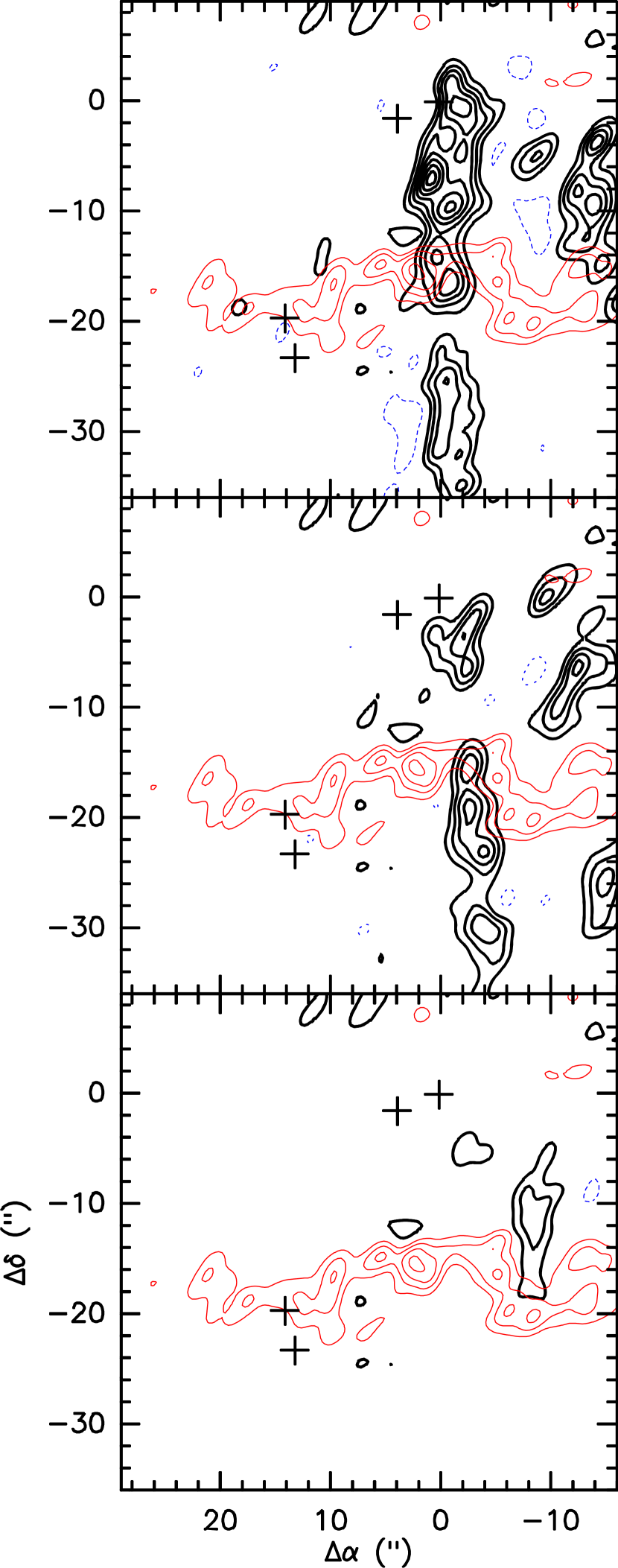
Figure 11: Superposition of contours from 15.6, 19.2 and 29.7 km s^-1velocity channels (black contours) over 7.2 km s^-1channel (red contours). Intensity contours are -3, 3, 4, 5, 7, 9, 12 $\sigma$ (1 $\sigma\approx 0.57$ mJy beam^-1). Source positions are maked as crosses.

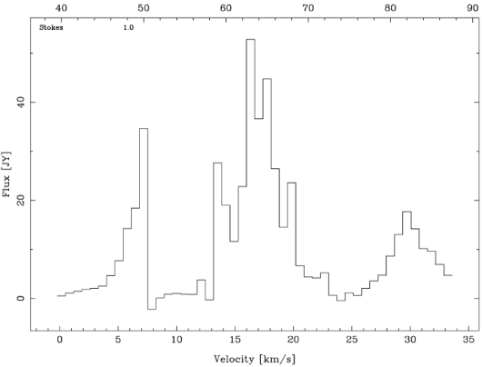
Figure 12: Spectrum of the interacting zone between the EW outflow, powered by FIR 6, and the high velocity feature apparently powered by FIR 5-sw. The spectrum was obtained for a velocity range of 0 to 33.2 km s^-1. The three peaks correspond to the emission from the EW outflow (the blue shifted peak at $\sim$ 7 km s^-1), the main lobe powered by FIR 5A at $\sim$ 18 km s^-1and the high velocity lobe arising from FIR 5-sw at $\sim$ 30 km s^-1.

Our CO $(3\rightarrow 2)$ maps seem to indicate a possible interaction between the different outflows. In the blue lobe of Figure 6, there is extended emission centered in the dust condensation FIR 6n (using the LCGR02 nomenclature) with an EW orientation. The emission is associated with an unipolar outflow detected from $\sim$ 1.0 to 7.8 km s^-1 and is characterized by a wandering/wiggling morphology. The outflow suffers structural changes in its shape, represented by drastic rotations in PA. From being powered initially toward the NW direction, it assumes an almost horizontal distribution (PA = 94°) which corresponds to its brightest emission. Then, another structural change seen at 7.8 km s^-1 results in an $u-$like shape. Both the bending from NW to the EW direction and the $u-$like structure coincide spatially with the projection of the red-lobe NS outflows powered by FIR 5A and FIR 5: sw. Figure 11 shows contours of velocity channels 15.6, 19.2 and 29.7 km s^-1 (black contours) overlaid with the 7.2 km s^-1 channel (red contours) in the upper, middle and bottom panels, respectively. The variations in PA of the EW outflow may be somehow due to the interaction with the main outflow powered by FIR 5A and the high velocity emission from FIR 5-sw. Global inspection of these three panels tentatively leads to the hypothesis of a shock interaction between distinct outflows in such a way that the gas structure is modified. The spectrum exhibited in Figure 12 was obtained for the supposedly interacting zone of the panels of Figure 11. A box of $-6^{\prime\prime}<\Delta\alpha<-18^{\prime\prime}$ and $-9^{\prime\prime}<\Delta\delta<-24^{\prime\prime}$ was used to select a region where all three outflows components (EW, main and high velocity features) contribute to the emission. The lack of CO emission seen at $\sim$ 25 km s^-1 is probably due to the cavity previously mentioned and corresponds to the velocity interval between low and high red velocity components. The blue emission is related to the EW outflow.

4.5 Unipolar molecular outflow

Previous observations of NGC 2024 fail to detect a blue counterpart for the bright outflow powered by FIR 5A (Richer et al., 1992; Chernin, 1996). However, other studies claim a bipolarity for this outflow (Sanders & Willner, 1985; Barnes et al., 1989). In all cases, the red shift lobe which is ejected toward the south has a brighter, more extended and collimated emission than the putative blue counterpart. These works all identify this feature as the main component of this outflow, making the morphology of the blue lobe, if it really exists, of unclear nature.

This asymmetrical pattern of the outflow powered by FIR 5A could be explained by the cloud morphology proposed by Matthews et al. (2002), illustrated in Figures 6 and 8 in their paper. They indicate how the NGC 2024 Hii region could be seen from the west and north directions, respectively. In this scenario, the dust cores appear in the dense molecular cloud behind the Hii expanding front (using the line-of-sight as reference), with FIR 5 projected right below the interface zone. Consequently, the bipolar molecular outflow ejected from this core will have the blue molecular component destroyed by the UV photons produced in the Hii region, since it points right toward it, but the red lobe would remain intact. Despite the fact that Barnes et al. (1989) did not know accurately which core is the driving source of the supposedly blue outflow, these authors found that the total luminosity of the nebula is comparable to the flow energy. Therefore, some interaction between both could be expected.

5 Conclusions

In this paper, we report SMA polarization observations of the intermediate-mass protostellar core NGC 2024 FIR 5. Data acquisition was done using the polarimetric capabilities of the SMA combined with wide spectral window receivers. The polarized flux appears distributed in three components: two of them around the peak of total intensity (Stokes I) and another component arising from the elongated portion of the core. The overall polarization portion resembles a partial hourglass morphology due to a possible ambipolar diffusion phenomenon taking place in the core.

The magnetic field strength was estimated in 2.2 mG. The estimates of turbulent-to-magnetic energy and mass-to-flux ratio are consistent with a supercritical highly magnetized core. In previous works, magnetized collapsing cores were also observed in high-mass protostars. In general, ambipolar diffusion seems to affect core evolution globally, independent of the mass range.

The absence of a symmetrical field morphology gives rise to different interpretations for the field structure in the core. The dust cores in NGC 2024 may be affected by an expanding ionization front compressing the molecular gas. It could be perturbing the field structure at smaller scales. The bended lines observed in our SMA maps could be the consequence of the radiation pressure of the hot component. Previous VLA 6 cm observations trace the foreground Hii region as an extended emission produced by the O2–B2 ionization source IRS 2b. However, our estimations of radiation pressure due to the expanding shell does not overcome the magnetic pressure generated by the field lines. So, the asymmetrical magnetic field is more likely due to depolarization effects arising in the position of the previously unresolved FIR 5B source.

A complex outflow morphology was observed toward FIR 5. Several collimated features were detected toward FIR 5, FIR 6 and FIR 5-sw. We speculate about a possible flow interaction between distinct components. It could explain the structural changes observed in some outflows. The brighter emission powered by FIR 5A has a clumpy structure and arises highly collimated in a NS orientation. The absence of a blue lobe counterpart can be attributed to the expanding Hii region to the north of the core. The UV radiation field may be responsible for dissociating the molecular structure of the outflow, destroying this component.

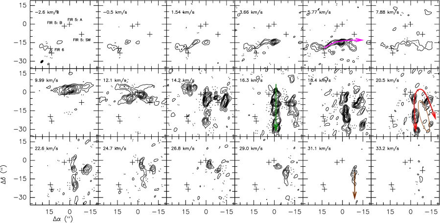
Figure 6: Channel maps of the CO ($3\rightarrow 2$) emission associated to FIR 5 and FIR 6 dust cores. Contours levels are -4, 4, 8, 12, …to 36 $\times$ 0.25 mJy beam^-1(the rms noise of the map). The value of the V_LSR is shown in the top left corner of each panel. Source positions are indicated as crosses and labelled in the first panel. Magenta, green, red and brown arrows indicate the position of the FIR 6, FIR 5A, the precessing and the FIR 5-sw outflows respectively. An ellipse indicates the supposedly cavity produced by the high-velocity components of the main FIR 5 outflow component.

Table 1: Parameters of the continuum and line observations

Observations	Rest frequency	HPBW	PA	Spectral resolution	Peak of emission	$rms$ noise
	(GHz)	(arcsec)	($\arcdeg$)	km s-1	(Jy beam-1)	(Jy beam-1)
Continuum	345.8000	$2.45\times 1.48$	-39.8	–	1.19	0.019
CO (3$\rightarrow$2)	345.7960	2.87 $\times$ 1.67	-37.6	0.7	9.5	0.57

Table 2: FIR 5: main component

Dust	$\alpha_{2000}$	$\delta_{2000}$	Peak	Total	FWHM	Deconvolved	Deconvolved
condensation			of intensity	flux	Gaussian fit	size	PA
			(Jy beam-1)	(Jy)	(arcsec)	(arcsec)	($\arcdeg$)
FIR 5A	05 41 44.258	$-01$ 55 40.94	1.16(2)	2.44(6)	2.8 $\times$ 2.4	2.31(6)$\times$1.58(8)	47(5)
FIR 5B	05 41 44.510	$-01$ 55 42.35	0.40(2)	1.26(8)	3.6 $\times$ 2.8	3.1(2)$\times$2.3(1)	130(11)

Note. — Units of right ascension are hours, minutes and seconds, and units of declination are degrees, arcminutes, and arcseconds.

Table 3: Sub-millimeter dust condensations

Dust	$\alpha_{2000}$	$\delta_{2000}$	Peak	Flux
condensation			of intensity	density
			(mJy beam-1)	(mJy)
FIR 5-sw	05 41 43.667	-01 55 49.05	77(18)	81(21)
FIR 5-ne	05 41 45.043	-01 55 31.60	131(18)	202(30)
FIR 6n	05 41 45.193	-01 56 00.50	70(18)	40(15)
FIR 6c	05 41 45.134	-01 56 04.01	124(18)	116(22)

Table 4: SMA polarization data from NGC 2024 FIR 5

$\Delta$ RA	$\Delta$ Dec	P	$\epsilon$P	$\sigma_{P}$	IP	$\theta$	$\epsilon\theta$
(arcsec)	(arcsec)	(%)	(%)		(Jy beam-1)	($\arcdeg$)	($\arcdeg$)
5.4	-2.1	6.00	2.0	3.00	0.018	35.723	9.194
0	-2.1	13.4	3.1	4.32	0.027	-34.364	6.093
5.4	-1.5	9.20	2.8	3.29	0.019	27.954	8.355
4.5	-1.5	3.40	1.4	2.43	0.013	24.122	12.244
1.8	-1.5	3.60	1.6	2.25	0.013	-48.573	12.838
0.9	-1.5	3.30	1.2	2.75	0.016	-47.342	10.207
0	-1.5	5.20	1.1	4.73	0.027	-35.171	6.1
-0.9	-1.5	8.00	1.9	4.21	0.025	-34.346	6.549
1.8	-0.9	2.00	1.0	2.00	0.012	-49.173	13.955
0.9	-0.9	1.70	0.7	2.43	0.014	-55.723	11.734
0	-0.9	1.80	0.6	3.00	0.017	-39.46	9.757
-0.9	-0.9	3.40	1.0	3.40	0.019	-37.513	8.696
1.8	-0.3	1.50	0.7	2.14	0.012	-60.593	13.363
0.9	-0.3	2.10	0.6	3.50	0.022	-64.888	7.45
0	-0.3	1.40	0.5	2.80	0.016	-52.705	9.965
-0.9	-0.3	1.60	0.8	2.00	0.012	-47.955	13.225
3.6	0.3	4.80	2.4	2.00	0.012	32.233	13.901
1.8	0.3	2.40	0.7	3.43	0.019	-64.96	8.479
0.9	0.3	4.00	0.5	8.00	0.042	-67.692	3.88
0	0.3	2.80	0.5	5.60	0.031	-58.781	5.187
-0.9	0.3	1.70	0.7	2.43	0.013	-56.207	12.44
2.7	0.9	3.90	2.1	1.86	0.011	-10.944	15.247
1.8	0.9	3.90	0.9	4.33	0.023	-62.435	6.924
0.9	0.9	6.70	0.6	11.2	0.061	-70.852	2.667
0	0.9	6.30	0.7	9.00	0.051	-63.767	3.165
-0.9	0.9	3.30	1.0	3.30	0.018	-58.229	8.806
1.8	1.5	6.80	1.7	4.00	0.023	-57.537	7.051
0.9	1.5	9.40	0.9	10.4	0.061	-73.461	2.66
0	1.5	11.7	1.1	10.6	0.063	-69.462	2.569
-0.9	1.5	8.60	2.0	4.30	0.025	-61.584	6.407
0.9	2.1	11.1	1.5	7.40	0.043	-71.543	3.729
0	2.1	15.0	1.7	8.82	0.054	-72.681	2.981
0.9	2.7	14.2	3.1	4.58	0.028	-61.117	5.685
0	2.7	12.6	2.7	4.67	0.029	-71.458	5.554

References

- Barnes et al. (1989) Barnes, P. J., Crutcher, R. M., Bieging, J. H., Storey, J. W. V., & Willner, S. P. 1989, ApJ, 342, 883
- Bik et al. (2003) Bik, A., Lenorzer, A., Kaper, L., et al. 2003, A&A, 404, 249
- Chandler & Carlstrom (1996) Chandler, C. J. & Carlstrom, J. E. 1996, ApJ, 466, 338
- Chandrasekhar & Fermi (1953) Chandrasekhar, S. & Fermi, E. 1953, ApJ, 118, 113
- Chernin (1996) Chernin, L. M. 1996, ApJ, 460, 711
- Chernin & Masson (1995) Chernin, L. M. & Masson, C. R. 1995, ApJ, 455, 182
- Crutcher et al. (1999) Crutcher, R. M., Roberts, D. A., Troland, T. H., & Goss, W. M. 1999, ApJ, 515, 275
- Crutcher et al. (1993) Crutcher, R. M., Troland, T. H., Goodman, A. A., et al. 1993, ApJ, 407, 175
- Davis & Greenstein (1951) Davis, L. J. & Greenstein, J. L. 1951, ApJ, 114, 206
- Dotson et al. (2000) Dotson, J. L., Davidson, J., Dowell, C. D., Schleuning, D. A., & Hildebrand, R. H. 2000, ApJS, 128, 335
- Elmegreen & Scalo (2004) Elmegreen, B. G. & Scalo, J. 2004, ARA&A, 42, 211
- Emprechtinger et al. (2009) Emprechtinger, M., Wiedner, M. C., Simon, R., et al. 2009, A&A, 496, 731
- Fiedler & Mouschovias (1993) Fiedler, R. A. & Mouschovias, T. C. 1993, ApJ, 415, 680
- Fukuda & Hanawa (2000) Fukuda, N. & Hanawa, T. 2000, ApJ, 533, 911
- Galli & Shu (1993) Galli, D. & Shu, F. H. 1993, ApJ, 417, 243
- Girart et al. (2009) Girart, J. M., Beltrán, M. T., Zhang, Q., Rao, R., & Estalella, R. 2009, Science, 324, 1408
- Girart et al. (2006) Girart, J. M., Rao, R., & Marrone, D. P. 2006, Science, 313, 812
- Gold (1952) Gold, T. 1952, MNRAS, 112, 215
- Gonçalves et al. (2008) Gonçalves, J., Galli, D., & Girart, J. M. 2008, A&A, 490, L39
- Goodman et al. (1995) Goodman, A. A., Jones, T. J., Lada, E. A., & Myers, P. C. 1995, ApJ, 448, 748
- Heitsch et al. (2001) Heitsch, F., Zweibel, E. G., Mac Low, M.-M., Li, P., & Norman, M. L. 2001, ApJ, 561, 800
- Hildebrand (1988) Hildebrand, R. H. 1988, QJRAS, 29, 327
- Hildebrand et al. (1995) Hildebrand, R. H., Dotson, J. L., Dowell, C. D., et al. 1995, in Astronomical Society of the Pacific Conference Series, Vol. 73, From Gas to Stars to Dust, ed. M. R. Haas, J. A. Davidson, & E. F. Erickson, 97–104
- Hildebrand et al. (2009) Hildebrand, R. H., Kirby, L., Dotson, J. L., Houde, M., & Vaillancourt, J. E. 2009, ApJ, 696, 567
- Ho et al. (2004) Ho, P. T. P., Moran, J. M., & Lo, K. Y. 2004, ApJ, 616, L1
- Ho et al. (1993) Ho, P. T. P., Peng, Y., Torrelles, J. M., et al. 1993, ApJ, 408, 565
- Hoang & Lazarian (2008) Hoang, T. & Lazarian, A. 2008, MNRAS, 388, 117
- Hoang & Lazarian (2009) Hoang, T. & Lazarian, A. 2009, ApJ, 697, 1316
- Kandori et al. (2007) Kandori, R., Tamura, M., Kusakabe, N., et al. 2007, PASJ, 59, 487
- Kruegel et al. (1982) Kruegel, E., Thum, C., Pankonin, V., & Martin-Pintado, J. 1982, A&AS, 48, 345
- Lai et al. (2002) Lai, S.-P., Crutcher, R. M., Girart, J. M., & Rao, R. 2002, ApJ, 566, 925 (LCGR02)
- Lazarian (2007) Lazarian, A. 2007, Journal of Quantitative Spectroscopy and Radiative Transfer, 106, 225
- Lazarian et al. (1997) Lazarian, A., Goodman, A. A., & Myers, P. C. 1997, ApJ, 490, 273
- Lazarian & Hoang (2007) Lazarian, A. & Hoang, T. 2007, MNRAS, 378, 910
- Mac Low & Klessen (2004) Mac Low, M.-M. & Klessen, R. S. 2004, Reviews of Modern Physics, 76, 125
- Mangum et al. (1999) Mangum, J. G., Wootten, A., & Barsony, M. 1999, ApJ, 526, 845
- Marrone et al. (2006) Marrone, D. P., Moran, J. M., Zhao, J.-H., & Rao, R. 2006, ApJ, 640, 308
- Marrone & Rao (2008) Marrone, D. P. & Rao, R. 2008, in Presented at the Society of Photo-Optical Instrumentation Engineers (SPIE) Conference, Vol. 7020, Society of Photo-Optical Instrumentation Engineers (SPIE) Conference Series
- Matthews et al. (2002) Matthews, B. C., Fiege, J. D., & Moriarty-Schieven, G. 2002, ApJ, 569, 304
- Matthews et al. (2001) Matthews, B. C., Wilson, C. D., & Fiege, J. D. 2001, ApJ, 562, 400
- Mezger et al. (1988) Mezger, P. G., Chini, R., Kreysa, E., Wink, J. E., & Salter, C. J. 1988, A&A, 191, 44
- Mezger et al. (1992) Mezger, P. G., Sievers, A. W., Haslam, C. G. T., et al. 1992, A&A, 256, 631
- Mouschovias et al. (2006) Mouschovias, T. C., Tassis, K., & Kunz, M. W. 2006, ApJ, 646, 1043
- Myers & Goodman (1991) Myers, P. C. & Goodman, A. A. 1991, ApJ, 373, 509
- Nakano & Nakamura (1978) Nakano, T. & Nakamura, T. 1978, PASJ, 30, 671
- Ossenkopf & Henning (1994) Ossenkopf, V. & Henning, T. 1994, A&A, 291, 943
- Ostriker et al. (2001) Ostriker, E. C., Stone, J. M., & Gammie, C. F. 2001, ApJ, 546, 980
- Palau et al. (2010) Palau, A., Sánchez-Monge, Á., Busquet, G., et al. 2010, A&A, 510, A5+
- Rao et al. (2009) Rao, R., Girart, J. M., Marrone, D. P., Lai, S., & Schnee, S. 2009, ApJ, 707, 921
- Reifenstein et al. (1970) Reifenstein, E. C., Wilson, T. L., Burke, B. F., Mezger, P. G., & Altenhoff, W. J. 1970, A&A, 4, 357
- Richer et al. (1992) Richer, J. S., Hills, R. E., & Padman, R. 1992, MNRAS, 254, 525
- Sanders & Willner (1985) Sanders, D. B. & Willner, S. P. 1985, ApJ, 293, L39
- Schleuning (1998) Schleuning, D. A. 1998, ApJ, 493, 811
- Schraml & Mezger (1969) Schraml, J. & Mezger, P. G. 1969, ApJ, 156, 269
- Schulz et al. (1991) Schulz, A., Guesten, R., Zylka, R., & Serabyn, E. 1991, A&A, 246, 570
- Shu et al. (1999) Shu, F. H., Allen, A., Shang, H., Ostriker, E. C., & Li, Z.-Y. 1999, in NATO ASIC Proc. 540: The Origin of Stars and Planetary Systems, ed. C. J. Lada & N. D. Kylafis, 193–+
- Shu et al. (2006) Shu, F. H., Galli, D., Lizano, S., & Cai, M. 2006, ApJ, 647, 382
- Tang et al. (2009) Tang, Y.-W., Ho, P. T. P., Girart, J. M., et al. 2009, ApJ, 695, 1399
- Tassis & Mouschovias (2004) Tassis, K. & Mouschovias, T. C. 2004, ApJ, 616, 283
- Troland & Heiles (1982) Troland, T. H. & Heiles, C. 1982, ApJ, 252, 179
- Vallee (1987) Vallee, J. P. 1987, Ap&SS, 133, 275
- Watanabe & Mitchell (2008) Watanabe, T. & Mitchell, G. F. 2008, AJ, 136, 1947
- Wiesemeyer et al. (1997) Wiesemeyer, H., Guesten, R., Wink, J. E., & Yorke, H. W. 1997, A&A, 320, 287
- Wright & Sault (1993) Wright, M. C. H. & Sault, R. J. 1993, ApJ, 402, 546
- Zweibel (1990) Zweibel, E. G. 1990, ApJ, 362, 545