Computational Modeling for the Activation Cycle of G-proteins by G-protein-coupled Receptors
In memory of Robin and Lucy Milner

Abstract

In this paper, we survey five different computational modeling methods. For comparison, we use the activation cycle of G-proteins that regulate cellular signaling events downstream of G-protein-coupled receptors (GPCRs) as a driving example. Starting from an existing Ordinary Differential Equations (ODEs) model, we implement the G-protein cycle in the stochastic Pi-calculus using SPiM, as Petri-nets using Cell Illustrator, in the Kappa Language using Cellucidate, and in Bio-PEPA using the Bio-PEPA eclipse plug in. We also provide a high-level notation to abstract away from communication primitives that may be unfamiliar to the average biologist, and we show how to translate high-level programs into stochastic Pi-calculus processes and chemical reactions.

1 Introduction

Traditionally, biologists have used ordinary differential equations (ODEs) to model biological processes and simulate the evolution of species over time. However, the past decade has seen the emergence of a family of formalisms dedicated to modeling biological behavior (kinetics). Stemming from formal languages designed to capture concurrent computation and communicating processes, these new formalisms range from graphical formalisms to algebraic languages.

In this paper we survey five different computational modeling formalisms, and we show how to simulate the activation cycle of G-proteins by G-protein coupled receptors in each of them.

1.1 The G-protein cycle

G-protein-coupled receptors (GPCRs) are seven-pass transmembrane receptors [24] that mediate extracellular signaling molecules and intracellular signal transduction pathways via trimeric GTP binding proteins (G proteins) [18]. It is estimated that over half of all marketed pharmaceuticals target GPCRs [15].

G-protein-coupled receptor’s primary function is to transduce extracellular stimuli into intracellular signals [3, 17](Fig. 1). These receptors’ intracellular domains interact with heterotrimeric G-proteins [3]. G-protein-coupled receptors are commanded both by a wealth of stimuli to which they respond, as well as by the assortment of intracellular signaling pathways they activate. These include light, neurotransmitters, odorants, biogenic amines, lipids, ligands, hormones, nucleotides, and chemokines [17].

G-proteins are composed of $\alpha,\beta,$ and $\gamma$ subunits. $\beta and\gamma$ form the $\beta\gamma$ subcomplex, and the $\alpha$ subunit can be bound to GDP or GTP. When a ligand activates the G-protein-coupled receptor, it induces a conformational change in the receptor that exchanges GDP for GTP on the $\alpha$ subunit and this triggers the dissociation of the $\alpha$ subunit, which is bound to GTP, from the $\beta\gamma$ dimer and the receptor [3, 17]. Then the $\alpha$ subunit will act on the target proteins. After that, the bound GTP will be hydrolyzed to GDP, and the $\alpha$ unit, which is bound to GDP, will bind the $\beta\gamma$ dimer and the receptor again. From step 5 to step 1(Fig. 1), hydrolysis from GTP to GDP happens, and is enhanced by binding a regulator of G-protein signaling(RGS) [17, 19].

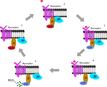
Figure 1: Activation cycle of G-proteins by G-protein-coupled receptors. When a ligand activates the receptor, a conformation change occurs in the receptor that exchanges GDP for GTP on the $\alpha$ subunit and this triggers the dissociation of the $\alpha$ subunit from $\beta\gamma$ dimer and the receptor. After the free $\alpha$ unit works on target proteins, GTP will be hydrolyzed to GDP. The GTPase activity is enhanced by binding of the RGS.

While the mechanism of G-protein signaling is highly conserved, the diversity of signaling targets is immense [27]. Thus, the ability to swiftly model the dynamics of G-protein signaling is advantageous to both drug development and basic research.

1.2 Modeling

Two recent studies use ODEs to model the receptor and ligand binding dynamics and the G-protein cycle. Yi. et. al. [29] used an ODEs model together with fluorescent resonance energy transfer (FRET) measurement to characterize the heterotrimeric G-protein cycle in yeast. Hao, et. al. [13] also used an ODEs model to indicate the role of Sst2, an RGS protein, in G-protein cycling.

In our study, we build four new models using the stochastic Pi-calculus, stochastic Petri Nets, the Kappa language, and Bio-PEPA. Furthermore, we show that we obtain consistent results when compared with the ODEs model of Yi, et. al. [29] (Fig. 5). The simulators for stochastic Petri Nets [21] and the Kappa language [11], Cell Illustrator and Cellucidate, respectively, have an interface which is intuitive for biologists, and the syntax of Bio-PEPA is close to the chemical reactions notation and relatively easy to use, unlike SPiM, which requires understanding of communications primitives and concurrent processes. In order to hide such communication details we develop a high level notation that uses terminology directly obtained from biological processes, and we show how to systematically translate a process in high level notation into a SPiM process. (See Section 4.). Kahramanogullari. et. al. [16] and Guerriero. et. al. [12] have provided the narrative languages for SPiM and Bio-PEPA, respectively. Our high level notation is an alternative to their narrative languages.

1.3 Outline

In Section 2, we show how to implement the model for the G-protein cycle using five different methods. In Section 3, we compare the simulation results from the different implementations. In Section 4, we introduce a high level notations and the translations from high level notation to chemical reactions and SPiM code. Section 5 contains our conclusions and a comparison of the simulation and modeling approaches of the five methods considered in Section 2.

2 Method

2.1 ODEs modeling

The ODEs modeling approach is a traditional method applied by biologists to explore dynamic biological processes by numerical integration. Yi. et. al.  [29] give a computational model of the G-Protein cycle by means of ordinary differential equations (ODEs). The individual reactions comprising the key dynamics of heterotrimeric G-proteins in yeast are represented, along with their rate constants, in Table 1.

Table 1: The reactions used to model the G-protein cycle and the corresponding rate constants (rate parameters) for each reaction (G-protein tutorial from www.MathWorks.com).

No.	Reaction	Rate Parameters
1	L + R $\leftrightarrow$ RL	$K_{RL}=2\cdot 10^{6}M^{-1}\cdot s^{-1}$, $K_{RLm}=1\cdot 10^{-2}s^{-1}$
2	Gd + Gbg $\rightarrow$ G	$K_{G1}=1s^{-1}$
3	RL + G $\rightarrow$ Ga + Gbg + RL	$K_{Ga}=1\cdot 10^{-5}s^{-1}$
4	R $\leftrightarrow$ null	$K_{Rd0}=4\cdot 10^{-4}s^{-1},K_{Rs}=4s^{-1}$
5	RL $\rightarrow$ null	$K_{Rd1}=4\cdot 10^{-3}s^{-1}$
6	Ga $\rightarrow$ Gd	$K_{Gd}=0.11s^{-1}$

Reaction No. 1 is receptor-ligand interaction which corresponds to the transition from step 2 to step 3 in Fig. 1. R represents receptor; L represents ligand; and RL represents receptor and ligand bound together. Reaction No. 2 is heterotrimeric G-protein formation which can be found in the transition from step 1 to step 2 in Fig. 1. Gd represents the deactivated $\alpha$ subunit, which is bound to GDP; Gbg represents the $\beta\gamma$ sub-complex, and G represents $\alpha$ bound to $\beta\gamma$ and GDP. Notice that from step 1 to 2, the $\alpha$ subunit also binds to the receptor. However, the original paper does not consider it as a species, and consequently the ODEs model does not reflect that binding. Reaction No. 3 is G-protein activation which corresponds to the transition from step 3 to step 4 in Fig. 1. After the ligand and receptor interact with each other, the $\alpha$ subunit will be activated and bound to GTP, and it will dissociate from the $\beta\gamma$ sub-complex. Ga represents the activated $\alpha$ subunit, which is bound to GTP. Reaction No. 4 is receptor synthesis and degradation. Reaction No. 5 is receptor-ligand degradation. Reaction No. 6 is G-protein inactivation which corresponds to the transition from step 5 to step 1 in Fig. 1.

The ODEs of the model are as follows:

1. d[R]/dt=$-K_{RL}[L][R]+K_{RLm}[RL]-K_{Rd0}[R]+K_{Rs}$;

2. d[RL]/dt=$K_{RL}[L][R]-K_{RLm}[RL]-K_{Rd1}[RL]$;

3. d[G]/dt=$-K_{Ga}[RL][G]+K_{G1}[Gd][Gbg]$;

4. d[Ga]/dt=$K_{Ga}[RL][G]-K_{Gd}[Ga]$;

5. d[Gd]/dt=$-K_{G1}[Gd][Gbg]+K_{Gd}[Ga]$;

6. d[Gbg]/dt=$K_{Ga}[RL][G]-K_{G1}[Gd][Gbg]$;

7. d[L]/dt=$-K_{RL}[L][R]+K_{RLm}[RL]$;

According to Table 1, derived from the reactions diagram from Yi. et. al. [29], there are seven species in the model. However, they only describe the first four equations. In order to have one differential equation for each species, we build the last three equations. They also provide two conservation relationships: $[Gbg]=Gt-[G]$ and $[Gd]=Gt-[G]-[Ga]$ which are satisfied by our simulations. (See Section 3).

2.2 Stochastic Pi-calculus modeling

Process algebras are formal languages originally designed to model complex reactive computer systems where heterogeneous agents interact concurrently exchanging information through communication channels. Because of the similarities between reactive computer systems and biological systems, process algebras have recently been used to model biological systems [7, 26].

The stochastic Pi-calculus [26] is a process algebra where stochastic rates are imposed on processes, allowing for more accurate description of biological systems [7]. A process can be depicted as a collection of interacting automata with two kinds of reactions: delay@r and interaction@r on ch. A delay is a spontaneous change of state performed by a single automaton at a specified reaction rate r. Interaction, on the other hand, consists of a send/receive handshake between two automata over a channel ch, written !ch for send and ?ch for receive. The channel ch has an associated reaction rate r. Reaction rates are used to determine stochastically the reaction to be executed next [6]. For our modeling, we use SPiM, an implementation of the stochastic Pi-calculus that can be used to run in-silico simulations displaying the change in the populations of different species over time [23].

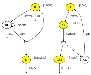
Figure 2: Graphical representation of Pi-calculus modeling

Fig. 2 depicts the stochastic Pi-calculus model we build for the G-protein cycle using SPiM. We divide the system into two parts that correspond to two viewpoints. The left hand side is the viewpoint of ligand and receptor, and the right hand side is the viewpoint of the G-protein. The initial numbers of different species are assigned in square brackets. For example, the initial concentration of R is 10000 and of G is 7000. Notice that RL and Ga are not initialized. All the reaction rates are also extracted from the literature [29] and continuous reactions are converted to discrete reactions according to standard rules[5]. For example, the pair !bindR/?bindR represents step 2 to 3 in Fig. 1, and it corresponds to reaction No. 1 in Table 1, and the pair !switch/?switch represents the step 3 to 4 in Fig. 1, and it corresponds to reaction No. 3 of Table 1. The corresponding SPiM code is in Table 2. The “directive plot” statement declares the species that will be plotted, in this case RL, G, and Ga. At the end of the program, each “run” statement declares the initial amount for different species. In the ODEs model, the amount of R is initialized to be 6.022E17 and the rate of the reaction No. 1 in Table 1 is 3.32E-18 with the assumed reaction volume 1 L ($M=mol\cdot L^{-1}$, $mol\cong 6.022\times 10^{23}$). Because simulating stochastic models is slower than solving ODEs, we scale the reaction volume down to 1.0E-12 L in order to speed up the stochastic simulation. Given this new reaction volume, the initial amount of R is 6.022E5, and the new reaction rate is 3.32E-6[5]. The other reaction rates remain unchanged, because they are discrete and do not depend on the volume. Assuming that pressure and temperature are unchanged, proportionally scaling reaction rates and reagent concentrations preserves the correctness of the modeling. We do not model the receptor generation aspect of reaction No. 4 in Table 1 (null $\rightarrow$ R), because on the one hand, this reaction is inconsequential to the whole system, as suggested by the result of Fig. 5, and on the other hand, the stochastic pi-calculus can not describe the generation of a process from the empty process. Furthermore, the initial amounts of receptor and G-protein guarantee abundance of receptor to enable the activation of G-protein. More details about our model can be found in the companion technical report [2].

Table 2: SPiM code for G-protein Cycle

directive sample 600.0	new bindR@rl:chan	and L()=( !bindR(); () )
directive plot RL(); G(); Ga()	new switch@ga:chan
		let Gd()= ( !bindb(); G() )
val rl = 3.32E-6	let R()=	and G()= ( ?switch(); (Ga() $\mid$ Gbg() ) )
val rlm= 0.01	(	and Ga()= ( delay@gd1; Gd())
val rs= 4.0	do ?bindR(); RL()	and Gbg()= ( ?bindb(); () )
val rd0= 4.0E-4	or delay@rd0; ()
val rd1= 4.0E-3	)	run 602200 of L()
val ga= 1.0E-5	and RL()=	run 10000 of R()
val gd1= 0.11	(	run 7000 of G()
val g1= 1.0	do delay@rlm; ( R() $\mid$ L() )	run 3000 of Gd()
	or delay@rd1; ()	run 3000 of Gbg()
new bindb@	or !switch(); RL() )

2.3 Petri Nets modeling

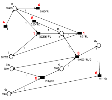
Figure 3: Petri Nets modeling

A Petri Net is a mathematical concept developed in the early 1960s by Carl Adam Petri to describe discrete distributed systems. Petri Nets are suitable for modeling and analyzing the dynamics of concurrent systems whose behavior could be described by finite sets of atomic processes and atomic states [21]. Petri Nets have subsequently been adapted and extended in many directions, including quantitative analysis of biological networks [25].

The basic Petri Net is a directed bipartite graph with two kinds of nodes which are either places or transitions and directed arcs which connect nodes. In modeling biological processes, place nodes represent molecular species and transition nodes represent reactions. We use Cell Illustrator to develop our model of the G-protein cycle (www.cellillustrator.com).

Fig. 3 is the Petri Net we build to model the G-protein cycle. Place nodes are represented as circles, and transition nodes are represented as boxes. The arcs are labeled with an integer weight, which represents the minimum value of input entities needed for the reactions to happen. The initial number of species and reaction rates can be read from the graph. For example, the initial amount of Receptor is 10000 and the initial amount of $\beta\gamma$ sub-complex is 3000, while Ga and RL are initialized to 0. Here we scale the reaction volume to be 1.0E-12 L, which is the same as in the SPiM model. The numbers in red correspond to the No. column in Table 1.

2.4 Kappa language modeling

Table 3: G-protein cycle is represented in Kappa language.

No.	Kappa Statement
1	R(r), L(l) $\leftrightarrow$ R(r!1), L(l!1) @ 3.32e-06,0.01
2	Gbg(bg), Gd(alpha $\sim$ GDP,a) $\rightarrow$ Gbg(bg!1), Gd(alpha $\sim$ GDP,a!1) @ 1.0
3	Gbg(bg!1), Gd(alpha $\sim$ GDP,a!1), R(r!2), L(l!2) $\rightarrow$ Gbg(bg),
	Gd(alpha $\sim$ GTP,a), R(r!1), L(l!1) @ 1.0e-05
4	R(r)$\leftrightarrow$ @4e-04,4
5	L(l!1), R(r!1) $\rightarrow$ @ 0.004
6	Gd(alpha $\sim$ GTP,a) $\rightarrow$ Gd(alpha $\sim$ GDP,a) @ 0.11

Kappa is a formal language for defining agents (typically meant to represent proteins) as sets of sites that constitute abstract resources for interaction. It is used to express rules of interactions between proteins characterized by discrete modification and binding states [11]. The Kappa language modeling platform Cellucidate is available at www.cellucidate.com.

In the Kappa language, reaction rules are described by rewriting rules between lists of agents. Each agent has a name and binding sites. For example, in R(r), R is the agent and r is its binding site. Agents can become bound, and the two end points of a link between two agents is indicated by !i, for some index i. $\sim$value specifies the internal state of a site on the agent, $\leftrightarrow$ specifies a bidirectional reaction, $\rightarrow$ specifies an unidirectional reaction, and @value specifies the reaction rate. For example,

R(r), L(l) $\leftrightarrow$ R(r!1), L(l!1) @ 3.32e-06,0.01

is a bidirectional reaction, where R and L are agent names, r is the binding site of R, l is the binding site of L; 0.01 is the reaction rate from left to right, and 3.32e-06 is the reaction rate from right to left. In R(r!1) and L(l!1), 1 is the index of the link that binds R and L at their binding sites. In our G-protein example, it corresponds to the binding of receptor and ligand. Gd( $\alpha$$\sim$GDP,a) represents the deactivated G-protein. $\sim$GDP represents the internal state of the $\alpha$ subunit where it is bound to GDP.

The Kappa language processes for the G-protein cycle are described in Table 3. The statements correspond to the reactions and rates in Table 1. The initial number of species can not be read from Table 3, but in fact, we use the same number as the Petri Nets model and SPiM model. For example the initial number for ligand is 6.022E5. Fig. 4 is the graphical representation of the processes described in Table 3 automatically generated by Cellucidate. $R+LRL$ means $R+L\rightarrow RL$, and $R+LRL\_op$ is the opposite direction: $R+L\leftarrow RL$. $NullR$ means $R\rightarrow null$, and $NullR\_op$ is the opposite direction: $R\leftarrow null$. The reactions with red arrows will consume R or RL, having a negative effect on the reaction $R+RL\rightarrow Ga+Gbg+RL$, while the green arrows have positive effects.

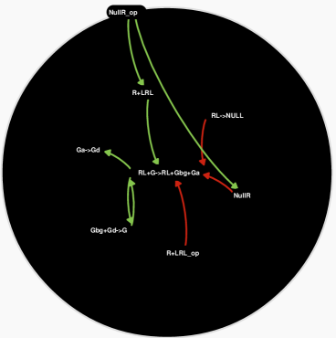
Figure 4: Graphical representation of Kappa language modeling

2.5 Bio-PEPA modeling

Bio-PEPA[10] is an extension of PEPA[14], which is specifically designed for modeling biochemical networks by explicitly defining the stoichiometry of reactions. The two existing tools for working with Bio-PEPA models are the Bio-PEPA Workbench and the Bio-PEPA Eclipse Plug-in[9]. We use the Bio-PEPA Eclipse Plug-in to model the G-protein Cycle, shown in Table 4. In Table 4, Parameter Definitions consist of rate constant declarations; Functional Rates are declarations of reaction names and the corresponding reaction rates. For example, in $kineticLawOfbindRL:fMA(rl)$, the name of the reaction is $bindRL$, the function for the law of Mass-Action is denoted by $fMA$, and $rl$ is the rate constant; under Species Components there is a representation of the reactions matching the corresponding differential equations of the ODEs model. For example,

$$G=bindAB>>G+activ<<G$$

indicates the role of reagent G in the related reactions. $bindAB>>G$ means $G$ is produced in reaction $bindAB$ and $activ<<G$ means $G$ is consumed in reaction $activ$. It also corresponds to

d[G]/dt=$-K_{Ga}[RL][G]+K_{G1}[Gd][Gbg]$,

where $g1$ is the rate constant of reaction $bindAB$, and $ga$ is the rate constant of reaction $activ$, corresponding to $K_{G1}$ and $K_{Ga}$ respectively.

Finally, the initial concentrations for each species are declared under Model Components. Because in our example the reactions are in the same cell, and the locations are the same for all species, the default location is used and left implicit.

The reaction rates and initial concentrations are all consistent with the other three models we built.

Table 4: Bio-PEPA code for G-protein Cycle

// Parameter Definitions

$rl=3.32E-6;$

$rlm=0.01;$

$ga=1.0E-5;$

$gd1=0.11;$

$g1=1.0;$

$rd1=4.0E-3;$

$rs=4.0;$

$rd0=4.0E-4;$

// Functional Rates

$kineticLawOfbindRL:fMA(rl);$

$kineticLawOfbindAB:fMA(g1);$

$kineticLawOfdisRL:fMA(rlm);$

$kineticLawOfactiv:fMA(ga);$

$kineticLawOfhydro:fMA(gd1);$

$kineticLawOfdegRL:fMA(rd1);$

$kineticLawOfdegR:fMA(rd0);$

$kineticLawOfproR:rs;$

// Species Components

$L=disRL>>L+bindRL<<L;$

$R=disRL>>R+bindRL<<R+degR<<R+proR>>R;$

$RL=disRL<<RL+bindRL>>RL+activ(+)RL+degRL<<RL;$

$G=bindAB>>G+activ<<G;$

$Ga=activ>>Ga+hydro<<Ga;$

$Gd=bindAB<<Gd+hydro>>Gd;$

$Gbg=bindAB<<Gbg+activ>>Gbg;$

// Model Components

$L[602200]<*>R[10000]<*>RL[0]<*>G[7000]$

$<*>Gd[3000]<*>Gbg[3000]<*>Ga[0]$

3 Simulation Results and Comparison

Although we are not proposing a theoretical comparison of the five modeling techniques, or the five implementations in different formalisms, we show here consistent experimental simulation results. SPiM, Cell Illustrator, Cellucidate, and Bio-PEPA all use Gillespie’s algorithm for simulation. Fig. 5 shows that the results from those four simulations are consistent with the result of the original ODEs modeling. The plots show that RL is consumed as the reaction proceeds. The curves of G and Ga decline and increase oppositely, and the sum of these two species is a constant, which is equal to the initial amount of G-protein, so the conservation relationships mentioned by Yi. et. al. are confirmed ($[Gbg]=Gt-[G]$, $[Gd]=Gt-[G]-[Ga]$) [29].

These computational models can be classified according to different properties.

Simulation Approach. The simulation approach can be stochastic or deterministic. While the deterministic approach is faster, the stochastic approach is more accurate. In particular, because of the randomness of dynamic biological systems, the stochastic approach can make the simulation of biological processes more faithful. Furthermore, while a deterministic system may get stuck into a specific state, stochastic noise allows the system to oscillate in and out of that state [28].

Our four models of the G-protein cycle in the stochastic Pi-calculus, stochastic Petri Nets, the Kappa language, and Bio-PEPA fall into the category of stochastic simulation, while the traditional ODEs model is deterministic.

Far from competing with each other, both modeling approaches are complementary, and often it is possible to derive one model from the other. In particular, Feret, et. al. show how to convert a rule-based model, such as a Kappa model, into a reduced systems of differential equations [11], Priami, et. al. show how to translate an ODEs model into a Stochastic Pi-calculus model [20], and Cardelli, et. al. show how to convert processes to ODEs [4].

Modeling Approach. The five models discussed here are either chemical reaction centric or process centric. The ODEs, Petri Nets, Kappa, and Bio-PEPA models are chemical reaction centric. In particular, Kappa takes a rule based approach that corresponds to high level chemical reactions. For each chemical reaction there is an equation, a transition or a rule in the corresponding model. On the other hand, the stochastic Pi-calculus model is process centric; there is one process for each component or observable product, leading to a much simpler model. Andrew Phillips shows the simplicity of the SPiM process model in contrast with the chemical reactions model [22].

While ODEs are low level and close to chemical reactions, Petri Nets constitute a graphical representation of chemical reactions. A SPiM model is a low level representation of individual protein behavior using send and receive communication primitives over a channel, and Kappa is a graphical high level abstraction of chemical reactions.

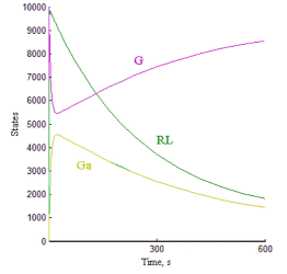
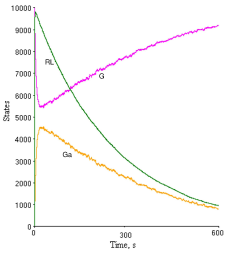
(a)	(b)
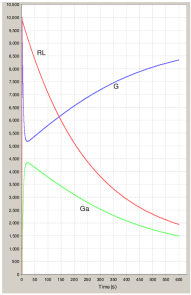
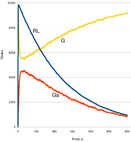
(c)	(d)
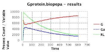
(e)

Figure 5: (a). Simulation result of ODEs model from MathWorks. (b). Simulation result of process model from SPiM. (c). Simulation result of Petri Nets model from Cell Illustrator. (d). Simulation result of Kappa language from Cellucidate. (e). Simulation result of Bio-PEPA from Eclipse Plug-in. In all five cases, RL represents receptor bound to ligand, Ga represents the activated G-protein, and G represents the deactivated G-protein. The x axis is time in seconds, and the y axis is intensity of states.

4 High Level Notation

Both ODEs and Petri Nets correspond closely to chemical reactions, and for the average biologist, they are relatively easy to understand. However, according to our experience in the classroom and in the lab, communicating with biology students and scientists, understanding the stochastic Pi-calculus, the Kappa language and Bio-PEPA (to a lesser extent) to be able to model molecular processes, requires a considerable initial effort. While Kappa has a user friendly graphical syntax available through Cellucidate. SPiM, on the other hand, still needs encoding in the stochastic Pi-calculus. To address this issue and enable modeling using descriptions directly obtained from biological processes, a narrative language has been proposed for SPiM [16]. Here we propose an alternative high level notation, and we show how to systematically translate it into SPiM programs and also chemical reactions.

Table 5: High Level Notation

Action A ::= bind(a, b, c, r) $\mid$ dimerize(a, b, c, r) $\mid$ activate(a, b, c, r) $\mid$ activateAnddissociate(a, b, c, d, r) $\mid$ phosphorylate(a, b, c, r) $\mid$ dissociate (a, b, c, r) $\mid$ degrade(a, r) $\mid$ hydrolyze(a, b, r) Process P ::= A; P $\mid$ ()

$\mbox{SPiM}($bind(a, b, c, r)$)=\{a\rightarrow^{!ch@r}c;b\rightarrow^{?ch@r}()\}=\mbox{SPiM}($dimerize(a, b, c, r)$)$ where ch is new $\mbox{SPiM}($phosphorylate(a, b, c, r)$)=\{a\rightarrow^{!ch@r}c;b\rightarrow^{?ch@r}b\}$ where ch is new $\mbox{SPiM}($dimerize(a, b, c, r)$)=\{a\rightarrow^{!ch@r}c;b\rightarrow^{?ch@r}()\}=\mbox{SPiM}($bind(a, b, c, r)$)$ where ch is new $\mbox{SPiM}($activate(a, b, c, r)$)=\{a\rightarrow^{!ch@r}c;b\rightarrow^{?ch@r}b\}$ where ch is new $\mbox{SPiM}($activateAnddissociate(a, b, c, d, r)$)=\{a\rightarrow^{!ch@r}c\ \mid\ d\ ;b\rightarrow^{?ch@r}b\}$ where ch is new $\mbox{SPiM}($dissociate(a, b, c, r)$)=\{a\rightarrow^{delay@r}b\hskip 5.0pt\mid\hskip 5.0ptc\}$ $\mbox{SPiM}($hydrolyze(a, b, r)$=\{a\rightarrow^{delay@r}b\}$ $\mbox{SPiM}($degrade(a, r)$=\{a\rightarrow^{delay@r}()\}$

SPiM* (()) = $\emptyset$ SPiM* (A; P) = SPiM(A) $\cup$ SPiM* (P)

Table 6: Translation of High Level Notation into Chemical Reactions

$\mbox{Reaction}($bind(a, b, c, r)$)=a+b\rightarrow^{r}c$ $\mbox{Reaction}($phosphorylate(a, b, c, r))$)=a+b\rightarrow^{r}c+b$ $\mbox{Reaction}($dimerize(a, b, c, r)$)=a+b\rightarrow^{r}c$ $\mbox{Reaction}($activate(a, b, c, r)$)=a+b\rightarrow^{r}c+b$ $\mbox{Reaction}($activateAnddissociate(a, b, c, d, r)$)=a+b\rightarrow^{r}c+d+b$ $\mbox{Reaction}($dissociate(a, b, c, r)$)=a\rightarrow^{r}b+c$ $\mbox{Reaction}($hydrolyze(a, b, r))$)=a\rightarrow^{r}b$ $\mbox{Reaction}($degrade(a, r)$)=a\rightarrow^{r}null$

Reaction* (()) = $\emptyset$ Reaction* (A; P) = Reaction(A) $\cup$ Reaction* (P)

We write a, b, c, d, etc. for species, r for reaction rate constants, A for actions, and P for a process consisting of a possibly empty sequence of actions. Table 5 shows a list of actions representing familiar biological processes. bind(a, b, c, r) means two reagents a and b bind together to generate the product c at rate r. Similarly, dimerize(a, b, c, r) means that a and b form a dimer denoted by c at rate r. dissociate(a, b, c, r) is the opposite action to bind(a, b, c, r); a is broken down into b and c at rate r. activate(a, b, c, r) and activateAnddissociate(a, b, c, d, r) basically represent the same biological process where the reagent a becomes activated in the presence of another reagent b at rate r. The difference is that activate only generates the activated state product c while activateAnddissociate generates the activated product, and the product simultaneously dissociates into two products c and d. phosphorylate(a, b, c, r) represents phosphorylation at rate r, where a is the protein reagent, b is the kinase, and c is the product. hydrolyze(a, b, r) represents the hydrolysis at rate r, where a is the reagent and b is the product. degrade(a, r) means a degrades at rate r. Notice that bind(a, b, c, r) and dimerize(a, b, c, r) are basically the same operation, but in order to distinguish these two different biological processes, we have two names. In biology, dimerization is the binding which can generate a dimer.

Table 5 also defines the translation function SPiM, that given an action in high level notation returns the corresponding SPiM process, and SPiM*, its homomorphic extension to processes. To aide readability, instead of using stochastic Pi-calculus code, we use the equivalent graph representation of SPiM processes [8]. Similarly, Table 6 defines the translation functions Reaction and Reaction* that translate processes in high level notation into chemical reactions.

Going back to our G-Protein example in Fig. 1, bind(Gd, Gbg, G, 1.0) corresponds to step 1 to 2, bind(R, L, RL, 3.32e-6) to step 2 to 3, activateAnddissociate(G, RL, Ga, Gbg, 1.0e-5) to the activation in steps 2 to 3 and the dissociation in step 3 to 4, dissociate(RL, R, L, 0.01) represents step 4 to 5 and hydrolyze(Ga, Gd, 0.11); degrade(R, 4e-4); degrade(RL, 4e-3) correspond to step 5 to 1 completing the cycle.

The translation of the high level notation of the G-protein cycle into SPiM is as follows:

$$\begin{array}[]{l}\textbf{SPiM*(bind(Gd, Gbg, G, 1.0); bind(R, L, RL, 3.32e-6);}\\ \textbf{activateAnddissociate(G, RL, Ga, Gbg,1.0e-5); dissociate(RL, R, L, 0.01);}\\ \textbf{hydrolyze(Ga, Gd, 0.11); degrade(R, 4e-4); degrade(RL, 4e-3))}\\ =\\ \{Gd\rightarrow^{!bindb@1.0}G;Gbg\rightarrow^{?bindb@1.0}()\}\cup\textbf{SPiM*(bind(R, L, RL, 3.32e-6);}\\ \textbf{activateAnddissociate(G, RL, Ga, Gbg,1.0e-5); dissociate(RL, R, L, 0.01);}\\ \textbf{hydrolyze(Ga, Gd, 0.11); degrade(R, 4e-4); degrade(RL, 4e-3))}\\ =\\ \quad$\vdots$\\ =\\ \{Gd\rightarrow^{!bindb@1.0}G;Gbg\rightarrow^{?bindb@1.0}()\}\cup\{R\rightarrow^{!bindR@3.32e-6}RL;L\rightarrow^{?bindR@3.32e-6}()\}\cup\\ \{G\rightarrow^{?switch@1.0e-5}Ga\ \mid\ Gbg\ ;RL\rightarrow^{!switch@1.0e-5}RL\}\cup\{RL\rightarrow^{delay@{0.01}}R\ \mid\ L\}\cup\\ \{Ga\rightarrow^{delay@{0.11}}Gd\}\cup\{R\rightarrow^{delay@{4e-4}}()\}\cup\{RL\rightarrow^{delay@{4e-3}}()\}\end{array}$$

Finally, the translation of the high level notation of the G-protein cycle into chemical reactions is as follows:

$$\begin{array}[]{l}\textbf{Reaction*(bind(Gd, Gbg, G, 1.0); bind(R, L, RL, 3.32e-6);}\\ \textbf{activateAnddissociate(G, RL, Ga, Gbg,1.0e-5); dissociate(RL, R, L, 0.01);}\\ \textbf{hydrolyze(Ga, Gd, 0.11); degrade(R, 4e-4); degrade(RL, 4e-3))}\\ =\\ Gd+Gbg\rightarrow^{1.0}G\cup\textbf{Reaction*(bind(R, L, RL, 3.32e-6);}\\ \textbf{activateAnddissociate(G, RL, Ga, Gbg,1.0e-5); dissociate(RL, R, L, 0.01);}\\ \textbf{hydrolyze(Ga, Gd, 0.11); degrade(R, 4e-4); degrade(RL, 4e-3))}\\ =\\ \quad$\vdots$\\ =\\ Gd+Gbg\rightarrow^{1.0}G\cup R+L\rightarrow^{3.32e-6}RL\cup\\ G+RL\rightarrow^{1.0e-5}Ga+Gbg+RL\cup RL\rightarrow^{0.01}R+L\cup\\ Ga\rightarrow^{0.11}Gd\cup R\rightarrow^{4e-4}null\cup RL\rightarrow^{4e-3}null\end{array}$$

Kahramanogullari. et. al. [16], propose a narrative language that is translated into a model with three kinds of sentences (association, dissociation and transformation), where species have explicit binding sites (as in Kappa). They also show how to translate models into SPiM and how to obtain a model using the narrative language. Our high level notation is an alternative to their narrative language, however we translate it directly into SPiM, and we do not need a notion of model. In their example of Appendix A, the generated code for processes FcR2 and FcR3, for example, does not correspond to any species in the biological example being modeled.

5 Conclusion

Although building computational models of cellular processes is not new, to the best of our knowledge, this is the first time that a model has been implemented in five different formalisms. Furthermore, our classroom experience shows that this survey paper is a valuable tutorial introduction to bio-modeling in these diverse frameworks. In order to make a formal comparison for all five formalisms, one would need to define translation functions between the different formalisms and a notion of correctness for each translation.

Starting from an exiting ODEs model of the activation cycle of G-proteins by G-protein coupled receptors, we construct four simulations in four different formalisms: Stochastic Pi-Calculus, Stochastic Petri Nets, Kappa, and Bio-PEPA. We also show how to scale initial concentrations and reaction rates for this specific example to compensate for the fact that solving differential equations in MatLab is faster than executing a concurrent model.

Finally, our high level notation is an abstraction for both SPiM and chemical reactions. Our high level notation corresponds to commonly-occurring reaction schemes easily identifiable by biologists, and it is an alternative to the narrative language proposed for SPiM. Our high level notation represents the G-protein cycle quite concisely, it is accessible to the average biologist, and it translates naturally into SPiM and chemical reactions, suggesting that our models could be effective instruments to assist in biomedical research.

This notation naturally induces a typed modeling language that is currently being explored, where a,b $\vdash$ bind@r;P reduces to complex(a,b) $\vdash$ P, where complex is only defined for specific species, for example.

References

- [1]
- [2] Yifei Bao, Tommy White, Joseph Glavy & Adriana Compagnoni (2010): Application of SPiM to Process Modeling for the Activation Cycle of G-proteins by G-protein-coupled Receptors. Technical Report CS-2010-1, Stevens Institute of Technology.
- [3] Jo l Bockaert, Philippe Marin, Aline Dumuis & Laurent Fagni (2003): The ‘magic tail’ of G Protein-Coupled Receptors: An Anchorage for Functional Protein Networks. FEBS Letters 546(1), pp. 65–72. Signal Transduction Special Issue.
- [4] Luca Cardelli (2008): From Processes to ODEs by Chemistry. In: IFIP TCS, pp. 261–281.
- [5] Luca Cardelli (2008): On Process Rate Semantics. Theor. Comput. Sci. 391(3), pp. 190–215.
- [6] Luca Cardelli (2009): Artificial Biochemistry. In: Anne Condon, David Harel, Joost N. Kok, Arto Salomaa & Erik Winfree, editors: Algorithmic Bioprocesses, Natural Computing Series, Springer Berlin Heidelberg, pp. 429–462.
- [7] Luca Cardelli, Emmanuelle Caron, Philippa Gardner, Ozan Kahramanogullari & Andrew Phillips (2009): A Process Model of Actin Polymerisation. Electr. Notes Theor. Comput. Sci. 229(1), pp. 127–144.
- [8] Luca Cardelli, Emmanuelle Caron, Philippa Gardner, Ozan Kahramanogullari & Andrew Phillips (2009): A Process Model of Rho GTP-binding Proteins. Theor. Comput. Sci. 410(33-34), pp. 3166–3185.
- [9] Federica Ciocchetta, Adam Duguid, Stephen Gilmore, Maria Luisa Guerriero & Jane Hillston (2009): The Bio-PEPA Tool Suite. Quantitative Evaluation of Systems, International Conference on 0, pp. 309–310.
- [10] Federica Ciocchetta & Jane Hillston (2009): Bio-PEPA: A framework for the Modelling and Analysis of Biological Systems. Theoretical Computer Science 410(33-34), pp. 3065–3084.
- [11] Jérôme Feret, Vincent Danos, Jean Krivine, Russ Harmer & Walter Fontana (2009): Internal Coarse-graining of Molecular Systems. Proceedings of the National Academy of Sciences 106(16), pp. 6453–6458.
- [12] Maria Luisa Guerriero, John K. Heath & Corrado Priami (2007): An Automated Translation from a Narrative Language for Biological Modelling into Process Algebra. In: CMSB, pp. 136–151.
- [13] Nan Hao, Necmettin Yildirim, Yuqi Wang, Timothy C. Elston & Henrik G. Dohlman (2003): Regulators of G Protein Signaling and Transient Activation of Signaling: Experimental and computational analysis reveals negative and positive feedback controls on g protein activity. J. Biol. Chem. 278(47), pp. 46506–46515.
- [14] Jane Hillston (1996): A Compositional Approach to Performance Modelling. Cambridge University Press, New York, NY, USA.
- [15] Andrew D. Howard, George McAllister, Scott D. Feighner, Qingyun Liu, Ravi P. Nargund & Lex H. T. Van der Ploeg an (2001): Orphan G-protein-coupled Receptors and Natural Ligand Discovery. Trends in Pharmacological Sciences 22(3), pp. 132–140.
- [16] Ozan Kahramanogullari, Luca Cardelli & Emmanuelle Caron (2009): An Intuitive Automated Modelling Interface for Systems Biology. CoRR abs/0911.2327.
- [17] Brian K. Kobilka (2007): G Protein Coupled Receptor Structure and Activation. Biochim Biophys Acta 1768(4), pp. 794–807.
- [18] Louis M. Luttrell (2006): Transmembrane Signaling Protocols, chapter Transmembrane Signaling by G Protein-Coupled Receptors, pp. 3–49. Humana Press.
- [19] William M. Oldham & Heidi E. Hamm (2008): Heterotrimeric G protein Activation by G-protein-coupled Receptors. Nat Rev Mol Cell Biol 9(1), pp. 60–71.
- [20] Alida Palmisano, Ivan Mura & Corrado Priami (2009): From ODES to Language-based, Executable Models of Biological Systems. Pacific Symposium on Biocomputing 14(12), pp. 239–250.
- [21] Mor Peleg, Daniel Rubin & Russ B. Altman (2005): Using Petri Net Tools to Study Properties and Dynamics of Biological Systems. Journal of the American Medical Informatics Association 12(2), pp. 181–199.
- [22] Andrew Phillips (2009): Symbolic Systems Biology: Theory and Methods, chapter A Visual Process Calculus for Biology. Jones and Bartlett. In Press.
- [23] Andrew Phillips & Luca Cardelli (2007): Efficient, Correct Simulation of Biological Processes in the Stochastic Pi-calculus. In: Computational Methods in Systems Biology, LNCS 4695, Springer, pp. 184–199.
- [24] Kristen L. Pierce, Richard T. Premont & Robert J. Lefkowitz (2002): Seven-transmembrane Receptors. Nat Rev Mol Cell Biol 3(9), pp. 639–650.
- [25] John W. Pinney, David R. Westhead & Glenn A. McConkey (2003): Petri Net representations in Systems Biology. Biochem. Soc. Trans. 31(6), pp. 1513–1515.
- [26] Corrado Priami, Aviv Regev, Ehud Y. Shapiro & William Silverman (2001): Application of A Stochastic Name-passing Calculus to Representation and Simulation of Molecular Processes. Inf. Process. Lett. 80(1), pp. 25–31.
- [27] Janet D. Robishaw & Catherine H. Berlot (2004): Translating G protein Subunit Diversity Into Functional Specificity. Current Opinion in Cell Biology 16(2), pp. 206–209.
- [28] José M. G. Vilar, Hao Yuan Kueh, Naama Barkai & Stanislas Leibler (2002): Mechanisms of Noise-resistance in Genetic Oscillators. PNAS 99(9), pp. 5988–5992.
- [29] Tau M. Yi, Hiroaki Kitano & Melvin I. Simon (2003): A Quantitative Characterization of The Yeast Heterotrimeric G Protein Cycle. Proc Natl Acad Sci U S A 100(19), pp. 10764–9.