Effect of quasi-bound states on coherent electron transport in twisted nanowires

Abstract

Quantum transmission spectra of a twisted electron waveguide expose the coupling between traveling and quasi-bound states. Through a direct numerical solution of the open-boundary Schrödinger equation we single out the effects of the twist and show how the presence of a localized state leads to a Breit-Wigner or a Fano resonance in the transmission. We also find that the energy of quasi-bound states is increased by the twist, in spite of the constant section area along the waveguide. While the mixing of different transmission channels is expected to reduce the conductance, the shift of localized levels into the traveling-states energy range can reduce their detrimental effects on coherent transport.

I Introduction

Conductance spectra of quasi-1D semiconductor structures display many features that expose directly the quantum nature of carrier transport, and are of great interest both for applications and fundamental understandingsIhn (2004); Rurali (2010). Even in the simplest non-interacting carriers approach, the departure from a constant section of the wire gives rise to complex resonance patterns in the quantum transmission. This originates from the coherent coupling of the energy spectra of different subbands and from the interplay of traveling and localized statesNöckel and Stone (1994). Indeed, the case of a discrete energy spectrum merged with a continuum one, was considered by FanoFano (1961) in his seminal work on inelastic scattering amplitudes of electrons. In that case, the two Hamiltonians with discrete and continuous spectra were that of the electronic degree of freedom of an atom and that of a free electron, respectively. It was shown that the coupling induced by the Coulomb interaction led to a peculiar asymmetric shape of the scattering probability and a discontinuity of the scattering phase. This behavior of the scattering amplitude is now identified in many atomicFransson and Balatsky (2007), opticalRotter et al. (2004) and transportGöres et al. (2000) experiments (for a review see Ref. Miroshnichenko et al., 2010).

Here, we analyze the coherent transmission of a quantum waveguide (QW) locally twisted, as depicted in Fig. 1, with the twist inducing a coupling between the subbands related to different transverse modes.

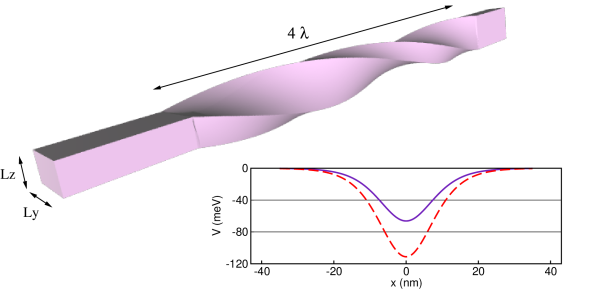
Figure 1: Quantum waveguide with rectangular cross-section ($L_{y}=20$ nm, $L_{z}=10$ nm) twisted for a length of $4\lambda\simeq 70$ nm. Here the rotation angle is $\Phi=\frac{3}{2}\pi$. Inset: local confining potential, as given in Eq. (3), with $L_{p}=10$ nm and $\nu=2.95$ (solid line) or $\nu=3.95$ (dashed line). The potential well is fully contained in the twisted region.

A local attractive potential is also included, in order to give rise to a discrete set of bound states and to Fano resonances in the transmission spectra: they will expose the energy of quasi-bound states of the twisted QW. We stress that our results are representative of a more general case, as for example a carrier scattered through a quantum dot embedded in a QW or a QW whose Hamiltonian is not separable in the transverse and longitudinal directions, leading to localized states.

The effect of twisting on the conductance is twofold. On one side, it is expected to reduce the conductanceSuzuura (2006); Tseng et al. (2009). On the other side, this reduction can be compensated by a partial destruction of localization effects (e.g. due to external fields or impurities), induced by the twisting itself. In fact, by means of the complex scaling method it has been shownKovařík and Sacchetti (2007) that stable states associated to a trapping potential may become resonant states when the QW is twisted. In this paper we numerically compute the real and imaginary part of such resonances as a function of the twisting parameter in an explicit model and we prove that, for such a model, the imaginary part of these resonances actually takes a negative value, this indicating that the corresponding states become unstable. Specifically, our results show that the energy of bound states of the quantum well in the longitudinal direction is increased by the twist and, as they enter the continuous-spectrum range of traveling states, they appear in the the transmission characteristic as symmetric (Breit-Wigner Breit and Wigner (1936)) or asymmetric (Fano Fano (1935)) resonant peaks, according to the character of the original bound wave function. The width of the resonances is related to the imaginary component of the eigenvalues of the complex-scaled Hamiltonian Reinhardt (1982), as we detail in the following, and shows a non-monotonic behavior. A resonant peak may or may not disappear when its energy reaches the transmission channel with the same transverse energy as the original bound state, according to the corresponding bound state in the straight QW. Indeed, the knowledge of the bound states of the straight QW allows one to predict the position and type of transmission resonances in the twisted system.

Our work is organized as follows. In Sect. II we describe the model of the twisted QW and, in the following Sect. III, we outline the real-space numerical approach adopted for the calculation of the scattering states and transmission amplitudes on a non-Cartesian grid. In Sect. IV the main results of our study are presented, with particular attention to the evolution of resonant peaks with the QW twist. Finally, in Sect. V we draw our conclusions. In the final Appendix, analytical details of the complex-scaling approach mentioned in the main text, are given.

II The physical system

We consider a QW with rectangular cross-section, with an hard-wall confinement. For a straight wire, an elementary solution of the single-band effective-mass Schrödinger equation gives the energy spectrum

$$E_{n,k}=E_{n}+\frac{\hbar^{2}}{2m}k^{2},$$ (1)

with

$$E_{n}=\frac{\hbar^{2}}{2m}\left[\left(\frac{n_{y}\pi}{L_{y}}\right)^{2}+\left(\frac{n_{z}\pi}{L_{z}}\right)^{2}\right],$$ (2)

where $m$ is the effective mass of the carrier, $L_{y}$ and $L_{z}$ (with $L_{y}\neq L_{z}$) are the thicknesses of the QW in the two directions orthogonal to the current propagation, $k$ is the wave number of the $x$-propagating plane wave component of the wave function. For the sake of brevity, the subband index $n=1,2,\dots$ (with $E_{n,k}\leq E_{(n+1),k}$) has been introduced, summarizing the two positive integers $n_{y}$ and $n_{z}$. Since $k$ can be any real number, it is clear that the energy spectrum is continuum, with $E_{n,k}\in[E_{1}\,,+\infty)$.

A confining potential well (depicted in Fig. 1 inset) is introduced along the $x$ direction

$$V\left(x\right)=\frac{\hbar^{2}}{2m}\frac{\nu\left(\nu+1\right)}{L_{p}^{2}}\left[\tanh^{2}\left(\frac{x}{L_{p}}\right)-1\right],$$ (3)

where the positive parameters $\nu$ and $L_{p}$ set the depth and the length of the well. Specifically, the minimum of $V$ is $-\hbar^{2}\nu\left(\nu+1\right)/(2mL_{p}^{2})$, and the region in which $V$ is significantly different from zero is about $6\,L_{p}$. We stress that the form given in Eq. (3) has been chosen both to mimic a “smooth” local confinement and to deal with a potential that has an exact expression for its bound-state eigenvalues Morse and Feshbach (1953):

$$\mu_{j}=-\frac{\hbar^{2}}{2mL_{p}^{2}}\left(\nu+1-j\right)^{2},\;j=1,2,\ldots,\lceil\nu\rceil\,,$$ (4)

where the ceiling function $\lceil\nu\rceil$ indicates the smallest integer not less than $\nu$. The above expression is essential to approach analytically the problem through the complex scaling method, that we use to follow the energy vs. twist behavior of the bound states.

The energetic spectrum of the Schrödinger operator for the QW with $V$ consists of a discrete and a continuum part

$$\left\{E_{n}+\mu_{j};\,n=1,2,\ldots;\,j=1,\ldots,\lceil\nu\rceil\right\}\cup[E_{1}\,,+\infty).$$ (5)

For energies above $E_{1}$ the two parts overlap and eigenvalues of the discrete spectrum are embedded in the continuum spectrum. However, the two sub-spectra remain well distinct since the system Hamiltonian is separable in a transverse ($y$-$z$ plane) and a longitudinal ($x$ direction) component. In fact, if a given energy corresponds to a discrete level and, at the same time, it lies inside the continuum, the corresponding state will be degenerate, with the different eigenfunctions having a different transverse state. In terms of quantum transport along the QW, the above system does not mix different transmission channels or propagating states with bound ones.

Let us now introduce a local twist in the QW. As we will show, this couples different transverse modes, mixing their spectra, and shifts the energy of the discrete states. The deformation adopted, also illustrated in Fig. 1, is a rotation of the rectangular cross-section around its center when moving along the QW axis. A point of coordinates $(x,y,z)$ of the straight QW is transformed according

$$x^{\prime} = x,$$

$$y^{\prime} = y\cos\left[\varphi\left(x\right)\right]+z\sin\left[\varphi\left(x\right)\right],$$ (6)

$$z^{\prime} = z\cos\left[\varphi\left(x\right)\right]-y\sin\left[\varphi\left(x\right)\right],$$

where

$$\varphi\left(x\right)=\frac{\Phi}{2}\left[\textrm{erf}\left(\frac{x}{\lambda}\right)+1\right]$$ (7)

is the rotation angle as a function of the longitudinal position $x$. Here, erf is the error function, $\Phi$ is the total rotation angle, and $\lambda$ is a parameter that sets the length of the twisted region. In particular, the QW twist can be considered effective in a length $4\,\lambda$ around the origin. Outside the latter region, the QW is essentially straight.

For our simulations, we use GaAs effective electron mass $m=0.067\,m_{e}$ and adopt the following set of geometric parameters: $L_{y}=20$ nm, $L_{z}=10$ nm, $\lambda=17.5$ nm (i.e. the twisted region is about $70$ nm), $0\leq\Phi\leq 3\pi$. Two attractive potentials, as given in Eq. (3), have been used, both with $L_{p}=10$ nm (i.e. effective on a length of about $60$ nm around the origin). They differ by their depth: in the first case $\nu=2.95$ (corresponding to a minimum of $-66.262$ meV), in the second case $\nu=3.95$ (corresponding to a minimum of $-111.186$ meV). The relative positions of relevant energy levels are reported in Fig. 2, for the two cases.

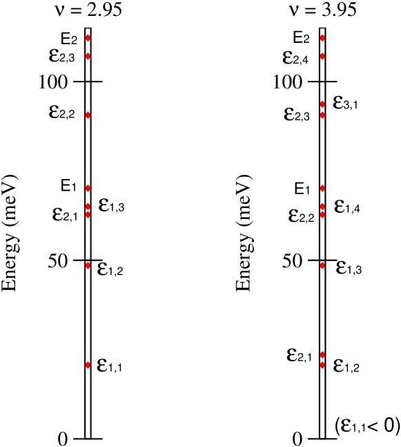
Figure 2: Schematic representation of the relevant energies of the system without twist for two different magnitudes of the quantum well described by Eq. (3). The thresholds of the transport channels, i.e. the transverse modes, are $E_{1}=70.155$ meV, $E_{2}=112.248$ meV, $E_{3}=182.403$ meV (not shown). The energy of a bound state of the straight QW is indicated with $\varepsilon_{n,j}$, with $n$ indicating the transverse mode, and $j$ the bound state of $V$ in the longitudinal direction. While the $E_{n}$’s are fixed, the $\varepsilon_{n,j}$’s are increased by the twist.

For brevity, the energies of the discrete states are indicated by $\varepsilon_{n,j}=E_{n,0}+\mu_{j}$ in the following. We stress that the transverse energies $E_{n}$ are fixed, since the cross-section is constant, although rotated. Contrary, the position of $\varepsilon_{n,j}$ depends upon the twist, as we will analyze in detail in Section IV. In fact, they are the resonant energies that correspond to a local maximum (Breit-Wigner) or a zero (Fano) in the transmission spectra.

III Numerical approach

To obtain the transmission amplitudes of the twisted QW we solve the 3D Schrödinger equation with open boundaries through the quantum transmitting boundary method Lent and Kirkner (1990) (QTBM). Electrons are injected from the left lead (see Fig. 1) in a given transverse mode, and can be either reflected or transmitted to the right lead. With this boundary condition, the differential equation of motion is solved in the internal points of the domain, leading to complex transmission/reflection amplitudes for every channel of the right/left leads. We adopt a curved coordinate system naturally defined by the twist function of Eq. (II) $\mathbf{r}=(x,y,z)\to\mathbf{r^{\prime}}=(x^{\prime},y^{\prime},z^{\prime})$. This new coordinate system follows the QW twist and “sees” a straight QW. However, also the equation of motion must be transformed according to the $\mathbf{r}\to\mathbf{r^{\prime}}$ relation. In order to do so, we need the metric tensor of the system $\mathbf{G}(\mathbf{r})$ with components $G_{ij}(\mathbf{r})=(\partial_{i}\mathbf{r^{\prime}})\cdot(\partial_{j}\mathbf{r^{\prime}})$, together with its inverse $\mathbf{G}^{-1}$ with components $G^{ij}$. Here, we used the definitions $\partial_{i}=\partial/\partial x^{i}$ and $(x,y,z)=(x^{1},x^{2},x^{3})$. In the curved coordinate system the Hamiltonian reads da Costa (1981); Ferrari and Cuoghi (2008):

$$\mathcal{H}(\mathbf{r})=-\frac{\hbar^{2}}{2m}\sum_{i,j=1}^{3}\frac{\partial_{i}}{\sqrt{G}}\left(\sqrt{G}G^{ij}\partial_{j}\right)$$

$$=-\frac{\hbar^{2}}{2m}\sum_{i,j=1}^{3}\left[G^{ij}\partial^{2}_{ij}-\left(\sum_{k,l=1}^{3}G^{kl}\partial^{2}_{kl}\mathbf{r^{\prime}}\cdot G^{ij}\partial_{i}\mathbf{r^{\prime}}\right)\partial_{j}\right],$$

where $G>0$ is the determinant of $\mathbf{G}$ and $\partial^{2}_{ij}=\partial_{i}\partial_{j}$. Now it is easy to define a rectangular mesh following the QW in the new coordinate system, and discretize $\mathcal{H}$ through a finite-difference scheme. The corresponding Schrödinger equation $\mathcal{H}\psi=E\psi$ is then solved, with open boundary conditions at the two edges of the QW, as described above. The QTBM takes as an input the kinetic energy $E-E_{n}>0$ of the incoming electron and the wave function of the transverse mode $n$, and gives as an output the transmission/reflection amplitudes in the different channels Cuoghi et al. (2009). For this reason, a new calculation must be performed for every $E$ in a chosen set over the range of interest, with $E>E_{n}$.

Actually, in order to find the resonances we also used a complementary technique: the complex scaling approach described in Appendix Kovařík and Sacchetti (2007). This method leads to a complex-eigenvalue problem that allows one to identify in a straightforward way the resonances originated by the bound states of $V$. Moreover, it gives the energy levels of bound states below $E_{1}$, not achievable with the QTBM. In fact, the QTBM gives the transmission amplitude of the different transverse modes as a function of the carrier energy, and the position of transport resonances must be detected subsequently, as a relevant peak or dip in the transmission probability and as a continuum (abrupt) phase shift for a Breit-Wigner (Fano) resonance. However, the complex scaling method results to be very demanding from the computational point of view and we used its results only as a reference for specific cases. We leave the comparison of the two methods to a subsequent work.

IV Transmission spectra

As anticipated in Section II the transmission spectra of the straight QW can be obtained from a one-dimensional equation of motion with the potential $V$. In order to mix transmission channels, the transverse/longitudinal separability must be lifted. However, a generic deformation of the QW section along the wire, not only couples different transverse modes, but also introduces additional resonant energies, as in the case of a closed cavity attached at a side Price (1992); W. Porod and Lent (1992). This can make difficult to expose the sole effect of the coupling between the continuum and discrete spectra. For this reason, as well as for technological relevance, we choose a kind of deformation that does not alter the shape of the QW cross section, but only its orientation, and does not introduce further resonances. In fact, the QW twist has only two effects: first, it couples the transmission channels so that the transmission probability for a carrier injected in a given transverse mode also has traces of quasi-bound states of different modes; second, it increases the energies of quasi-bound states.

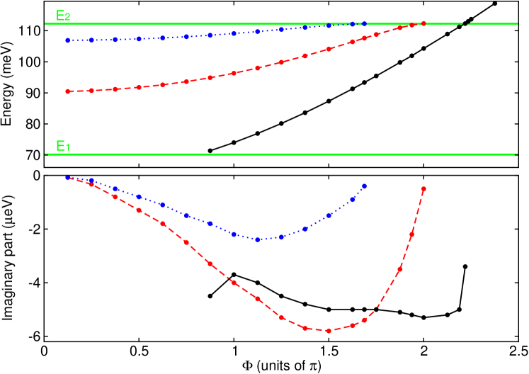
Figure 3: Top panel: position of transmission resonances in the ground-mode spectrum as a function of the twist angle $\Phi$, for $\nu=2.95$. The resonant energies correspond to the real part of the complex-scaled eigenvalues. The threshold energies of the ground and first-excited transverse modes are indicated by the two horizontal lines labeled as $E_{1}$ and $E_{2}$, respectively. The three curves correspond to the quasi-bound states $\epsilon_{2,3}$ (dotted line), $\epsilon_{2,2}$ (dashed line), $\epsilon_{2,1}$ (solid line). Bottom panel: Imaginary part of the complex-scaled eigenvalues, corresponding to the half width of the resonance peaks or dips. While the two Fano resonances $\epsilon_{2,3}$ and $\epsilon_{2,2}$ (see also Fig. 4) disappear as they reach $E_{2}$, $\epsilon_{2,1}$ is still present in the spectrum at energies exceeding $E_{2}$ in the form of a broad and shallow dip (see also Fig. 5).

These effects can be seen from the two panels of Fig. 3, where we report the position (top panel) and width (bottom panel) of the resonances in the transmission spectrum of the ground transverse channel, as a function of the twist angle. In particular, for each angle $\Phi$ we inject a carrier in the ground transverse mode (with energy $E_{1}$) and with several longitudinal kinetic energies, from zero to $E_{2}-E_{1}$. From the curves of transmission amplitude vs. total energy $E$ (see e.g. Figs. 4 and 5) we determine the position of the resonances and obtain the imaginary part of the eigenvalue as $-\Gamma/2$, where $\Gamma$ is the peak or dip width. Note that the above complex eigenvalues correspond to quasi-bound states with a mean lifetime $\hbar/\Gamma$ of the order of $100$ ps.

By comparing Fig. 3 with the levels of the straight QW given in Fig. 2, the origin of the two resonances at higher energy (dotted and dashed lines in Fig. 3) is clear. In fact, for $\Phi\sim 0$ only two quasi-bound levels lie between $E_{1}$ and $E_{2}$, namely $\epsilon_{2,2}$ and $\epsilon_{2,3}$. They both belong to channel $2$ so that at zero twist, they do not appear in the transmission spectrum, as it can be gathered from the vanishing imaginary part of their eigenvalue in the bottom panel of Fig. 3. As the twist is introduced, the two levels above appear as slightly asymmetric Fano dips in the transmission probability, as reported in the top panels of Fig. 4 for the case of $\Phi=\pi/2$. However, the Fano character of the resonances is better revealed by the abrupt jump of $\pi$ in the transmission phase $\theta$, as shown in the bottom panels of Fig. 4.

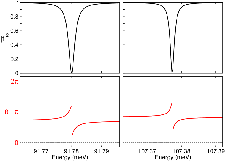
Figure 4: Ground-mode transmission probability (upper panels) and phase (lower panels) around the resonances $\epsilon_{2,2}$ (left panels) and $\epsilon_{2,3}$ (right panels) for a twist angle $\Phi=\pi/2$. In both cases, the phase $\theta$ shows the typical $\pi$ discontinuity of Fano resonances.

The third resonance of Fig. 3 (solid line) appears around $\Phi\simeq 0.85\pi$ from the low-energy threshold $E_{1}$. It is again a Fano resonance, as can be gathered from the left panels of Fig. 5, showing the transmission probability and phase at $\Phi=\pi$. This is confirmed by results of the complex-scaling approach, ascribing the resonance to the quasi-bound level $\epsilon_{2,1}$.

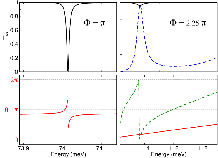
Figure 5: Ground-mode transmission probability (upper panels) and phase (lower panels) around the resonance $\epsilon_{2,1}$ for two different twist angles, namely $\Phi=\pi$ (left panels) and $\Phi=2.25\pi$ (right panels, solid line). In the first case $\epsilon_{2,1}<E_{2}$, and a sharp Fano dip is found. In the second case $\epsilon_{2,1}>E_{2}$, and its position is only indicated by a very shallow dip. In the latter case, also the transmission spectrum of the first-excited mode is reported (dashed line), revealing a pronounced Breit-Wigner resonance.

In fact, as the twist increases from $0$ to $\pi$, both levels $\epsilon_{2,1}$ and $\epsilon_{1,3}$ reach the threshold $E_{1}$. However, while the former shows up as a resonance in the transmission spectrum, the latter disappears as it enters the traveling-states region, with its imaginary part going to zero. Again, this behavior can be traced by the complex scaling method alone, since the lower energy accessible with the QTBM is $E_{1}$. When $\epsilon_{2,1}$ enters the energy range of first-mode traveling states, it appears as a Fano resonance since it is a second-mode quasi-bound state. Moreover, contrary to the other two resonances, it appears with a significant width (bottom panel of Fig. 3) from the beginning, since at $\Phi\simeq 0.85\pi$ the coupling between the modes is already strong.

When the twist increases from $\pi$ to $2\pi$ the three quasi-bound levels described above also increase their energy. However, as $\epsilon_{2,2}$ and $\epsilon_{2,3}$ approach the threshold of the second channel, their width decreases and they finally disappear, with the width going to zero, when their energy reaches $E_{2}$. The behavior of $\epsilon_{2,1}$ is different. In fact, its resonance width is always of the order of $4\mu eV$ until the energy reaches $E_{2}$, where the width increases by order of magnitudes. This is shown in the right panels of Fig. 5, where the transmission probability (top) and phase (bottom) are shown, for a twist $\Phi=2.25\pi$. Here, $\epsilon_{2,1}>E_{2}$, and the second transmission channel becomes available. The solid line is the first-channel to first-channel transmission, and shows a tiny dip at the quasi-bound state position, reminiscent of the prominent Fano dip of the single-channel case. The dashed line is the second-channel to second-channel transmission, showing a clear Breit-Wigner resonance with the corresponding continuous phase lapse of $\pi$. not This is not surprising, since in this case the quasi-bound state has the same transverse mode of the transmission channel.

The case with $\nu=3.95$, with a deeper potential well $V$ in the twisted region, presents additional effects. In fact, at zero twist the energy range between $E_{1}$ and $E_{2}$, where only the ground channel is open, contains bound states of two different transverse modes, namely the first excited ($\epsilon_{2,3}$ and $\epsilon_{2,4}$) and the second excited ($\epsilon_{3,1}$), as shown in Fig. 2. As the wire is twisted, the energy of the above three quasi-bound states increases, as illustrated in the top panel of Fig. 6.

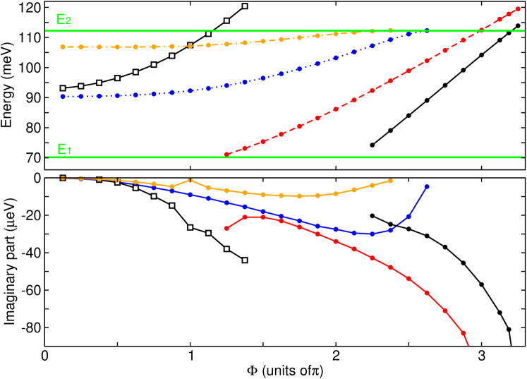
Figure 6: Same as Fig. 3, but for a deeper potential well, with $\nu=3.95$. Here, four quasi-bound states with a first-excited transverse mode are present: $\epsilon_{2,1}$ (solid line, with filled circles), $\epsilon_{2,2}$ (dashed line), $\epsilon_{2,3}$ (dotted line), $\epsilon_{2,4}$ (dot-dashed line), together with a quasi-bound state with a second-excited transverse mode: $\epsilon_{3,1}$ (solid line with empty squares). The two resonances $\epsilon_{3,1}$ and $\epsilon_{2,4}$, with different transverse modes, cross around $\Phi=\pi$ with a repulsion of their imaginary components. All the resonances in the $[E_{1},E_{2}]$ range are of Fano type.

However, the level $\epsilon_{3,1}$ (solid line with empty squares) increases faster than the other two, it crosses $\epsilon_{2,4}$ around $\Phi=\pi$ and goes beyond $E_{2}$. First of all we note again that, in the $[E_{1},E_{2}]$ range, the transport resonances corresponding to the above quasi-bound states are Fano resonances, in agreement with the fact that they originate from a transverse mode different from that of the transport channel. This is shown in the left panels of Fig. 7, reporting the transmission probability and phase of the ground channel at $\Phi=\pi$, just after the crossing. At the crossing, we also find a repulsion of the imaginary component of the eigenvalues, visible in the bottom panel of Fig. 6.

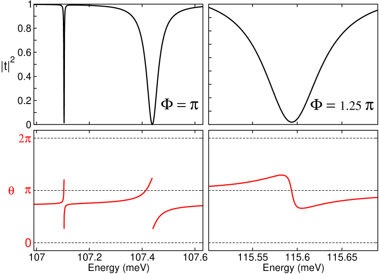
Figure 7: Ground-mode transmission probability (upper panels) and phase (lower panels) showing the resonance $\epsilon_{3,1}$ just after the crossing with $\epsilon_{2,4}$ (at $\Phi=\pi$, left panels) and above the second mode threshold $E_{2}$ (at $\Phi=1.25\pi$, right panels). In the first case the $\pi$ discontinuities of the transmission phase evidence the Fano character of the resonances. In the second case a third channel is available, and the resonance does not present either Fano or Breit-Wigner character.

When $\epsilon_{3,1}>E_{2}$, i.e. it enters the energy region with two transport channels, it does not disappear, as $\epsilon_{2,3}$ and $\epsilon_{2,4}$ do at larger twist, but simply changes its characters. Now the minimum of the dip does not reach zero, and the phase does not present the $\pi$ discontinuity (Fig. 7, right panels). Here in fact, a third transmission channel is available, this lifting the rigid zero-transmission properties of a two-channel case Fano resonance.

As already mentioned, the two resonances $\epsilon_{2,3}$ and $\epsilon_{2,4}$, present in the spectrum since small twist angles, disappear as they reach $E_{2}$, with their width going to zero. Two additional resonances enter the ground-mode region at larger twists: $\epsilon_{2,2}$ and $\epsilon_{2,1}$, represented in Fig. 6 by a dashed line and a solid line, respectively. They are also Fano resonances, but after reaching $E_{2}$ they do not vanish. In fact, their width increases and their minimum does not reach zero, as shown in Fig. 8 for $\epsilon_{2,2}$. Obviously, in this region they are also present in the transmission spectrum of the first-excited channel as Breit-Wigner resonances (dashed line in Fig. 8), since their transverse mode is the first-excited one as well. Correspondingly, their transmission phase presents a smooth evolution of $\pi$.

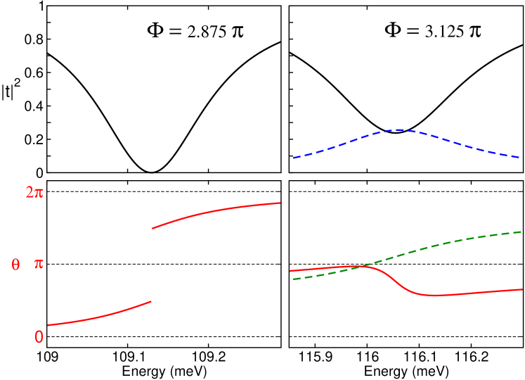
Figure 8: Transmission probability (upper panels) and phase (lower panels) around the resonance $\epsilon_{2,2}$ for the system with $\nu=3.95$. Two different twist angles are considered, with the resonance close to the second-channel threshold: $\Phi=2.875\pi$ (left panels), where $\epsilon_{2,2}<E_{2}$ and $\Phi=3.125\pi$ (right panels), where $\epsilon_{2,2}>E_{2}$. In the second case, both the ground mode (solid line) and first-excited mode (dashed line) transmission probabilities are reported. As for the case of Fig. 7, after the crossing of $E_{2}$ the $\pi$ discontinuity of the phase is lost, due to the availability of a third transmission channel. The broad peak in the first-excited channel is a Breit-Wigner resonance.

V Conclusions

By solving the open-boundary Schrödinger equation through the QTBM we obtained the transmission spectra of the twisted QW. The effect of the twist can be summarized in the following points. First, the twist is able to mix different transmission channels in spite of the fact that the transverse QW section is not altered (but only rotated). Furthermore, bound states of $V$ are coupled to traveling states and appear as resonance peaks/dips in the transmission spectra. No additional resonances are introduced. Second, the character of the resonance depends upon the transverse mode of the original bound state. In fact, when the latter is equal to the transverse mode of the transmission channel, we find a Breit-Wigner resonance, otherwise we find a Fano resonance. In case more than two channels are available, we do not find the $\pi$ discontinuity of the transmission phase typical of Fano resonances. Third, the twist increases the energy of quasi-bound levels. The higher the transverse mode of the quasi-bound state, the faster its energy is increased. However, the change of resonance width is non-monotonic with the twist. In general, it increases from zero when the energy of the bound state is already in the transport region in the straight QW, and decreases as the above energy reaches the threshold of the transmission channel with the same transverse mode as the quasi-bound state. Forth, resonances that are present from the beginning in the first-channel region disappear as they reach $E_{2}$, while resonances that enter the $E_{1}$-$E_{2}$ region at a finite twist, persist in the multi-channel region. The strict behavior described above could help in anticipating the characters of transmission spectra of QW locally twisted once the spectra of the straight wire is known. Furthermore, it supports the idea that the twist can reduce the effects of localized states on quantum conductance, since it shifts their levels towards higher energies, possibly beyond Fermi level of the quasi-1D nanostructure.

APPENDIX: COMPLEX SCALING METHOD

So far we have identified resonant energies with singular points of the reflection/transmission coefficient. In the framework of the complex scaling method, introduced in the ’70 by Aguilar, Baslev and Combes Aguilar and Combes (1971); Balslev and Combes (1971) (for a review see also Ref. Cycon et al., 1987), resonances are identified with the complex eigenvalues of a non-symmetric linear operator obtained from the original one by analytic complex deformation. The real part of such complex-valued eigenvalues coincides with the usual resonance energy level, while the imaginary part is associated with the resonant state lifetime. The complex scaling method has been employed in Ref. Kovařík and Sacchetti, 2007 to twisted QW in order to prove the existence of resonances and here we briefly resume it.

Let $\omega=\left[-\frac{1}{2}L_{y},+\frac{1}{2}L_{y}\right]\times\left[-\frac{1}{2}L_{z},+\frac{1}{2}L_{z}\right]\subset R^{2}$ be the rectangular cross section of our QW. For a given $x\in R$ and $(y,z)\in\omega$ we define the mapping given in Eq. (II) where $\varphi(x)=\epsilon\alpha(x)$ and where $\alpha:R\to R$ is a differentiable function which represent the twisting and ${\epsilon}\geq 0$ is a real-valued parameter which represents the strength of the twisting. Let $\Omega_{{\epsilon}}$ be the twisted QW and let

$${H}_{\epsilon}=-\frac{\hbar^{2}}{2m}\Delta+V(x)$$

be the time independent Schrödinger operator on $\Omega_{{\epsilon}}$, that is the wave function $\psi$ belongs to $L^{2}(\Omega_{{\epsilon}})$ with Dirichlet boundary conditions at $\partial\Omega_{{\epsilon}}$. $V$ represents the external potential Eq. (3), depending only on the longitudinal variable $x$. In the following, for the sake of definiteness, let us assume the units choice such that $\frac{\hbar^{2}}{2m}=1$.

In order to analyze the operator ${H}_{\epsilon}$ we go back to the untwisted tube $\Omega$. The operator $H_{\epsilon}$ then takes the form $K_{\epsilon}$

$$K_{\epsilon}=-\partial_{yy}^{2}-\partial_{zz}^{2}-[\partial_{x}+{\epsilon}\alpha^{\prime}(x)\,\partial_{\tau}]^{2}+V(x)=K_{0}+U_{\epsilon}\,,$$

where

$$\partial_{\tau}=y\partial_{z}-z\partial_{y}$$

and

$$K_{0}=-\partial_{xx}^{2}-\partial_{yy}^{2}-\partial_{zz}^{2}+V(x)$$

and

$$U_{\epsilon} = -[\partial_{x}+{\epsilon}\alpha^{\prime}(x)\,\partial_{\tau}]^{2}+\partial_{xx}^{2}$$

$$= -2{\epsilon}\,\alpha^{\prime}(x)\partial^{2}_{x\tau}-{\epsilon}\,\alpha^{\prime\prime}(x)\,\partial_{\tau}-{\epsilon}^{2}\left[\alpha^{\prime}(x)\right]^{2}\,\partial_{\tau\tau}^{2}\,.$$

The operator $K_{\epsilon}$ is a symmetric operator on $L^{2}(\Omega)$ with Dirichlet boundary conditions at $\partial\Omega$. The spectrum of $K_{0}$ is given by Eq. (5), that is, the spectrum of $K_{0}$ admits embedded eigenvalues in the continuous spectrum. In Ref. Kovařík and Sacchetti, 2007 it has been proved that such embedded eigenvalues become resonances when we add the perturbation $U_{\epsilon}$ to $K_{0}$. Resonances are defined by employing the method of exterior complex scaling to the operator $K_{\epsilon}$, provided that the potential $V$ is a bounded potential which extends to an analytic function with respect to $x$ in some sector, and the twisting function $\alpha(x)$ extends to analytic function with respect to $x$ in a suitable complex set. The exterior complex scaling method consists in introducing the mapping $S_{\theta}$, which acts as a complex dilation in the longitudinal variable $x$:

$$(S_{\theta}\psi)(x,y,z)=e^{\theta/2}\psi(e^{\theta}x,y,z)\,,\quad\theta\in C,\,\Im\theta>0.$$

The transformed operator is not a symmetric operator and it takes the form

$$K_{\epsilon}(\theta)=S_{\theta}K_{\epsilon}S^{-1}_{\theta}=K_{0}(\theta)+U_{\epsilon}(\theta)\,,$$

where

$$K_{0}(\theta)=S_{\theta}K_{0}S^{-1}_{\theta}=-e^{-2\theta}\,\partial_{xx}^{2}-\partial_{yy}^{2}-\partial_{zz}^{2}+V(e^{\theta}x)\,$$

and

$$U_{\epsilon}(\theta) = S_{\theta}U_{{\epsilon}}S^{-1}_{\theta}$$

$$= -2{\epsilon}\,e^{-\theta}\,\alpha^{\prime}(e^{\theta}x)\partial^{2}_{x\tau}-{\epsilon}\,\alpha^{\prime\prime}(e^{\theta}x)\,\partial_{\tau}$$

$$-{\epsilon}^{2}\left[\alpha^{\prime}(e^{\theta}x)\right]^{2}\,\partial_{\tau\tau}^{2}\,.$$

Then, the essential spectrum of $K_{\epsilon}(\theta)$ consists of the sequence of the half-lines (Fig. 9) $E_{n}+e^{-2i\Im\theta}R^{+}$, $n=1,2,\ldots$, and, by a standard argument, it turns out that the eigenvalues of $K_{\epsilon}(\theta)$ are analytic functions of $\theta$, they are in fact independent of $\theta$. These non-real eigenvalues of $K_{\epsilon}(\theta)$, for $\theta$ such that $\Im\theta>0$, are identified with the resonances of $K_{\epsilon}$ (and hence with the resonances of $H_{\epsilon}$) Cycon et al. (1987).

Figure 9: The essential spectrum of $K_{\epsilon}(\theta)$ is given by the half-lines $E_{n}+e^{-2i\Im\theta}R^{+}$ (full lines). The eigenvalues of $K_{\epsilon}(\theta)$ (denoted by open circle) with strictly negative imaginary part are the resonances of $H_{\epsilon}$; for energies below the threshold $E_{1}$ the eigenvalues of $K_{\epsilon}(\theta)$ (denoted by full circle) are purely real valued and they are eigenvalues of $H_{\epsilon}$.

References

- Ihn (2004) T. Ihn, Electronic Quantum Transport in Mesoscopic Semiconductor Structures (Springer, New York, USA, 2004).
- Rurali (2010) R. Rurali, Rev. Mod. Phys. 82, 427 (2010).
- Nöckel and Stone (1994) J. U. Nöckel and A. D. Stone, Phys. Rev. B 50, 17415 (1994).
- Fano (1961) U. Fano, Phys. Rev. 124, 1866 (1961).
- Fransson and Balatsky (2007) J. Fransson and A. V. Balatsky, Phys. Rev. B 75, 153309 (2007).
- Rotter et al. (2004) S. Rotter, F. Libisch, J. Burgdörfer, U. Kuhl, and H.-J. Stöckmann, Phys. Rev. E 69, 046208 (2004).
- Göres et al. (2000) J. Göres, D. Goldhaber-Gordon, S. Heemeyer, M. A. Kastner, H. Shtrikman, D. Mahalu, and U. Meirav, Phys. Rev. B 62, 2188 (2000).
- Miroshnichenko et al. (2010) A. E. Miroshnichenko, S. Flach, and Y. S. Kivshar, Rev. Mod. Phys. 82, 2257 (2010).
- Suzuura (2006) H. Suzuura, Phys. E 34, 674 (2006).
- Tseng et al. (2009) S.-H. Tseng, N.-H. Tai, M.-T. Chang, and L.-J. Chou, Carbon 47, 3472 (2009).
- Kovařík and Sacchetti (2007) H. Kovařík and A. Sacchetti, Journal of Physics A: Mathematical and Theoretical 40, 8371 (2007).
- Breit and Wigner (1936) G. Breit and E. Wigner, Phys. Rev. 49, 519 (1936).
- Fano (1935) U. Fano, Nuovo Cimento 12, 154 (1935).
- Reinhardt (1982) W. P. Reinhardt, Annu. Rev. Phys. Chem. 33, 223 (1982).
- Morse and Feshbach (1953) P. M. Morse and H. Feshbach, Methods of Theoretical Physics, vol II (MacGraw Hill, New York, USA, 1953).
- Lent and Kirkner (1990) C. S. Lent and D. J. Kirkner, J. Appl. Phys. 67, 6353 (1990).
- da Costa (1981) R. C. T. da Costa, Phys. Rev. A 23, 1982 (1981).
- Ferrari and Cuoghi (2008) G. Ferrari and G. Cuoghi, Phys. Rev. Lett. 100, 230403 (2008).
- Cuoghi et al. (2009) G. Cuoghi, G. Ferrari, and A. Bertoni, Phys. Rev. B 79, 073410 (2009).
- Price (1992) P. Price, IEEE Trans. on Electron Devices 39, 520 (1992).
- W. Porod and Lent (1992) Z. S. W. Porod and C. Lent, Appl. Phys. Lett. 61, 1350 (1992).
- (22) Note that in Fig. 5, the abscissa of the right panels has a scale much larger than in the left panels or in Fig. 4. As a consequence, the peaks/dip here reported have a width much larger than the previous case, as described in the text. Also note that the transmission phase has been reduced to the region so that a value of is rescaled and reported as . The vertical dashed line is not a phase jump: on the contrary, it has been introduced to indicate a continuity of the curve, as opposed to the Fano case of the left panel.
- Aguilar and Combes (1971) J. Aguilar and J. M. Combes, Commun. Math. Phys. 22, 269 (1971).
- Balslev and Combes (1971) E. Balslev and J. M. Combes, Commun. Math. Phys. 22, 280 (1971).
- Cycon et al. (1987) H. Cycon, R. G. Froese, W. Kirsch, and B. Simon, Schrödinger Operators: With Application To Quantum Mechanics And Global Geometry (Springer-Verlag, Berlin, 1987).