Static-light meson-meson potentials

Abstract:

We investigate potentials between pairs of static-light mesons in $N_{\mathrm{f}}=2$ Lattice QCD, in different spin channels. The question of attraction and repulsion is particularly interesting with respect to the $X(3872)$ charmonium state and charged candidates such as the $Z^{+}(4430)$. We employ the nonperturbatively improved Sheikholeslami-Wohlert fermion and the Wilson gauge actions at a lattice spacing $a\approx 0.084$ fm and a pseudoscalar mass $m_{\mathrm{P}S}\approx 760$ MeV. We use stochastic all-to-all propagator techniques, improved by a hopping parameter expansion. The analysis is based on the variational method, utilizing various source and sink interpolators.

1 Introduction

We numerically determine ground and excited states of static-light mesons (${\mathcal{B}}=Q\bar{q}$) as well as intermeson potentials between pairs of static-light mesons, ${\mathcal{B}}({\mathbf{r}}){\mathcal{B}}({\mathbf{0}})$ and ${\mathcal{B}}({\mathbf{r}})\overline{\mathcal{B}}({\mathbf{0}})$, with a static quark-quark (or quark-antiquark) separation $r=|{\mathbf{r}}|=Ra$. $a$ denotes the lattice spacing, $Q$ a static colour source and the positions of the light quarks $q$ are not fixed. For large heavy quark masses the spectra of heavy-light mesons are determined by excitations of the light quark and gluonic degrees of freedom. In particular, the vector-pseudoscalar splitting vanishes and the static-light meson ${\mathcal{B}}$ can be interpreted as either a $\overline{B}$, a $\overline{B}^{*}$, a $D$ or a $D^{*}$ heavy-light meson.

Static-light intermeson potentials were first evaluated on the lattice by Michael and Pennanen in the quenched approximation [1] and with $N_{\mathrm{f}}=2$ Sheikholeslami-Wohlert sea quarks [2]. A more detailed quenched study can be found in ref. [3] and the un-quenched case is revisited with twisted mass fermions by Wagner in these proceedings [4]. Meson-antimeson potentials were computed in ref. [2] and, with Wilson sea quarks, in ref. [5]. Graphically, the quark line diagrams that we evaluate can be depicted as,

$$\parbox{13.00806pt}{ \immediate\immediate\ignorespaces \begin{picture}(10.0,40.0)\immediate\ignorespaces\immediate\ignorespaces\immediate\ignorespaces\immediate\ignorespaces\immediate\ignorespaces\put(0.0,0.0){\includegraphics{diag1.1}}\ignorespaces\immediate\ignorespaces \immediate\ignorespaces\immediate\ignorespaces\immediate\ignorespaces\immediate\ignorespaces\immediate\ignorespaces\immediate\ignorespaces\immediate\ignorespaces\immediate\ignorespaces \immediate\ignorespaces{}\end{picture} \immediate\ignorespaces\immediate}\;\;,\;\;\qquad\parbox{34.69038pt}{ \immediate\immediate\ignorespaces \begin{picture}(30.0,40.0)\immediate\ignorespaces\immediate\ignorespaces\immediate\ignorespaces\immediate\ignorespaces\immediate\ignorespaces\put(0.0,0.0){\includegraphics{diag2.1}}\ignorespaces\immediate\ignorespaces \immediate\ignorespaces\immediate\ignorespaces\immediate\ignorespaces\immediate\ignorespaces\immediate\ignorespaces\immediate\ignorespaces\immediate\ignorespaces\immediate\ignorespaces\immediate\ignorespaces\immediate\ignorespaces\immediate\ignorespaces\immediate\ignorespaces\immediate\ignorespaces \immediate\ignorespaces{\put(15.0,-6.0){\makebox(0.0,0.0)[t]{$\leftarrow$ $R$ $\rightarrow$}}}\end{picture} \immediate\ignorespaces\immediate}\;\;,\;\;\;\quad\parbox{34.69038pt}{ \immediate\immediate\ignorespaces \begin{picture}(30.0,40.0)\immediate\ignorespaces\immediate\ignorespaces\immediate\ignorespaces\immediate\ignorespaces\immediate\ignorespaces\put(0.0,0.0){\includegraphics{diag3.1}}\ignorespaces\immediate\ignorespaces \immediate\ignorespaces\immediate\ignorespaces\immediate\ignorespaces\immediate\ignorespaces\immediate\ignorespaces\immediate\ignorespaces\immediate\ignorespaces\immediate\ignorespaces\immediate\ignorespaces\immediate\ignorespaces\immediate\ignorespaces\immediate\ignorespaces\immediate\ignorespaces \immediate\ignorespaces{\put(15.0,-6.0){\makebox(0.0,0.0)[t]{$\leftarrow$ $R$ $\rightarrow$}}}\end{picture} \immediate\ignorespaces\immediate}\;\;,$$ (1)

where the static-light correlation function is shown on the left, and those for the meson-meson and meson-antimeson cases in the centre and on the right, respectively. Straight lines represent static quark propagators and wiggly lines light quark propagators. In this paper we neglect explicit meson exchange (i.e. “box” and “cross”) diagrams. The analyses of these as well as of a larger lattice volume are in progress. This means that here we only consider the isospin $I=0$ ${\mathcal{B}}{\mathcal{B}}$ and the $I=1$ ${\mathcal{B}}\overline{\mathcal{B}}$ combinations.

The static-light correlation function in Euclidean time $t=Ta$ is given by,

$$C(t)=\langle 0|(\overline{Q}_{\alpha}\;\mathcal{O}_{\alpha\beta}\;q_{\beta})_{x+t\hat{4}}\;(\bar{q}_{\gamma}\;\mathcal{O}_{\gamma\delta}\;Q_{\delta})_{x}|0\rangle=\left\langle\;\mathrm{Tr}\;\left[\prod^{T-1}_{k=0}\,U^{\dagger}_{x+ka\hat{4},4}\;\frac{\Eins+\gamma_{4}}{2}\;\mathcal{O}\;M^{-1}_{x+t\hat{4},x}\;\mathcal{O}\right]\right\rangle_{\!\!\!U}\;.$$ (2)

The trace is over colour (not displayed) and Dirac indices, $\left\langle\cdot\right\rangle_{U}$ indicates the expectation value over gauge configurations and $\hat{\mu}$ denotes a unit vector in $\mu$-direction. We average over all possible source points $x/a\in\{1,\ldots,L_{\sigma}\}^{3}\times\{1,\ldots,L_{\tau}\}$ to reduce statistical errors where $x=({\mathbf{x}},x_{4})$. The correlator is automatically zero-momentum projected since ${\mathbf{x}}$ is the same at source and sink, due to the static propagator. $M^{-1}_{yx}=\langle q_{y}\bar{q}_{x}\rangle$ is the propagator for the light quark $q$ on a given gauge configuration and $U_{x,\mu}$ is the gauge link connecting the lattice site $x$ with $x+a\hat{\mu}$. The absence of the spin in the static propagator necessitates the $(\Eins+\gamma_{4})/2$ Dirac projection of the (fermionic) static-light “meson” to fix the parity $P$. This is very similar to baryonic correlation functions where a spin $\frac{1}{2}$ source is created by three (rather than one) light quarks. Meson-(anti)meson correlation functions can be obtained by combining the above correlator with another one that is spatially shifted by a distance ${\mathbf{r}}$, before taking the gauge average.

2 Representations and classification of states

In the continuum limit, the static-light states can be classified according to fermionic representations $J^{P}$ of the rotation group ${\mathrm{O}(3)}$. At vanishing distance ${\mathbf{r}}={\mathbf{0}}$ the ${\mathcal{B}}{\mathcal{B}}$ and ${\mathcal{B}}\overline{\mathcal{B}}$ states can be characterized by integer $J^{P}$ and $J^{PC}$ quantum numbers, respectively. However at $r=|{\mathbf{r}}|>0$ the $\mathrm{O(3)}$ (or $\mathrm{O(3)}\otimes{\mathcal{C}}$) symmetry is broken down to its cylindrical $\mathrm{D_{\infty h}}$ subgroup. The irreducible representations of this are conventionally labelled by the spin along the axis $\Lambda$, where $\Sigma,\Pi,\Delta$ refer to $\Lambda=0,1,2$, respectively, with a subscript $\eta=g$ for gerade (even) $PC=+$ or $\eta=u$ for ungerade (odd) $PC=-$ transformation properties with respect to the midpoint. All $\Lambda\geq 1$ representations are two-dimensional. The one-dimensional $\Sigma$ representations carry an additional $\sigma_{v}=\pm$ superscript for their reflection symmetry with respect to a plane that includes the two endpoints.

To create states of different $J^{P(C)}$ we use operators $\mathcal{O}$ that contain combinations of Dirac $\gamma$-matrices and covariant lattice derivatives $\nabla[U]$ that act on a fermion spinor $q$ as,

$$\nabla_{\mu}q_{x}=U_{x,\mu}q_{y+a\hat{\mu}}-U_{x,-\mu}q_{x-a\hat{\mu}}\,,\quad\mbox{where}\quad U_{x,-\mu}=U^{\dagger}_{y-a\hat{\mu},\mu}\,.$$ (3)

On the lattice the continuum rotational symmetry is broken and the groups $\mathrm{O(3)}$ and $\mathrm{D_{\infty h}}$ need to be replaced by their finite dimensional subgroups $\mathrm{O_{h}}$ and $\mathrm{D_{4h}}$, respectively. We label fermionic representations of the octahedral group $\mathrm{O_{h}}$ as $\mathrm{O_{h}}^{\prime}$. For fermionic representations of $\mathrm{D_{\infty h}}$ that we do not need in the present context, see ref. [6]. It is well known, see e.g. ref. [7], that the assignment of a continuum spin to a lattice result can be ambiguous, in particular for radial excitations because a given $\mathrm{O_{h}}$ representation can be subduced from several continuum $J$s. For instance,

$$G_{1}\leftarrow J=\frac{1}{2},\frac{7}{2},\dots\,,\quad H\leftarrow J=\frac{3}{2},\frac{5}{2},\dots\,,\quad A_{1}\leftarrow J=0,4,\dots\,,\quad T_{1}\leftarrow J=1,3,4,\dots\,.$$ (4)

For $\Lambda\leq 2$ the mapping of continuum $\mathrm{D_{\infty h}}$ onto discrete $\mathrm{D_{4h}}$ representations is more straight forward. Hence in this case we adopt the continuum notation only.

The operators that we used to create the static-light mesons are displayed in table 1 (see, e.g., ref. [8]).

$\mathcal{O}$	wave [8]	$\mathrm{O_{h}}^{\prime}$ rep.	continuum $J^{P}$	$J^{P}$ (heavy-light)
$\gamma_{5}$	$S$	$G_{1}^{+}$	$\frac{1}{2}^{+}$	$0^{-},1^{-}$
$\Eins$	$P_{-}$	$G_{1}^{-}$	$\frac{1}{2}^{-}$	$0^{+},1^{+}$
$\gamma_{i}\nabla_{i}$	$P_{-}$	$G_{1}^{-}$	$\frac{1}{2}^{-}$	$0^{+},1^{+}$
$\left(\gamma_{1}\nabla_{1}-\gamma_{2}\nabla_{2}\right)+\mathrm{cycl.}$	$P_{+}$	$H^{-}$	$\frac{3}{2}^{-}$	$1^{+},2^{+}$

Table 1: Operators and representations for static-light mesons. In the last column we display the $J^{P}$ for a heavy-light meson, obtained by substituting the (spinless) static source by a heavy fermion.

$\mathcal{O}\;\otimes\;\mathcal{O}$	${\mathcal{B}}{\mathcal{B}}$		${\mathcal{B}}\overline{\mathcal{B}}$
	$r=0$: $J^{P}$	$r>0$: $\Lambda_{\eta}^{(\sigma_{\nu})}$	$r=0$: $J^{PC}$	$r>0$: $\Lambda_{\eta}^{(\sigma_{\nu})}$
$\gamma_{5}\;\otimes\;\gamma_{5}$	$0^{+},1^{+}$	$\Sigma_{g}^{+},\Pi_{g}$	$0^{++},1^{+-}$	$\Sigma_{g}^{+},\Sigma_{u}^{-},\Pi_{u}$
$\Eins\;\otimes\;\Eins$	$0^{+},1^{+}$	$\Sigma_{g}^{+},\Pi_{g}$	$0^{++},1^{+-}$	$\Sigma_{g}^{+},\Sigma_{u}^{-},\Pi_{u}$
$\gamma_{5}\;\otimes\;\Eins$	$0^{-},1^{-}$	$\Sigma_{u}^{-},\Pi_{u}$	$0^{-+},1^{--}$	$\Sigma_{u}^{-},\Sigma_{g}^{+},\Pi_{g}$
$\gamma_{5}\;\otimes\;\gamma_{i}\nabla_{i}$	$0^{-},1^{-}$	$\Sigma_{u}^{-},\Pi_{u}$	$0^{-+},1^{--}$	$\Sigma_{u}^{-},\Sigma_{g}^{+},\Pi_{g}$
$\gamma_{5}\;\otimes\;[\left(\gamma_{1}\nabla_{1}-\gamma_{2}\nabla_{2}\right)\;+\mathrm{cycl.}]$	$1^{-},2^{-}$	$\Sigma_{u}^{+},\Pi_{u},\Delta_{u}$	$1^{--},2^{-+}$	$\Sigma_{g}^{+},\Pi_{g},\Sigma_{u}^{+},\Pi_{u},\Delta_{u}$
$\gamma_{i}\nabla_{i}\;\otimes\;[\left(\gamma_{1}\nabla_{1}-\gamma_{2}\nabla_{2}\right)\;+\mathrm{cycl.}]$	$1^{+},2^{+}$	$\Sigma_{g}^{-},\Pi_{g},\Delta_{g}$	$1^{+-},2^{++}$	$\Sigma_{u}^{-},\Pi_{u},\Sigma_{g}^{+},\Pi_{g},\Delta_{g}$

Table 2: Operators and continuum representations for the meson-meson (${\mathcal{B}}{\mathcal{B}}$) and meson-antimeson (${\mathcal{B}}\overline{\mathcal{B}}$) potentials.

The intermeson potentials were obtained by combining two static-light mesons of different (or the same) quantum numbers. This can be projected into an irreducible $\mathrm{D_{\infty h}}$ representation, either by coupling the light quarks together in spinor space [4] or by projecting the static-light meson spins into the direction $\hat{\mathbf{r}}$ of the static source distance, by applying $\frac{1}{2}(\Eins\pm i\gamma_{5}\boldsymbol{\gamma}\cdot\hat{\mathbf{r}})$, and taking appropriate symmetric ($\Lambda_{s}=1$) or antisymmetric ($\Lambda_{s}=0$) spin combinations. These two approaches can be related to each other via a Fierz transformation. For the preliminary results presented here we have not yet performed this projection and different representations will mix. The analyzed operators and the corresponding representations are listed in table 2.

For $J>0$ and $r>0$ the irreducible representations of $\mathrm{O(3)}$ split up into two or more irreducible representations of $\mathrm{D_{\infty h}}$. For instance the angular momentum of the $P_{+}$ operator within our $1^{-},2^{-}$ $r=0$ state can be perpendicular or parallel to the intermeson axis. For the axis pointing into the $\hat{3}$-direction, we call the $S\otimes P_{+}$ operator $\gamma_{5}\otimes(\gamma_{1}\nabla_{1}-\gamma_{2}\nabla_{2})$ “parallel” ($\|$) and the other combinations “perpendicular” ($\bot$). The $\bot$ state has no angular momentum pointing into the direction of the axis and hence only couples with the light quarks to $\Sigma_{u}^{+}$ and $\Pi_{u}$. Vice versa, the $\|$ operator can only create $\Pi_{u}$ and $\Delta_{u}$ states but not the $\Sigma_{u}^{+}$.

3 Simulation and analysis

volume $L_{\sigma}^{3}\times L_{\tau}$	$\beta$	$\kappa_{\mathrm{val}}=\kappa_{\mathrm{sea}}$	$c_{\mathrm{SW}}$	$a/\mathrm{fm}$	$La/\mathrm{fm}$	$m_{\mathrm{PS}}/\mathrm{MeV}]$	$N_{\mathrm{conf}}$
$16^{3}\times 32$	$5.29$	$0.13550$	$1.9192$	$0.084$	$1.34$	$760(3)$	$200$

Table 3: Lattice parameters.

We employ $N_{\mathrm{f}}=2$ Sheikholeslami-Wohlert configurations generated by the QCDSF Collaboration [9]. The parameter values are listed in table 3, where the scale is set using $r_{0}(\beta,\kappa)=0.467$ fm. The pseudoscalar mass corresponds to its infinite volume value. We use the Chroma software system [10].

To achieve high statistics in the evaluation of the diagrams eq. (1), all-to-all propagators need to be computed. This is done using stochastic estimator techniques, see ref. [11] and references therein. We generate 300 complex ${\mathbb{Z}}_{2}$ noise sources and apply the hopping parameter expansion to reduce the stochastic variance [12, 5, 11]. Furthermore we enhance the signal over noise ratio by employing a static action with reduced self-energy [5]. This is done by applying one stout smearing step [13] with the parameter $\rho=1/6$ to the temporal links, used to calculate the static propagators. Wuppertal smearing [14] is applied to the source and sink operators, where we employ spatially smeared parallel transporters [5] with the parameters $n_{\mathrm{iter}}=15$, $\alpha=2.5$. The Wuppertal smearing hopping parameter value $\kappa_{\mathrm{w}}=0.3$ is combined with three iteration numbers $N_{\mathrm{iter}}\in\{16,50,100\}$. Masses are then extracted from the resulting correlation matrices, by means of the variational method [15], solving a generalized eigenvalue problem. Errors are calculated using the jackknife method.

4 Results

The eigenvalues $\lambda^{(k)}(t,t_{0})$ of the generalized eigenvalue problem [15],

$$C_{ij}(t)u_{j}^{(k)}=\lambda^{(k)}(t,t_{0})C_{ij}(t_{0})u_{j}^{(k)}\,,$$

are fitted to one- and two-exponential ansätze, to obtain the $k$th mass. The appropriate values of $t_{0}$ and the fit ranges in $t$ are determined from monitoring the effective masses,

$$m_{\mathrm{eff},t_{0}}^{(k)}(t+a/2)=a^{-1}\ln\left(\frac{\lambda^{(k)}(t,t_{0})}{\lambda^{(k)}(t+a,t_{0})}\right)\,.$$

On the left hand side of figure 1, we display the effective ground state energy levels $E_{\mathrm{eff}}$ for $t_{0}=2a$ of the $\gamma_{5}\otimes\gamma_{5}$ ${\mathcal{B}}{\mathcal{B}}$ system for different distances $R=r/a$. In the limit $r\rightarrow\infty$ these will approach the sum of two $\frac{1}{2}^{+}$ static-light meson effective masses (dotted curve). At short distances we see attraction in this channel. The quality of the effective mass plateaus deteriorates with decreasing distance since the wavefunction of such interacting states becomes more than the mere product of our two static-light meson interpolators. We should also keep in mind that so far we did not perform the singlet spin projection and hence there will be additional pollution from the $\Pi_{g}$ state, see table 2. For the example displayed, we perform two-exponential fits to the $t/a\in\{4,\ldots,10\}$ data to obtain the masses.

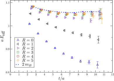
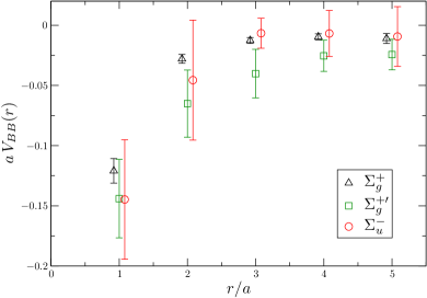
Figure 1: Effective groundstate masses of the $\gamma_{5}\otimes\gamma_{5}$ operator at different distances (left hand side). The dotted line corresponds to twice this mass for a single $\frac{1}{2}^{+}$ static-light meson. The intermeson potential $V(r)$ for the combinations $\gamma_{5}\otimes\gamma_{5}$ ($\Sigma_{g}^{+},\Sigma_{g}^{+\prime}$) and $\gamma_{5}\otimes 1$ ($\Sigma_{u}^{-}$) (right hand side).

We define intermeson potentials as the difference between the meson-meson energy levels and the $r\rightarrow\infty$ two static-light meson limiting cases:

$$V_{\!\mathcal{B}_{1}\mathcal{B}_{2}}(r)=E_{\!\mathcal{B}_{1}\mathcal{B}_{2}}(r)-\left(m_{\!\mathcal{B}_{1}}+m_{\!\mathcal{B}_{2}}\right)\quad\stackrel{{\scriptstyle r\rightarrow\infty}}{{\longrightarrow}}\quad 0\,.$$ (5)

The results for the groundstate ($\Sigma_{g}^{+}$) and the first excited state ($\Sigma_{g}^{+\prime}$) of the $\gamma_{5}\otimes\gamma_{5}$ operator and the $\Sigma_{u}^{-}$ groundstate of $\gamma_{5}\otimes\Eins$ are plotted on the right hand side of figure 1. In all these $I=0$ channels there is attraction of the order of 50 MeV at a distance of $0.2$ fm.

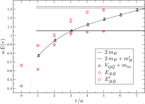
Figure 2: Effective masses for the $\gamma_{5}\otimes\gamma_{5}$ $\mathcal{B}\overline{\mathcal{B}}$ ground and first excited states (red symbols). The horizontal lines denote sums of two static-light meson masses while the black curve and symbols are the static $Q\overline{Q}$ potential, offset by the scalar $a_{0}$ meson mass.

In figure 2 we display the ground state and first excited state energy levels for the ${\mathcal{B}}\overline{\mathcal{B}}$ meson-antimeson case in the $\gamma_{5}\otimes\gamma_{5}$ channel. The two horizontal lines correspond to twice the ground state mass of the $\frac{1}{2}^{+}$ static-light meson and to the sum of its ground and its first excited state masses, the expected $r\rightarrow\infty$ limits. At first sight there appear to be very substantial short distance attractive forces in this channel. However, states consisting of a $Q\overline{Q}$ static potential and a scalar $I=1$ particle will have the same quantum numbers. For our lattice parameters the $a_{0}$ meson is the lowest such state, with masses of two pseudoscalars as well as of a $P$-wave vector lying higher. We include the sum of these two masses in the figure. The ground state ${\mathcal{B}}\overline{\mathcal{B}}$ energy still lies below this level but to decide whether we effectively see the sum of $a_{0}$ and the static potential and to disentangle which $I=1$ $\Sigma_{g}^{+}$ energy level is the lowest one, interactions of the $a_{0}$ with the static potential will have to be taken into account. We hope that simulations on a larger volume will help to clarify this.

5 Conclusions

We investigated interactions between pairs of static-light mesons and found attraction in the $I=S=0$ sector. Meson-antimeson potentials are also very interesting with respect to charmonium threshold states [16] ($D\overline{D}$ molecules or tetraquarks) but difficult to disentangle from mesons that are bound to static-static states (hadro-quarkonium [17]). We are in the process to extend our study to $I=1$ ${\mathcal{B}}{\mathcal{B}}$ and to $I=0$ ${\mathcal{B}}\overline{\mathcal{B}}$ states and to disentangle $S_{\hat{\mathbf{r}}}=\pm 1$ from $S_{\hat{\mathbf{r}}}=0$ states. Also simulations on a larger volume are in progress.

- [1] C. Michael and P. Pennanen [UKQCD Collaboration], Two heavy-light mesons on a lattice, Phys. Rev. D 60 (1999) 054012 [arXiv:hep-lat/9901007].
- [2] P. Pennanen, C. Michael and A. M. Green [UKQCD Collaboration], Interactions of heavy-light mesons, Nucl. Phys. Proc. Suppl. 83 (2000) 200 [arXiv:hep-lat/9908032].
- [3] W. Detmold, K. Orginos and M. J. Savage, potentials in quenched lattice QCD, Phys. Rev. D 76 (2007) 114503 [arXiv:hep-lat/0703009].
- [4] M. Wagner [ETM Collaboration], Forces between static-light mesons, arXiv:1008.1538 [hep-lat].
- [5] G. S. Bali, H. Neff, T. Düssel, T. Lippert and K. Schilling, Observation of string breaking in QCD, Phys. Rev. D 71 (2005) 114513 [arXiv:hep-lat/0505012].
- [6] J. Najjar and G. Bali, Static-static-light baryonic potentials, PoS LAT2009 089 [arXiv:0910.2824 [hep-lat]].
- [7] G. S. Bali, QCD forces and heavy quark bound states, Phys. Rept. 343 (2001) 1 [arXiv:hep-ph/0001312].
- [8] C. Michael and J. Peisa, Maximal variance reduction for stochastic propagators with applications to the static quark spectrum, Phys. Rev. D 58 (1998) 034506 [arXiv:hep-lat/9802015].
- [9] A. Ali Khan et al. [QCDSF Collaboration], Accelerating the hybrid Monte Carlo algorithm, Phys. Lett. B 564 (2003) 235 [arXiv:hep-lat/0303026].
- [10] R. G. Edwards and B. Joó, The Chroma software system for Lattice QCD, Nucl. Phys. Proc. Suppl. 140 (2005) 832 [hep-lat/0409003]; C. McClendon, Optimized Lattice QCD kernels for a Pentium 4 cluster, Jlab preprint (2001) JLAB-THY-01-29 , http://www.jlab.org/~edwards/qcdapi/reports/dslash_p4.pdf.
- [11] G. S. Bali, S. Collins and A. Schäfer, Effective noise reduction techniques for disconnected loops in Lattice QCD, Comput. Phys. Commun. 181 (2010) 1570 [arXiv:0910.3970 [hep-lat]].
- [12] C. Thron, S. J. Dong, K. F. Liu and H. P. Ying, Padé- estimator of determinants, Phys. Rev. D 57 (1998) 1642 [arXiv:hep-lat/9707001].
- [13] C. Morningstar and M. J. Peardon, Analytic smearing of SU(3) link variables in Lattice QCD, Phys. Rev. D 69 (2004) 054501 [hep-lat/0311018].
- [14] S. Güsken et al., Non-singlet axial vector couplings of the baryon octet in lattice QCD, Phys. Lett. B 227 (1989) 266.
- [15] C. Michael, Adjoint sources in Lattice Gauge Theory, Nucl. Phys. B 259 (1985) 58.
- [16] N. Brambilla et al., Heavy quarkonium: progress, puzzles, and opportunities, arXiv:1010.5827 [hep-ph].
- [17] S. Dubynskiy and M. B. Voloshin, Hadro-charmonium, Phys. Lett. B 666 (2008) 344 [arXiv:0803.2224 [hep-ph]].